The simulation of molecular clouds formation in the Milky Way
Abstract
Using 3D hydrodynamic calculations we simulate formation of molecular clouds in the Galaxy. The simulations take into account molecular hydrogen chemical kinetics, cooling and heating processes. Comprehensive gravitational potential accounts for contributions from the stellar bulge, two and four armed spiral structure, stellar disk, dark halo and takes into account self-gravitation of the gaseous component. Gas clouds in our model form in the spiral arms due to shear and wiggle instabilities and turn into molecular clouds after Myr. At the times Myr the clouds form hierarchical structures and agglomerations with the sizes of pc and greater. We analyze physical properties of the simulated clouds and find that synthetic statistical distributions like mass spectrum, ”mass-size” relation and velocity dispersion are close to those observed in the Galaxy. The synthetic (galactic longitude - radial velocity) diagram of the simulated molecular gas distribution resembles observed one and displays a structure with appearance similar to Molecular Ring of the Galaxy. Existence of this structure in our modelling can be explained by superposition of emission from the galactic bar and the spiral arms at 3-4 kpc.
keywords:
galaxies: ISM — Galaxy: structure — ISM: clouds1 Introduction
Molecular clouds represent one of the major constituents of our galaxy (Dame et al. , 2001). Their masses and sizes vary in a wide range (e.g. Solomon et al. , 1987). Molecular clouds play very important role in determination of the structure and evolution of the Galaxy. This can be illustrated by the fact that the stars and their clusters originate from molecular clouds (Shu et al. , 1987; McKee & Ostriker, 2007; Lada & Lada, 2003). The dynamical time of disintegration for molecular clouds in the Milky Way is much shorter than the rotation period of the galaxy (e.g. Blitz & Shu, 1980). So, explanation of the observational fact of existence of the rich population of molecular clouds requires involvement of efficient mechanisms leading to formation of molecular clouds in the Galaxy. Special interest is paid to formation of the giant molecular clouds (GMC) which have masses (Dame et al. , 1986). Two main theories of the GMC formation were proposed. The first one explains formation of the GMCs by large scale magnetic and/or gravitational instabilities (Elmegreen, 1979; Balbus & Cowie, 1985; Elmegreen, 1994; Chou et al. , 2000; Kim & Ostriker, 2006). In the second one the GMCs are built up by coalescence of the smaller molecular clouds (Field & Saslaw, 1965; Levinson & Roberts, 1981; Tomisaka, 1984; Roberts & Stewart, 1987; Kwan & Valdes, 1987) or interaction of the turbulent flows (e.g. Ballesteros-Paredes et al. , 2007). In reality both types of processes are expected to play significant role (Zhang & Song, 1999; Dobbs, 2008).
Large scale perturbations in a gas of the Galactic disk can be generated not only by magnetic fields or self-gravity, but also by the galactic spiral shock wave (Roberts, 1969; Nelson & Matsuda, 1977). A simple analysis of the global galactic shock wave shows that such shocks are unstable (Mishurov & Suchkov, 1975). Obviously, large scale shear flows in the Galactic shocks lead to the development of both wiggle and Kelvin-Helmholz instabilities (Wada, 2001; Wada & Koda, 2004). Such hydrodynamic instabilities are expected to give a birth to spurs, gaseous fragments and turbulent flows (Wada, 1994; Wada et al. , 2000; Dobbs & Bonnel, 2006; Shetty & Ostriker, 2006). The gravitational and thermal (in general, thermo-chemical) instabilities are expected to develop further fragmentation, which leads to formation of the population of molecular clouds.
The properties of molecular clouds (mass, size, density, temperature etc.) are intensively studied both observationally (Solomon et al. , 1987; Falgarone et al. , 1992; Lada et al. , 2008; Heyer et al. , 2009; Rathborne et al. , 2009; Kauffmann et al. , 2010; Román-Zúñiga et al. , 2010) and numerically (Dobbs et al. , 2006; Dobbs & Bonnell, 2007a, b; Tasker & Tan, 2009; Glover & Mac Low, 2011). Efforts in order to understand dependencies between physical parameters of the clouds lead to establishment of several empirical relationships for the properties of molecular clouds (Larson, 1981). In particular, the mass-size relation reflects the hierarchical spatial structure of clouds (Beaumont et al. , 2012). Molecular clouds can agglomerate in small groups and chains, thus reflecting processes of the cloud formation: disintegration into smaller clumps or combining into bigger clouds. Due to the origin of the clouds from the large scale perturbations in the galactic disk molecular clouds can trace the large-scale structures, e.g. spiral arms and the bar (e.g. Wada & Koda, 2004). Several observational studies display existence of the galactic molecular ring (Stecker et al. , 1975; Cohen & Thaddeus, 1977; Roman-Duval et al. , 2010), however it is unclear whether this is an actual ring or just superposition of emission from molecular clouds belonging to different spiral arms (Dobbs & Burkert, 2012).
In this paper we develop a model aiming to reproduce general characteristics of the formation of molecular clouds in the Galaxy, their physical properties, their distribution in the Milky Way using the 3D simulations with the comprehensive gravitational potential, self-gravity of gaseous component, molecular hydrogen chemical kinetics, cooling and heating processes.
The paper is organized as follows. Section 2 describes basic premises and equations of our model. Section 3 presents numerical results on the disk evolution. Section 4 presents analysis of the physical properties of the clouds in our model. Section 5 considers large-scale structures in the simulated Galaxy. Section 6 summarizes the results.
2 Model
2.1 Gas dynamics and galaxy potential
The dynamics of the chemically reacting gas mixture in our model of the Galaxy can be written in the single-fluid approximation as follows:
| (1) |
| (2) |
| (3) |
| (4) |
where is the gas density, is the gas pressure, is the gas velocity vector, is the number of components in the gas mixture (in our model ), is the mass fraction of i-th component of gas, , is the formation/destruction rate of i-th component, is the total energy, is the specific internal energy, and are the cooling and heating rates, correspondingly, is the gravitational potential of gas, is the total external gravitational potential produced by the massive dark halo , the stellar bulge and the stellar disk . The latter includes the potentials of the spiral structure and the bar. The potential of the gaseous component is determined by the Poisson equation:
| (5) |
Hereafter we assume . The external gravitational potential can be written as follows:
| (6) |
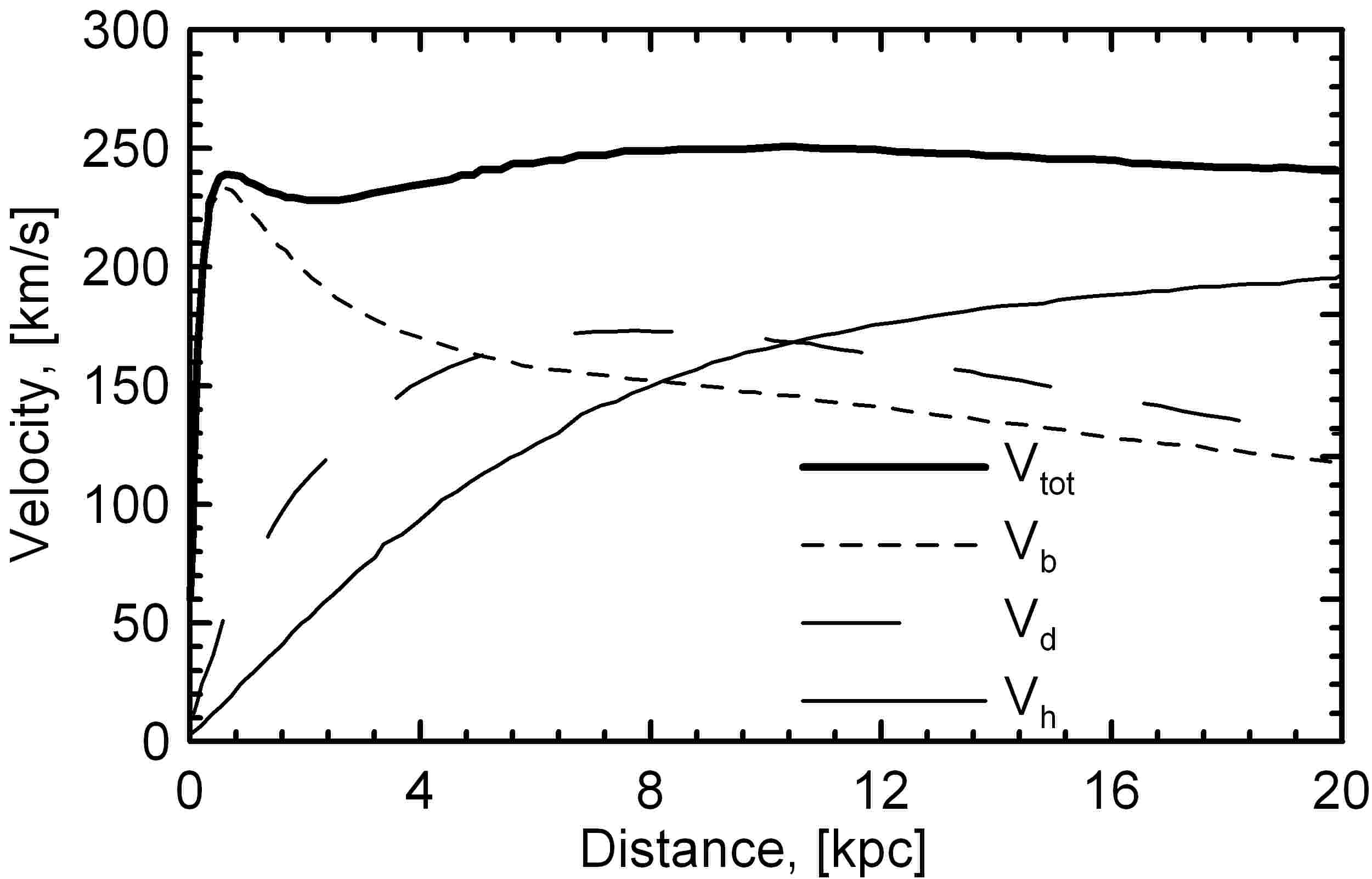
Figure 1 present the rotation curve of the gas components adopted in our model of the Galaxy. For the maximum rotation velocity of the Milky Way we adopt a value obtained from the analysis of the recent observational data on the Galactic masers (Bobylev & Bajkova, 2010). The external gravitational potential of the Galactic subsystems, e.g. stellar bulge, stellar disk and dark halo, , produces this rotation curve with the parameters for the Galactic subsystems fitted by Khoperskov & Tiurina (2003). The detailed description of the gravitational potential components is given in Appendix.
In our calculations we use the value of the angular velocity km s-1 pc-2 as a fiducial value. This value is realized at the radius of corotation kpc (Bobylev & Bajkova, 2010). Our simulations have shown that variation of in the range km s-1 pc-2 (Amores et al. , 2009; Sofue et al. , 2009; Lepine et al. , 2001) does not produce significant changes in the general properties of evolution of gas in the simulated Galaxy.
2.2 Chemical kinetics
H2 molecules in the interstellar medium are formed on the surface of the dust grains and dissociated by ultraviolet Lyman-Werner photons and cosmic rays. We suppose that the dust density is proportional to the gas density because the dust is well mixed with gas on the scales of our simulations. Thus, evolution of molecular hydrogen number density can be found from (Bergin et al. , 2004)
| (7) |
where , are the number densities of atomic and molecular hydrogen, correspondingly, is the total number density of hydrogen species, is the H2 column density, is the H2 formation rate on dust grains (Tielens & Hollenbach, 1985), is the efficiency of the H2 formation on dust (Cazaux & Tielens, 2004), s-1 is the cosmic ray ionization rate, is the extinction. Following Draine & Bertoldi (1996) the photodissociation rate can be estimated as:
| (8) |
where sec-1 is the unshielded photodissociation rate, is the H2 self-shielding factor, is the dust absorption factor.
To calculate the factors and we need to know both molecular, , and total, , hydrogen column densities. In order to do this accurately we should find a cumulative ultraviolet radiation field produced by the young stars and their clusters. Obviously, this problem is extremely complex, moreover, star formation processes are not included in our model. Hence, we follow a simplified approach introduced by Dobbs (2008). We use a simple estimate that the column densities of the chemical species are just the local densities of these species multiplied by the typical distance to a young star, : . This distance is assumed to be a constant length scale for the whole disk. In our simulations we take pc, which is in agreement with the number of massive stars expected from the Salpeter initial mass function.
We assume that the Galactic gas has solar metallicity with the abundances given in Asplund et al. (2005): . We assume that the dust depletion factors are equal to 0.72, 046 and 0.2 for C, O and Si, correspondingly. Chemical kinetics of the heavy elements is not solved in our model the. We suppose that the carbon and silicon are singly ionized and oxygen stays neutral. This assumption is acceptable for the interstellar medium of the Milky Way due to existence of the strong ultraviolet radiation in the range 10-13 eV (Habing, 1968).
2.3 Cooling and heating processes
The cooling rates are computed separately for the temperatures below and above K. In the low temperature range the cooling rate in the energy equation (4) includes the typical processes of radiative losses for the interstellar medium: cooling due to recombination and collisional excitation and free-free emission of hydrogen (Cen, 1992), molecular hydrogen cooling (Galli & Palla, 1998), cooling in the fine structure and metastable transitions of carbon, oxygen and silicon (Hollenbach & McKee, 1989), energy transfer in collisions with the dust particles (Wolfire et al. , 2003) and recombination cooling on the dust (Bakes & Tielens, 1994). In the high temperature range, K, the cooling rate for solar metallicity is taken from Sutherland & Dopita (1993). We note that in our calculations the gas temperature is generally below K, higher temperature is reached only in small rarefied regions at the periphery of the disk.
The heating rate in the equation (4) takes into account photoelectric heating on the dust particles (Bakes & Tielens, 1994; Wolfire et al. , 2003), heating due to H2 formation on the dust, and the H2 photodissociation (Hollenbach & McKee, 1979) and the ionization heating by cosmic rays (Goldsmith et al. , 1978).
2.4 Numerical methods
To solve the system of gas dynamical equations (1-4) we use nonlinear finite-volume numerical scheme TVD MUSCL in the Cartesian coordinates (van Leer, 1979). The continuity equation for chemical species is constructed using the operator splitting scheme. Note that because in our model we have two chemical species, HI and H2, we can solve the kinetics equation for one of them only, e.g. for H2. At first we solve the continuity equation without right-hand terms and update the H2 density due to advection. Than we update this result after solution of chemical reactions. The equation for H2 (7) is integrated using a fourth-order Runge-Kutta method. To find the gravitational potential of the gas (5) we use the TreeCode method (Barnes & Hut, 1986).
The numerical resolution is cells. The cells are assumed to be cubic with the sides of 7.3 pc. Therefore, the physical size of the computational grid is kpc. We also made calculations with higher resolution in the vertical direction, but lower in the disk plane direction, e.g. , and did not find significant difference in global characteristics of gas evolution. We expect that this is sufficient to model the large scale dynamics of the Galactic disk and to study the formation of the spurs and molecular clouds in the vicinity of the spiral arms.
3 Disk evolution
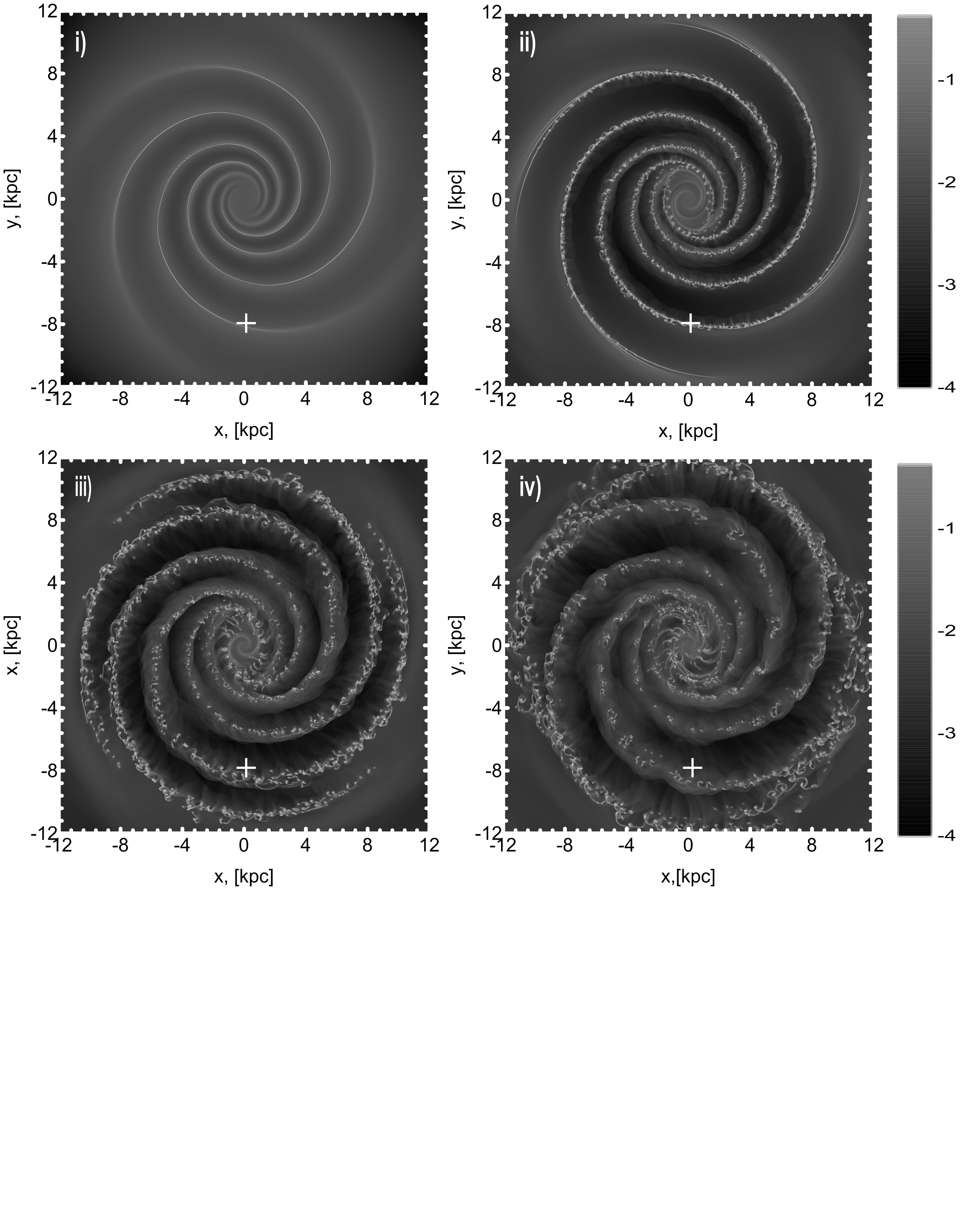
Figure 2 shows the surface gas density at 50, 100, 200 and 300 Myr. At the beginning the spiral shocks are formed due to the supersonic gas flow through the spiral gravitational potential of the stellar disk. After Myr one finds a well-developed spiral structure in the gas disk (upper left panel). The width of the gas spirals is significantly smaller than that of the stellar density wave due to higher stellar velocity dispersion. Owing to shear and wiggle instabilities the shock front becomes perturbed, and as a result the spurs and fragments are formed. Such spurs and fragments can be found at Myr (upper left panel) and are clearly seen at Myr (upper right panel). On one hand, higher density in such fragments stimulates molecular hydrogen formation and, as a consequence, efficient cooling of gas in the fragments. On the other hand, the cooling can lead to further fragmentation. We find that the efficient molecule formation starts at Myr, which corresponds to the time scale of molecular hydrogen formation on the dust grains. A major part of the H2 molecules is formed in such fragments, which are the progenitors of molecular clouds. Note that a number of fragments formed may have super-Jeans masses. So, further fragmentation is expected to be amplified by both thermal instability and self-gravity.
A large number of clouds is formed as a result of further evolution: a flocculent structure in the spiral arms can be clearly seen at Myr (lower left panel of Figure 2). In the course of collisions the clouds can merge and form bigger ones or can be disrupted completely. In the latter case they produce a number of smaller cloudlets. The clouds moving supersonically through the interstellar medium can be stripped due to the Kelvin-Helmholtz instability. Though H2 molecules are formed and destroyed due to these processes, the total mass of molecular gas in the Galaxy increases until Myr. Then it saturates because the quasi-stationary regime is established between the molecule formation on dust and their destruction by the UV radiation from OB stars (lower left panel of Figure 2). So, at Myr one finds a population of clouds with sizes varying in the range pc and typical lifetime about 10 Myr (in the next section we analyze the properties of the clouds in more detail).
At Myr groups of clouds are settled along the spiral arms (Figure 2). During further evolution these groups become larger both in size and mass. Gradually they stand apart from each other in the spiral arms. Such agglomerations of clouds have sizes more than pc and the distance between such associations at Myr reaches several hundred parsecs. The agglomerations consist of several clouds with the typical number density cm-3. The typical thermal pressure inside such clouds is about 2-4 pc-2 K which corresponds to the temperatures K. Actual values of the gas temperature are lower because considerable portion of the internal energy is spent on the turbulent motions. However numerical resolution of our simulations is not high enough to resolve the inner structure of the molecular clouds and the turbulent flows. The turbulence (especially small scale one) represents a common and complex problem. At this stage we are not able to extract the turbulent part of the internal energy.
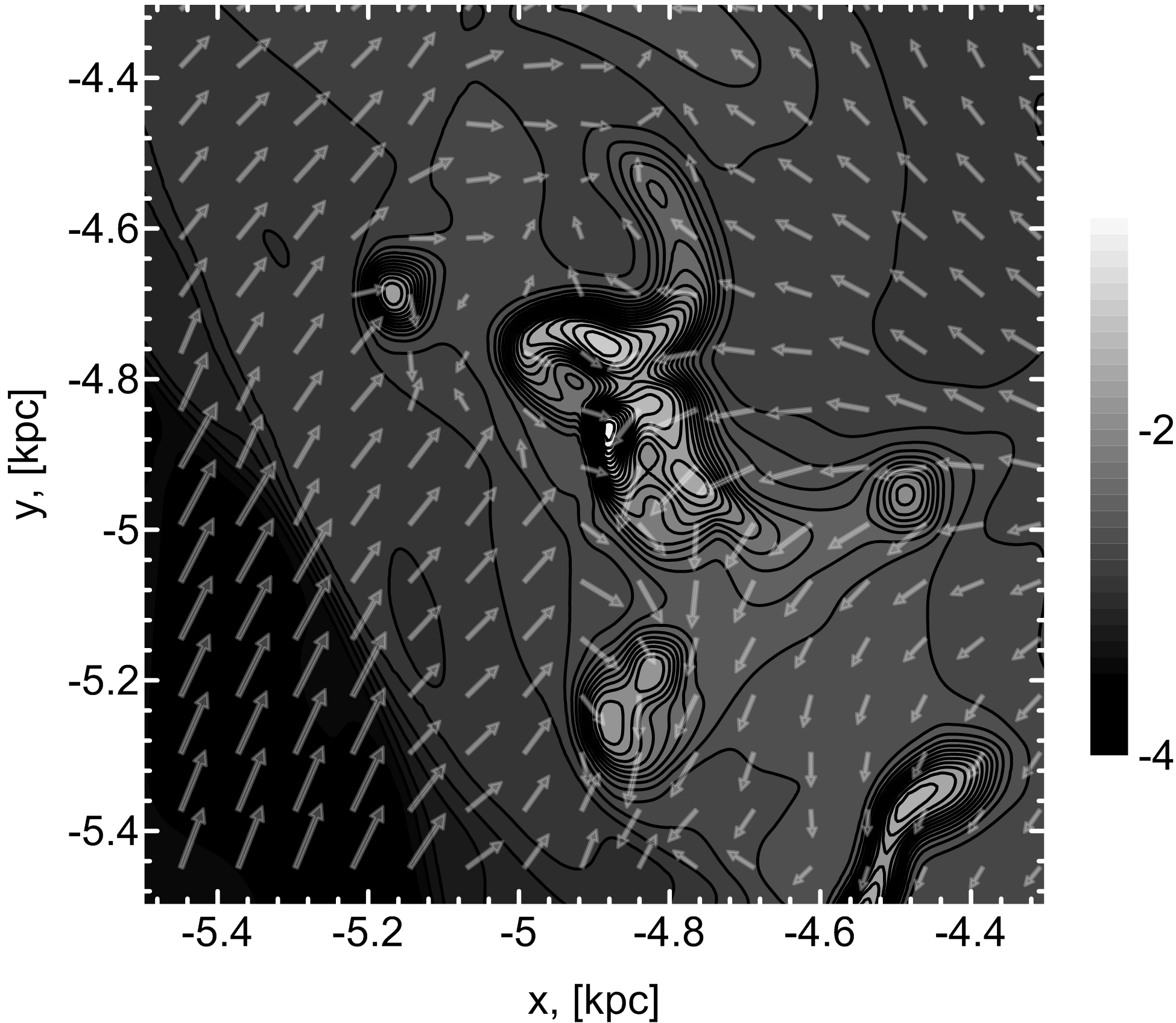
The velocity dispersion in a gas around molecular clouds is about 3-7 km s-1 and the velocity field around clouds shows a complex turbulent structure. To consider this we pick out a cloud with coordinates (-4.9 kpc, -4.9 kpc) at Myr. Figure 3 shows velocity field around such cloud. The velocities are shown in the comoving coordinate system connected to the most dense part of the cloud. One can see the irregular form of the cloud and the colliding gaseous flows in the regions with enhanced density. The structure and physical parameters of the cloud locations obtained in our numerical simulations are close to those observed in the giant molecular clouds and their surroundings (Roman-Duval et al. , 2010).
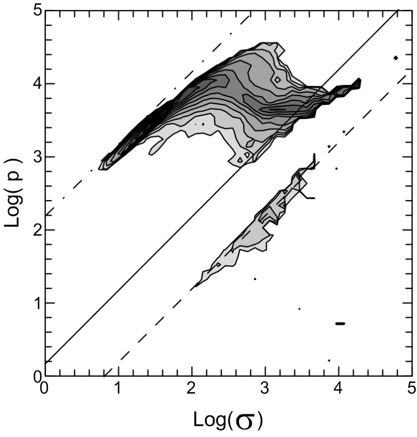
Thermo-chemical processes taken into account in our simulations lead to formation of the two phases of the simulated gas with stable points around K and K (Figure 4, see note on the value of the temperature above)). A gas with K corresponds to the dense molecular clouds, i.e they have both high number density ( cm-3) and high H2 molecule abundance (). These clouds concentrate to the spiral arms. A gas belonging to the warmer phase with K is a rarefied atomic gas which resides mainly between the arms. A gas of the coldest phase ( K) occupies negligibly small volume of space and is not considered here.
4 The physical properties of molecular clouds
In this section we consider physical and statistical properties of the molecular gas in our simulations. This gas resides in the clumps which are called molecular clouds. A border of the cloud can be defined as location where H2 abundance or H2 surface density exceeds given limit. The clouds in our analysis are delimited using a surface density threshold: over the 2D computational grid of the Galactic plane we find isolated groups of cells with the column density exceeding given threshold. Such clumps normally have irregular form, and their effective linear size is estimated as a square root of their surface .
For our analysis we have chosen two values of the molecular hydrogen surface density threshold: g cm-2 and g cm-2. In both cases average density inside a cloud is greater than several dozens particles per cc, which is close to the typical value of H2 number density obtained from observations of molecular clouds in the Galaxy (e.g. Shu et al. , 1987).
We are using two thresholds for H2 surface density at the border of the cloud in order to show that our basic conclusions on the statistical properties of clouds are independent of exact value of the threshold. This is important because there is no single value of H2 surface density which exactly reproduces definition of a molecular cloud in observations.
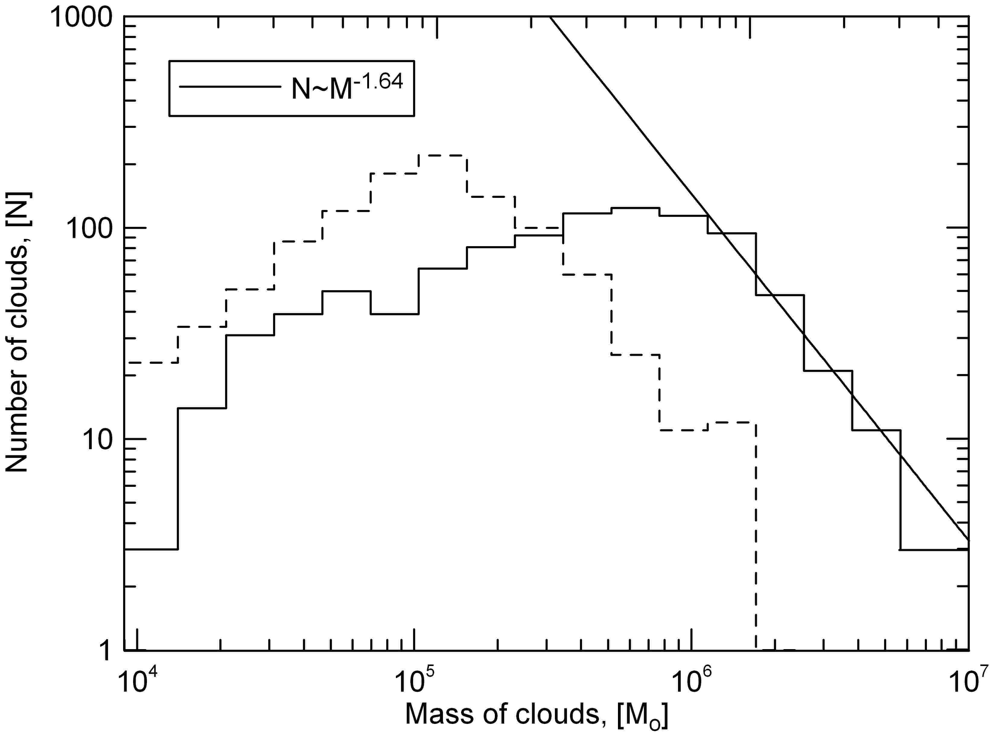
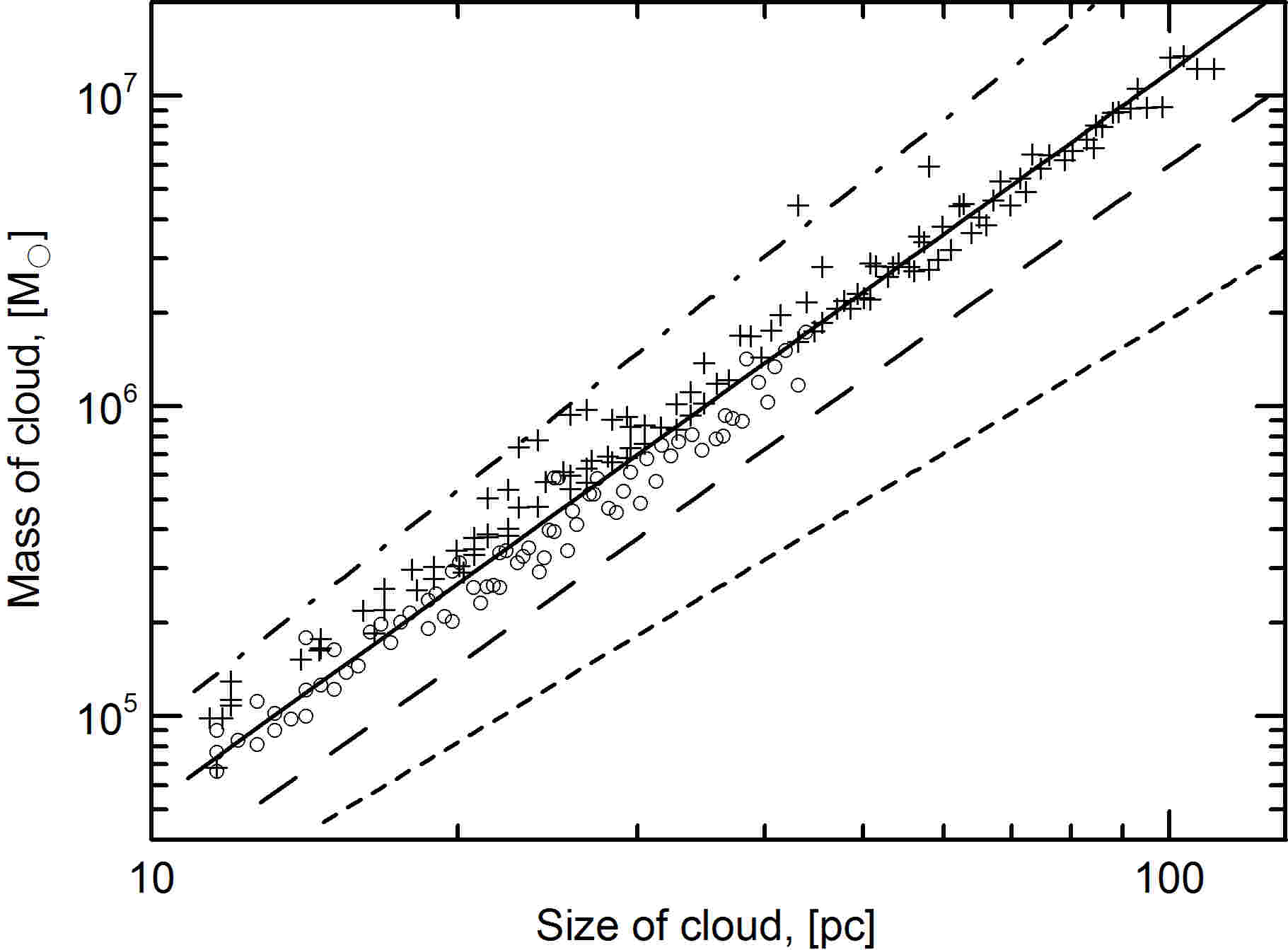
Figure 5 presents the distribution of masses of the clouds for the H2 surface density thresholds g cm-2 (solid line) and g cm-2 (dash line) at Myr.
We find that the spectra of cloud masses for both thresholds follow the power law dependence : in the mass range for the higher threshold value and in mass range for the lower density threshold. This invariance of the spectrum on surface density limit indicates to that physical processes leading to the formation of the structure with density threshold g cm-2 have the same nature. Hence, other statistical properties of the structures should be close. Note that the dependence for the higher threshold is valid in the same mass range as that obtained in the observations of the Galactic molecular clouds (Roman-Duval et al. , 2010). For both thresholds one can see a lack of low-mass clouds. In the case of the higher limit the lack of clouds with can be explained by our numerical resolution, whereas similar deficiency in the observations comes from the incompleteness of the data (Roman-Duval et al. , 2010). For the lower threshold the lack of clouds with can be explained by clustering of smaller and denser clumps. In other words, choosing lower surface density level we pick out more extended clusters of clumps, which contain both smaller and denser clumps. In the case of the lower threshold we cover larger regions with lower density, so that the increase of density limit should lead to decrease of size of the cluster and excludes extended low-density regions from consideration of.
Figure 6 presents the dependence of mass of the cloud on its size (mass-size relationship) for the H2 surface density thresholds g cm-2 (crosses) and g cm-2 (circles) at Myr. The sizes of the clouds vary between pc for the higher density threshold. The most massive clouds have masses about . These values are in good agreement with the observational data (Roman-Duval et al. , 2010). In some cases the sizes of molecular clouds can be as large as pc (Kirsanova et al. , 2008), but these regions can be considered as a tight group of smaller clouds. In our analysis such extended clouds can be found under the lower density threshold (crosses in Figure 6): there are groups or chains of clouds seen in the periphery of the Galaxy at Myr (Figure 2).
The mass-size (or mass-area) relationship among molecular clouds, , which is well-known as Larson’s third law, appears due to cloud evolution and numerous physical processes in the interstellar medium. Many efforts to obtain or explain this universal relation are given in Beaumont et al. (2012), who tried to interpret the relationship in terms of the column density distribution function. However, the scatter of the empirical fits is large (see lines in Figure 6, note that we pick out only several fits from the Table 1 presented in Beaumont et al. , 2012). One can see that the properties of clouds obtained in the numerical simulations are close to the power-law relation between the radius and mass of the cloud , which was obtained by applying a -square minimization for the observed radii and masses of the Galactic molecular clouds (Roman-Duval et al. , 2010). There is a significant dispersion of our simulated data around this fit. We find that our best fit of the simulated data (the ranges correspond different density thresholds) is close to that obtained in observations. Note that our fit has a power-law index close to 2 for both density thresholds considered here.
Finally, we note that the velocity dispersion for the majority of clouds varies in the range km s-1 in our numerical simulations, that is a good agreement with the observational data (Roman-Duval et al. , 2010).
Thus, we have found that the physical properties of clouds obtained from our simulation are close to those observed in the Galaxy. Our conclusions are coinstrained by the numerical resolution, because we can consider clouds with sizes larger than 10 pc, whereas even the parsec-size clouds are observed (Roman-Duval et al. , 2010). Anyhow, our numerical results provide possibility to consider the global properties of molecular and atomic gas in the Galaxy.
5 The diagram
5.1 Molecular hydrogen
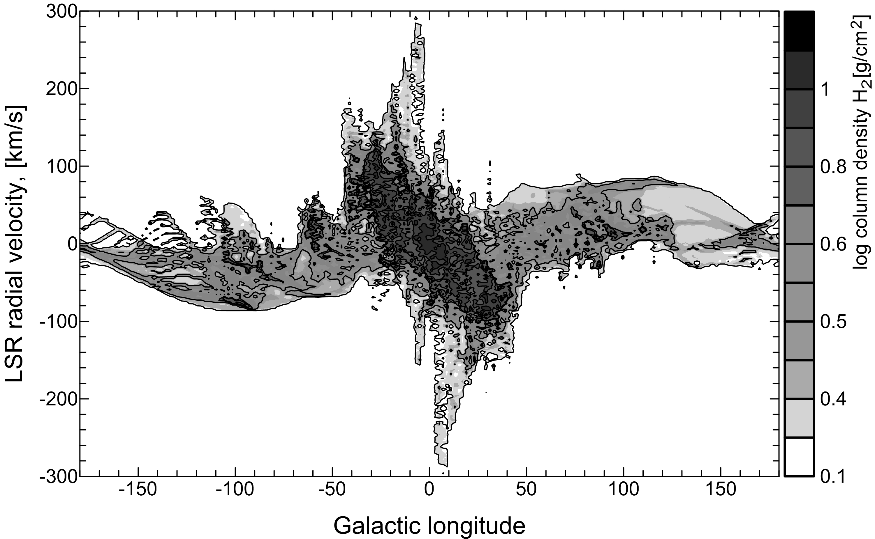
Large-scale distribution of molecular gas in the Galaxy can be represented using the ’longitude-velocity’ diagram (henceforth diagram) constricted from observations of the CO(1-0) line emission (Dame et al. , 2001). The CO molecule is usually used as a tracer of molecular gas (Maloney & Black, 1988) because emission of much more abundant H2 molecule cannot be observed in the cold and warm regions. Current model of molecular kinetics in our simulations does not provide us with possibility to calculate abundance of CO molecule and the distribution of molecular gas is judged from the distribution of H2. Certainly, the CO-H2 conversion factor depends on many physical parameters (Shetty et al. , 2011; Feldmann et al. , 2012). However, there are no doubts that the general conclusion on agreement between synthetic and observational distributions of molecular gas in the Galaxy can be drawn from comparison of diagram for H2 molecule in the model with CO data of Dame et al. (2001).
Figure 7 presents the diagram for molecular gas at Myr. The diagram is constructed for an observer located at the Sun position (see Figure 2). One can find the large-scale structures corresponding to Perseus, Outer and Carina spiral arms. In the central part of the diagram, , an intense and extended structure with the strong velocity gradient that passes through the origin is clearly seen. This structure by its location and general appearance resembles so-called Galactic Molecular Ring (Stecker et al. , 1975; Cohen & Thaddeus, 1977; Roman-Duval et al. , 2010). However, Figure 2 shows that there is no pronounced ring of molecular material in our simulations. In our model the structure in the Molecular Ring locus of points of the diagram is associated with the Galactic bar and the spiral arms at 3-4 kpc. Thus, our results are in agreement with conclusions on the absence of the Molecular Ring drawn from the simple fitting technique Dobbs & Burkert (2012) and previous hydrodynamical simulations (Englmaier & Gerhard, 1999; Rodriguez-Fernandez & Combes, 2008; Baba et al. , 2010). Note that the previous simulations did not include molecular chemical kinetics.
We have to note on the existence of numerous small-scale structures in the diagram. They are obviously associated with spurs, agglomerations of clouds and individual clouds. But we make no comment on that here because our consideration is concentrated on the extended structures scales of which greatly exceed our numerical resolution.
5.2 Atomic hydrogen
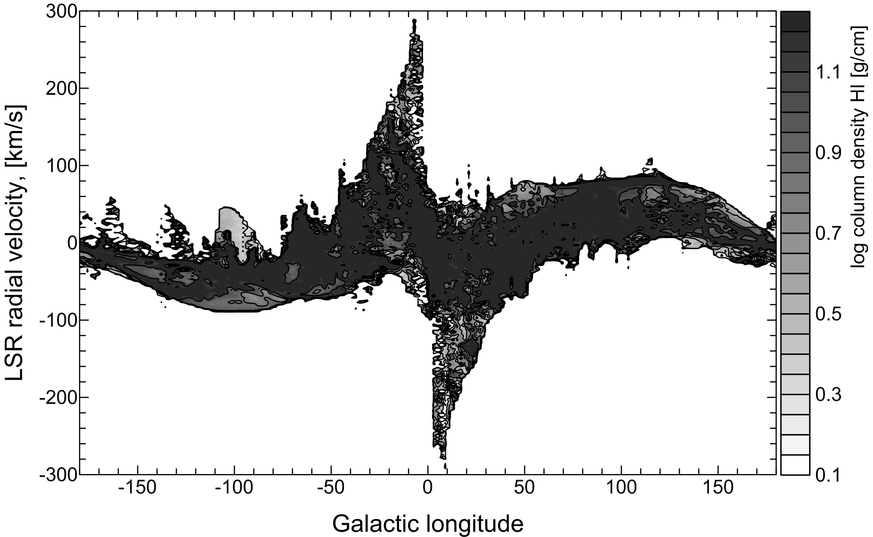
The atomic gas in our model is the main part of the gaseous component of the spiral arms and its distribution traces large-scale structures in the Galaxy. Figure 8 presents the synthetic diagram for atomic gas at Myr. The diagram is constructed for an observer located at the Sun position (see Figure 2). The structures corresponding to the spiral arms are clearly seen in this Figure. The synthetic diagram does not show any prominent structure at the locus of points corresponding to the Galactic Molecular Ring Figure 8). Results of our modelling show that the atomic gas in the simulated Galaxy is distributed much more uniformly than the molecular gas. The synthetic diagram shows reasonably good agreement with the observational data (see, e.g. diagrams in Kalberla & Dedes, 2008; McClure-Griffiths et al. , 2004). So, our model reproduces main features of the observed distribution of the neutral gas in the Galaxy.
6 Conclusion
In this paper we have studied formation of gas clouds in the model of our Galaxy. The 3D simulations have taken into account molecular hydrogen chemical kinetics, cooling and heating processes. Comprehensive gravitational potential have been used. It included contributions of self-gravitating gaseous component, stellar bulge, two and four armed spiral structure, stellar disk and dark halo. We have analyzed general properties of the simulated clouds and have compared them with statistical distributions taken from the recent surveys of molecular clouds (Roman-Duval et al. , 2010).
Our results can be summarized as follows:
-
•
the following stages of evolutionary sequence of the molecular cloud system formation were distinguished in our modelling: a) spurs and fragments (progenitors of molecular clouds) are formed in the spiral arms due to shear and wiggle instabilities at the times Myr; b) numerous molecular clouds start to form after Myr which corresponds to the time scale of molecular hydrogen formation on dust grains; c) a well-developed hierarchical structure of the clouds is formed at Myr; d) at the moment of time Myr the clouds agglomerate into extended associations with sizes exceeding pc while the sizes of individual clouds vary in the range pc;
-
•
the total mass of molecules in the Galaxy increases until Myr, when it saturates; the major part of molecule hydrogen is locked in molecular clouds where the H2 molecule abundance reaches ;
-
•
the statistical dependencies, e.g. the mass spectrum of clouds, the ”mass-size” relation and the velocity dispersion of clouds, obtained in our simulations are close to those observed in the Galaxy (Roman-Duval et al. , 2010);
-
•
the structure is clearly seen in the Galactic Molecular Ring’s locus of points on the simulated diagram of molecular gas; this structure doesn’t correspond to a real ring of molecular gas and likely arises due to superposition of emission from the galactic bar and the spiral arms at 3-4 kpc, which supports conclusion made by (Dobbs & Burkert, 2012); no prominent structure in the Galactic Molecular Ring locus of points is distinguished in the simulated diagram of the HI gas.
7 Acknowledgements
We thank A.V. Zasov and Yu.A. Shchekinov for thoughtful comments on the manuscript. This work was supported partially by Russian Foundation for Basic Research (grants 11-02-12247-ofi-m-2011, 10-02-00231, 12-02-00685-a) and the President of the Russian Federation grant (SS-3602.2012.2). S.A.K. and E.O.V. thank to the foundation ”Dynasty” (Dmitry Zimin) for financial support. E.O.V. thanks to Russian Foundation for Basic Research (grant 11-02-01332). AMS was partly supported by the Russian federal task program Research and operations on priority directions of development of the science and technology complex of Russia for 2007-2012 (state contract 16.518.11.7074). The numerical simulations were made on the supercomputer facilities of NIVC MSU ”Lomonosov” and ”Chebyshev”.
References
- Amores et al. (2009) Amores, E. B.; Lepine, J. R. D.; Mishurov, Yu. N., 2009, MNRAS, 400, 1768
- Asplund et al. (2005) Asplund M., Grevesse N., Sauval A.J., The Solar Chemical Composition. Cosmic Abundances as Records of Stellar Evolution and Nucleosynthesis, 2005, ASP Conf. Ser., 336, eds. T. G. Barnes & F. N. Bash, p.25
- Baba et al. (2010) Baba J., Saitoh T. R., Wada K., 2010, PASJ, 62, 1413
- Bakes & Tielens (1994) Bakes E.L.O., Tielens A.G.G.M., 1994, ApJ, 427, 822
- Ballesteros-Paredes et al. (2007) Ballesteros-Paredes J., Klessen R.S., Mac Low M.-M., Vazquez-Semadeni E., 2007, in Protostars and Planets V, eds. Reipurth B., Jewitt D., and Keil K., University of Arizona Press, p. 63
- Balbus & Cowie (1985) Balbus S. A., Cowie L. L., 1985, ApJ, 297, 61
- Barnes & Hut (1986) Barnes J., Hut. P., 1986, Nature, 324, 446
- Beaumont et al. (2012) Beaumont C.N., Goodman A.A., Alves J.F., Lombardi M., Román-Zúñiga C. G., Kauffmann J., Lada C.J., 2012, MNRAS, in press, arXiv:1204.2557
- Begeman et al. (1991) Begeman K.G., Broeils A.H., Sanders R.H. 1991, MNRAS, 249, 523
- Bergin et al. (2004) Bergin E.A., Hartmann L.W., Raymond J.C., Ballesteros-Paredes J., 2004, ApJ, 612, 921
- Binney & Tremaine (2008) Binney J., Tremaine S., Galactic Dynamics: Second Edition, Princeton University Press, Princeton, 2008, p. 868
- Blitz & Shu (1980) Blitz L., Shu F.H., 1980, ApJ, 238, 148
- Bobylev & Bajkova (2010) Bobylev V.V., Bajkova A.T., 2010, MNRAS, 408, 1788
- Cazaux & Tielens (2004) Cazaux S., Tielens A.G.G.M., 2004, ApJ, 604, 222
- Chou et al. (2000) Chou W., Matsumoto R., Tajima T., Umekawa M., Shibata K., 2000, ApJ, 538, 710
- Cen (1992) Cen R., 1992, ApJ, 78, 341
- Cohen & Thaddeus (1977) Cohen R.S., Thaddeus P., 1977, ApJL, 217, 155
- Cox & Gomez (2002) Cox D.P., Gomez G.C., 2002, ApJS, 142, 261
- Dame et al. (1986) Dame T.M., Elmegreen B.G., Cohen R.S., Thaddeus P., 1986, ApJ, 305, 892
- Dame et al. (2001) Dame T., Hartmann D., Thaddeus P., 2001 ApJ 547, 729
- Draine & Bertoldi (1996) Draine B.T., Bertoldi F., 1996, ApJ, 468, 269
- Dobbs & Bonnel (2006) Dobbs C.L., Bonnell I.A., 2006, MNRAS, 367, 873
- Dobbs et al. (2006) Dobbs C. L., Bonnell I. A., & Pringle J. E., 2006, MNRAS, 371, 1663
- Dobbs & Bonnell (2007a) Dobbs C.L., Bonnell I.A., 2007, MNRAS, 374, 1115
- Dobbs & Bonnell (2007b) Dobbs C.L., Bonnell I.A., 2007, MNRAS, 376, 1747
- Dobbs (2008) Dobbs C.L., 2008, MNRAS, 391, 844
- Dobbs & Burkert (2012) Dobbs C.L. & Burkert A., 2012, MNRAS, 421, 2940
- Efremov (2009) Efremov Y. N., 2009, Astr. Letters 35, 507
- Elmegreen (1979) Elmegreen B. G., 1979, ApJ, 231, 372
- Elmegreen (1994) Elmegreen B. G., 1994, ApJ, 433, 39
- Elmegreen & Falgarone (1996) Elmegreen B., Falgarone E. 1996, ApJ, 471, 816
- Elmegreen (2004a) Elmegreen B.G., 2004, MNRAS 354, 367
- Englmaier & Gerhard (1999) Englmaier P., Gerhard O., 1999, MNRAS, 304, 512
- Falgarone et al. (1992) Falgarone E., Puget J.-L., & Perault M. 1992, A&A, 257, 715
- Feldmann et al. (2012) Feldmann R., Gnedin N.Y., Kravtsov A.V., 2012, ApJ, 747, 124
- Fridman & Khoperskov (2011) Fridman A.M., Khoperskov A.V., Physics of galactic disks, Fizmalit 2011, 640 (in Russian)
- Field & Saslaw (1965) Field G. B., Saslaw W. C., 1965, ApJ, 142, 568
- Galli & Palla (1998) Galli D., Palla F., 1998, A&A, 335, 403
- Goldsmith et al. (1978) Goldsmith P., Langer W.D., 1979, ApJS, 222, 881
- Glover et al. (2010) Glover S.C.O., Federrath C., Mac Low M.-M., Klessen R.S., 2010, MNRAS, 404, 2
- Glover & Mac Low (2011) Glover S. C. O., & Mac Low M., 2011, MNRAS, 412, 337
- Habing (1968) Habing H.J., 1968, BAIN, 19, 421
- Heyer et al. (2009) Heyer M., Krawczyk C., Duval J., & Jackson J. M. 2009, ApJ, 699, 1092
- Hollenbach & McKee (1979) Hollenbach D., McKee C.F., 1979, ApJS, 41, 555
- Hollenbach & McKee (1989) Hollenbach D., McKee C.F., 1989, ApJ, 342, 306
- Kalberla & Dedes (2008) Kalberla P.M.W., Dedes L., 2008, A&A, 487, 951
- Kauffmann et al. (2010) Kauffmann J., Pillai T., Shetty R., Myers P. C., & Goodman A. A. 2010, ApJ, 712, 1137
- Khoperskov & Tiurina (2003) Khoperskov A.V, Tyurina N. V. 2003, ARep, 47, 443
- Kirsanova et al. (2008) Kirsanova M.S., Sobolev A.M., Thomasson M., Wiebe D.S., Johansson L.E.B., Seleznev A.F., 2008, MNRAS 388, 729
- Kim & Ostriker (2006) Kim W.-T., Ostriker E. C., 2006, ApJ, 646, 213
- Kwan & Valdes (1987) Kwan J., Valdes F., 1987, ApJ, 315, 92
- Lada & Lada (2003) Lada C.J., Lada E.A., 2003, ARA&A, 41, 57
- Lada et al. (2008) Lada, C. J., Muench, A. A., Rathborne, J., Alves, J. F., & Lombardi, M. 2008, ApJ, 672, 410
- Larson (1981) Larson R.B., 1981, MNRAS, 194, 809
- Lepine et al. (2001) Lepine J.R.D., Mishurov Yu.N., Dedikov S.Yu., 2004, ApJ, 546, 234
- Levinson & Roberts (1981) Levinson F. H., Roberts Jr. W. W., 1981, ApJ, 245, 465
- MacLow & Shull (1986) Mac Low M.-M., Shull J.M., 1986, ApJ, 302, 585
- Maloney & Black (1988) Maloney P., Black J.H., 1988, ApJ, 325, 389
- McClure-Griffiths et al. (2004) McClure-Griffiths N.M., Dickey J.M., Gaensler B.M., Green A.J., 2004, ApJL, 607, 127
- McKee & Ostriker (2007) McKee C.F., Ostriker E.C., 2007, ARA&A, 45, 565
- Mishurov & Suchkov (1975) Mishurov I.N., Suchkov A.A., 1975, ApSS, 35, 285
- Nelson & Matsuda (1977) Nelson A.H., Matsuda T., 1977, MNRAS, 179, 663
- Rathborne et al. (2009) Rathborne J.M., Johnson A.M., Jackson J.M., Shah R.Y., Simon R., 2009, ApJS, 182, 131
- Roberts (1969) Roberts W.W., 1969, ApJ, 158, 123
- Roberts & Stewart (1987) Roberts W. W., Stewart G. R., 1987, ApJ, 314, 10
- Rodriguez-Fernandez & Combes (2008) Rodriguez-Fernandez N. J., Combes F., 2008, A&A, 489, 115
- Román-Zúñiga et al. (2010) Román-Zúñiga C. G., Alves J. F., Lada C. J., & Lombardi M. 2010, ApJ, 725, 2232
- Roman-Duval et al. (2010) Roman-Duval J., Jackson J. M., Heyer M., Rathborne J., Simon R., 2010, ApJ, 723, 492
- Shetty & Ostriker (2006) Shetty R., Ostriker E.C., 2006, ApJ, 647, 997
- Shetty et al. (2011) Shetty R., Glover S.C., Dullemond C.P., Ostriker E.C., Harris A.I., Klessen R.S., 2011, MNRAS, 415, 3253
- Shu et al. (1987) Shu F.H., Adams F.C., Lizano S., 1987, ARA&A, 25, 23
- Sofue et al. (2009) Sofue Y., Honma M., Omodaka T., 2009, PASJ, 61, 227
- Solomon et al. (1987) Solomon P. M., Rivolo A. R., Barrett J., & Yahil A. 1987, ApJ, 319, 730
- Spitzer (1953) Spitzer L., 1953, ApJ 118, 106
- Stecker et al. (1975) Stecker F.W., Solomon P.M., Scoville N.Z., Ryter C.E., 1975, ApJ, 201, 90
- Sutherland & Dopita (1993) Sutherland R.S., Dopita M.A., 1993, ApJS, 88, 253
- Tasker & Tan (2009) Tasker E.J., & Tan J.C., 2009, ApJ, 700, 358
- Tielens & Hollenbach (1985) Tielens A.G.G.M, Hollenbach D., 1985, ApJ 291, 722
- Tomisaka (1984) Tomisaka K., 1984, PASJ, 36, 457
- van Leer (1979) van Leer B., 1979, Journ. Comput. Phys., 32, 101
- Wada (1994) Wada. K., 1994, PASJ, 46, 165
- Wada et al. (2000) Wada K., Spaans M., Kim S., 2000, ApJ, 540, 797
- Wada (2001) Wada K., 2001, ApJL., 559, 41
- Wada & Koda (2004) Wada K. & Koda J., 2004, MNRAS, 349, 270
- Wolfire et al. (2003) Wolfire M.G., McKee C.F., Hollenbach D., Tielens A.G.G.M., 2003, ApJ, 587, 278
- Zhang & Song (1999) Zhang T. J. & Song G. X., 1999, Ap&SS, 266, 521
Appendix A External gravitational potential model
The dark matter halo gravitational potential is taken in the quasi-isothermal form (Begeman et al. , 1991):
| (9) |
where , is the mass of the dark halo within a radius , is the scale of the halo and . In our model we take kpc, kpc, .
For the stellar bulge potential we adopt the King’s model with the cutoff at radius (Fridman & Khoperskov, 2011)
| (10) |
with the following parameters , kpc, kpc, where
For the three-dimensional stellar disk we take the exponential distribution of surface density, then the stellar disk potential can be written as follows (Binney & Tremaine, 2008)
| (11) |
where , is the central surface density, , the radial scale of disk kpc, the vertical scale pc, are the cylindrical Bessel functions of the first and second kind, respectively.
Taking account the gravitational potentials of bar and spiral structure of stellar component we can obtain more realistic distribution of gas in the Galaxy. Following Cox & Gomez (2002) the perturbed potential of stellar disk can be written in the form of superposition of potentials generated by the bar and the two and four-armed logarithmic spiral patterns:
| (12) |
where describes the evolution of the relative amplitude of the spiral stellar density wave. We assume a linear increase of the amplitude during Myr, after that time the amplitude is constant: .
The relative perturbation is adopted in the form (Wada & Koda, 2004):
| (13) |
where , , ; kpc, kpc, kpc are the radial scales for bar, two-armed and four-armed spiral patterns, respectively. The functions are:
are the phases of bar and spiral patterns, kpc, are the scales and the pitch angles of two-armed and four-armed components.