Actions for axisymmetric potentials

Abstract

We give an algorithm for the economical calculation of angles and actions for stars in axisymmetric potentials. We test the algorithm by integrating orbits in a realistic model of the Galactic potential, and find that, even for orbits characteristic of thick-disc stars, the errors in the actions are typically smaller than 2 percent. We describe a scheme for obtaining actions by interpolation on tabulated values that significantly accelerates the process of calculating observables quantities, such as density and velocity moments, from a distribution function.

1 Introduction

When electronic computers first became widely available, it was discovered that orbits in typical axisymmetric galactic potentials usually admit three isolating integrals of motion (Henon & Heiles, 1964; Ollongren, 1965). Consequently, by Jeans’ theorem, the distribution functions (dfs) of equilibrium axisymmetric galaxies should be functions of three integrals of motion. Unfortunately, analytic forms of all three integrals are known only for exceptional potentials, so the few three-dimensional galaxy models in the literature that have a known df (e.g. Rowley, 1988) employ only the classical energy and angular-momentum integrals $E$ and $L_{z}$, and therefore lack generality.

The action integrals $J_{r}$, $J_{z}$ and $L_{z}$ are particularly useful constants of motion (e.g. Binney, 2012), and we have previously argued the merits of models in which the distribution function is an analytic function of $J_{r}$, $J_{z}$ and $L_{z}$. To take advantage of these models one should be able to evaluate economically the actions of a star from its conventional phase-space coordinates $({\bf x},{\bf v})$. To date we have used two techniques for evaluating actions: (i) torus construction (Kaasalainen & Binney, 1994; Binney & McMillan, 2011) and (ii) the adiabatic approximation (Binney, 2010; Binney & McMillan, 2011; Schönrich & Binney, 2012). Torus construction is a general and rigorous technique and for some applications it is the technique of choice (e.g. McMillan & Binney, 2012). For other applications it is inconvenient because it delivers $({\bf x},{\bf v})$ as functions of the actions and angles, rather than the actions and angles as functions of $({\bf x},{\bf v})$.

The adiabatic approximation delivers actions and angles as functions of $({\bf x},{\bf v})$ but it is reasonably accurate only for stars that stay close to the Galaxy’s mid-plane. Here we introduce a different approximate way to obtain actions, which, though still approximate, is more accurate than the adiabatic approximation and is valid for stars that move far from the mid plane.

2 The algorithm

Our algorithm is based on the idea that the Galaxy’s gravitational potential is similar to a Stäckel potential – for a detailed description of the latter see de Zeeuw (1985). Stäckel potentials for oblate bodies are framed in terms of prolate confocal coordinates. The latter are defined by the distance $2\Delta$ between the foci of the coordinate curves. These foci lie at $R=0$ and $z=\pm\Delta$, where $(R,z,\phi)$ is a system of cylindrical polar coordinates. Following Binney & Tremaine (2008; hereafter BT08) §3.5.3 we define new coordinates $(u,v)$ by

$$R=\Delta\sinh u\sin v\quad;\quad z=\Delta\cosh u\cos v.$$ (1)

The generating function of the canonical transformation between these systems of coordinates is

$$S(p_{R},p_{z},u,v)=p_{R}R(u,v)+p_{z}z(u,v)$$ (2)

so from $p_{u}=\partial S/\partial u$ we have

$$p_{u} = \Delta(p_{R}\cosh u\sin v+p_{z}\sinh u\cos v)$$

$$p_{v} = \Delta(p_{R}\sinh u\cos v-p_{z}\cosh u\sin v).$$ (3)

In these coordinates a Stäckel potential can be written in terms of two functions of one variable, $U(u)$ and $V(v)$, being given by

$$\Phi_{\rm S}(u,v)={U(u)-V(v)\over\sinh^{2}u+\sin^{2}v}.$$ (4)

This being so, the Hamilton–Jacobi equation yields (BT08 eq. 3.249)

$${p_{u}^{2}\over 2\Delta^{2}} = E\sinh^{2}u-I_{3}-U(u)-{L_{z}^{2}\over 2\Delta^{2}\sinh^{2}u}$$

$${p_{v}^{2}\over 2\Delta^{2}} = E\sin^{2}v+I_{3}+V(v)-{L_{z}^{2}\over 2\Delta^{2}\sin^{2}v},$$ (5)

where $E$ is the orbit’s energy and $I_{3}$ is a constant of separation. These equations make $p_{u}(u)$ and $p_{v}(v)$ functions of only their conjugate coordinate, so we can evaluate the actions as

$$J_{r}={1\over\pi}\int_{u_{\rm min}}^{u_{\rm max}}{\rm d}u\,p_{u}(u)\quad;\quad J_{z}={2\over\pi}\int_{v_{\rm min}}^{\pi/2}{\rm d}v\,p_{v}(v),$$ (6)

where $u_{\rm min}\leq u_{\rm max}$ are the roots of $p_{u}(u)=0$ and $v_{\rm min}$ is the root of $p_{v}(v)=0$. Note that an orbit’s actions are independent of any system of coordinates and the subscripts $r$ and $z$ on the actions merely remind us that, in a general way, $J_{r}$ quantifies oscillations inwards and outwards, while $J_{z}$ quantifies oscillations around the equatorial plane.

In as much as our potential $\Phi$ is similar to a Stäckel potential, we have

$$(\sinh^{2}u+\sin^{2}v)\Phi(u,v)\simeq U(u)-V(v).$$ (7)

Consequently, we have

$$\delta U \equiv (\sinh^{2}u+\sin^{2}v)\Phi(u,v)-(\sinh^{2}u_{0}+\sin^{2}v)\Phi(u_{0},v)$$

$$\simeq U(u)-U(u_{0})$$

$$\delta V \equiv \cosh^{2}u\Phi(u,\pi/2)-(\sinh^{2}u+\sin^{2}v)\Phi(u,v)$$

$$\simeq V(v)-V(\pi/2).$$

Here $u_{0}$ is a reference value of $u$, the choice of which will be discussed below, and the right side of the first equation appears to be a function of $v$ but its dependence on $v$ will be weak unless $\Phi$ is very unlike a Stäckel potential. Similarly, we assume that the dependence of the right side of the second equation on $u$ is at most weak. Then, given a point $({\bf x},{\bf v})$ on the orbit we can calculate two constants of motion:

$$I_{3}+U(u_{0}) \simeq I_{3}+U(u)-\delta U(u)$$

$$= E\sinh^{2}u-{p_{u}^{2}\over 2\Delta^{2}}-{L_{z}^{2}\over 2\Delta^{2}\sinh^{2}u}-\delta U(u)$$

$$I_{3}+V(\pi/2) \simeq I_{3}+V(v)-\delta V(v)$$

$$= {p_{v}^{2}\over 2\Delta^{2}}-E\sin^{2}v+{L_{z}^{2}\over 2\Delta^{2}\sin^{2}v}-\delta V(v).$$

Now we can evaluate $p_{u}$ for any given $u$ from

$${p_{u}^{2}\over 2\Delta^{2}}\simeq E\sinh^{2}u-[I_{3}+U(u_{0})+\delta U(u)]-{L_{z}^{2}\over 2\Delta^{2}\sinh^{2}u},$$ (10)

so we can evaluate the integral for $J_{r}$. The integral for $J_{z}$ is evaluated in the same way.

In principle $u_{0}$ can be taken to be any quantity that is constant along an orbit, but the accuracy of our work will depend on our choosing a value such that the term in the definition (2) of $\delta U$ that contains $u_{0}$ almost completely eliminates the $v$ dependence of the first term in this equation. In fact, the natural choice for $u_{0}$ is the location $\overline{u}$ of the minimum with respect to $u$ of $\delta U$ at fixed $v$. This minimum can be determined before we have specified $u_{0}$ because the derivative with respect to $u$ of the first of equations (2) is manifestly independent of $u_{0}$. Physically $\overline{u}$ is the radial coordinate of the shell orbit $J_{r}=0$ of given values of $E$ and $L_{z}$.

2.1 Angle variables

Equations (2) for the momenta are obtained by solving the Hamilton–Jacobi equation for the generating function $S(u,v,\phi,J_{r},J_{z},L_{z})$ of the canonical transformation between the $(u,v,\phi,p_{u},\ldots)$ and the $(\theta_{r},\theta_{z},\theta_{\phi},J_{r},\ldots)$ systems of canonical coordinates with $S$ of the form

$$S=S_{u}(u,J_{r},J_{z},L_{z})+S_{v}(v,J_{r},J_{z},L_{z})+\phi L_{z}.$$ (11)

Given that $S$ takes this form, we may write

$$S = \int{\rm d}u\,{\partial S_{u}\over\partial u}+\int{\rm d}v\,{\partial S_{v}\over\partial v}+\int{\rm d}\phi\,{\partial S\over\partial\phi}$$ (12)

$$= \int{\rm d}u\,p_{u}+\int{\rm d}v\,p_{v}+\phi L_{z}$$

Hence

$$\theta_{r} = {\partial S\over\partial J_{r}}=\int{\rm d}u\,{\partial p_{u}\over\partial J_{r}}+\int{\rm d}v\,{\partial p_{v}\over\partial J_{r}}$$

$$\theta_{z} = {\partial S\over\partial J_{z}}=\int{\rm d}u\,{\partial p_{u}\over\partial J_{z}}+\int{\rm d}v\,{\partial p_{v}\over\partial J_{z}}$$ (13)

$$\theta_{\phi} = {\partial S\over\partial L_{z}}=\int{\rm d}u\,{\partial p_{u}\over\partial L_{z}}+\int{\rm d}v\,{\partial p_{v}\over\partial L_{z}}+\phi.$$

We obtain the derivatives of $p_{u}$ and $p_{v}$ from the chain rule. For example

$${\partial p_{u}\over\partial J_{r}} = {\partial p_{u}\over\partial E}{\partial E\over\partial J_{r}}+{\partial p_{u}\over\partial I_{3}}{\partial I_{3}\over\partial J_{r}}$$ (14)

$$= {\partial p_{u}\over\partial E}\Omega_{r}+{\partial p_{u}\over\partial I_{3}}{\partial I_{3}\over\partial J_{r}},$$

where $\Omega_{r}=\partial E/\partial J_{r}$ is the radial frequency, so

$${\theta_{r}\over\surd 2\Delta} = \Omega_{r}\left(\int_{u_{\rm min}}^{u}{\rm d}u\,{\sinh^{2}u\over p_{u}}+\int_{v_{\rm min}}^{v}{\rm d}v\,{\sin^{2}v\over p_{v}}\right)$$ (15)

$$-{\partial I_{3}\over\partial J_{r}}\left(\int_{u_{\rm min}}^{u}{{\rm d}u\over p_{u}}-\int_{v_{\rm min}}^{v}{{\rm d}v\over p_{v}}\right).$$

A detail possibly worth noting is that we always take $p_{u}$ of $p_{v}$ to be given by the positive square root and when considering a point in phase space at which $p_{u}<0$ we obtain the indefinite integrals over $u$ as twice the corresponding integral from $u_{\rm min}$ to $u_{\rm max}$ minus the integral from $u_{\rm min}$ to $u$ with $p_{u}$ taken to be positive. When this procedure is followed for all integrals, the angle variables increase along an orbit continuously as they should.

The derivatives with respect to $J_{r}$ in equation (14) can be obtained by observing that by the chain rule the matrix

$$\pmatrix{\Omega_{r}&\Omega_{z}&\Omega_{\phi}\cr\partial I_{3}/\partial J_{r}&\partial I_{3}/\partial J_{z}&\partial I_{3}/\partial L_{z}\cr 0&0&1}$$ (16)

is the inverse of the matrix

$$\pmatrix{\partial J_{r}/\partial E&\partial J_{r}/\partial I_{3}&\partial J_{r}/\partial L_{z}\cr\partial J_{z}/\partial E&\partial J_{z}/\partial I_{3}&\partial J_{z}/\partial L_{z}\cr 0&0&1}.$$ (17)

The latter is readily obtained by differentiating equations (6) and leads to the definite integrals mentioned in the previous paragraph.

2.2 Interpolation

To recover the observable properties of a model stellar system at a given spatial point, such as its density $\rho$ and velocity dispersion tensor $\sigma^{2}_{ij}$, one has to integrate the distribution function over all velocities. These integrals entail large numbers of evaluations of the df, and it is important to keep down the cost of each evaluation. This goal motivates us to tabulate the values of $J_{r}$ and $J_{z}$ as functions of the classical integrals $E$, $L_{z}$ and $I_{3}+U(u_{0})$ or $I_{3}+V(\pi/2)$. However, $I_{3}+U(u_{0})$ proves ill-suited to this task because its numerical value varies rapidly as one moves through action space. A more convenient constant of motion is

$$E_{r} \equiv {p_{u}^{2}\over 2\Delta^{2}}+{L_{z}^{2}\over 2\Delta^{2}}\left({1\over\sinh^{2}u}-{1\over\sinh^{2}u_{0}}\right)+\delta U(u)$$ (18)

$$\qquad-E(\sinh^{2}u-\sinh^{2}u_{0}).$$

At $u=u_{0}$, which we have chosen to be the minimum of the potential that governs the motion in $u$, $E_{r}=p_{u}^{2}/2\Delta^{2}$ so we can think of $E_{r}$ as the energy invested in radial oscillations. Consequently, for any values of $E$ and $L_{z}$, $E_{r}$ vanishes for $J_{r}=0$ and takes its largest value for $J_{z}=0$ and we can readily obtain $J_{r}$ and $J_{z}$ by interpolating between the values taken by $J_{r}$ and $J_{z}$ at a grid of values of $E_{r}$.

In detail we structure the grid in $(L_{z},E,E_{r})$ space as follows. The grid points in $L_{z}$ are defined by the angular momenta of circular orbits with radii uniformly distributed between minimum and maximum radii. For each value of $L_{z}$ we adopt as grid points in $E$ the energies

$$E_{i}=E_{c}(L_{z})+\left({i\over 2N}v_{\rm max}\right)^{2},$$ (19)

where $E_{c}(L_{z})$ is the energy of the circular orbit with angular momentum $L_{z}$ and ${\textstyle{1\over 2}}v_{\rm max}^{2}$ is slightly smaller than the difference between the energy of that orbit and the escape energy from its circle. For each such energy we identify $u_{0}=\overline{u}$, the minimum with respect to $u$ of

$$E\sinh^{2}u-\delta U-L_{z}^{2}/(2\Delta^{2}\sinh^{2}u).$$ (20)

Then we find the speed $v$ that the star has at this spatial point and determine the values taken by $E_{r}$, $I_{3}+V(\pi/2)$, $J_{r}$ and $J_{z}$ at the phase-space point $({\bf x},{\bf v})=(\Delta\sinh(u_{0}),0,v\cos\psi,v\sin\psi)$ for values of $\psi$ uniformly distributed in $(0,\pi/2)$. With this scheme interpolation errors can be kept below $\sim 1\%$ with a grid of size $60\times 50\times 50$, which takes $\sim 30\,$sec to compute on a laptop.

The present algorithm lends itself to tabulation better than the adiabatic approximation because with the present algorithm it is straightforward to resort to the algorithm whenever actions are required for values of the integrals that lie outside the grid. By contrast, when the adiabatic approximation is used, values of $E_{z}$ are required for given $J_{z}$ and these are hard to obtain beyond the limits of the pre-computed table of values of $J_{z}$ for given $E_{z}$.

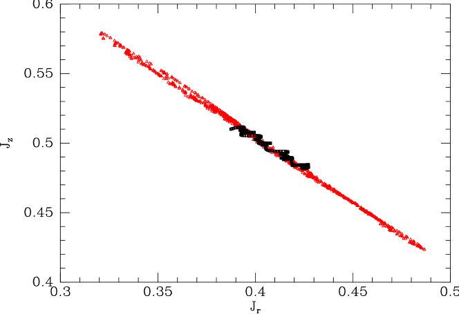
Figure 1: Top: values of $J_{r}$ and $J_{z}$ recovered along an orbit in a realistic Galactic potential. The black points are obtained with the algorithm of Section 2 using $\Delta=3.5\,{\rm kpc}$ while the red points are obtained with the adiabatic approximation. The units are $100\,{\rm km}\,{\rm s}^{-1}\,{\rm kpc}$. Bottom: the evolution of the angle variables along this orbit.

3 tests

We have tested the algorithm by numerically integrating orbits in a realistic Galaxy potential and after each time-step using the above algorithm to determine $(\theta_{r},\theta_{z},J_{r},J_{z})$. Any variation in the recovered values of the actions along the orbit quantifies errors in the procedure, as do deviations of the motion in the $(\theta_{r},\theta_{z})$ lane from straight lines. The adopted potential is that of model 2 of Dehnen & Binney (1998) modified to give the thin disc a scale height of $0.3\,{\rm kpc}$ – this potential is generated by exponential thin and thick stellar discs, plus a gas disc, an axisymmetric bulge with axis ratio $0.6$ and a dark halo with axis ratio $0.8$. The upper panel of Fig. 1 shows values of the actions along an orbit that has corners at $(R,z)=(9.5,2)\,{\rm kpc}$ and $(6.6,1.35)\,{\rm kpc}$. The black points are obtained using the above algorithm, while the red points are obtained with the adiabatic approximation in the superior formulation of Schönrich & Binney (2012). Quantitatively, with the adiabatic approximation the standard deviations of $J_{r}$ and $J_{z}$ are $(4.13,3.89)\,{\rm km}\,{\rm s}^{-1}\,{\rm kpc}$ while with the above algorithm they are $(1.16,0.97)\,{\rm km}\,{\rm s}^{-1}\,{\rm kpc}$, smaller by a factor $\sim 4$. The lower panel shows the values taken by $(\theta_{r},\theta_{z})$ at each integration step. The points lie on straight lines as required and the slopes of plots of $\theta_{i}$ versus time agree accurately with the frequencies that are recovered from the formulae of Section 2.

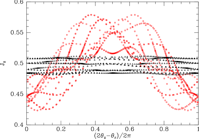
Figure 2: $J_{z}$ in units of $100\,{\rm km}\,{\rm s}^{-1}\,{\rm kpc}$ versus the combination of angle variables $2\theta_{z}-\theta_{r}$ along the orbit that gives rise to Fig. 1. The black triangles are obtained with the algorithm of Section 2 while the red squares are obtained with the adiabatic approximation.

Since the upper panel of Fig. 1 shows that the actions we recover, either by the present algorithm or from the adiabatic approximation, are tightly correlated, it is natural to ask what else they are correlated with. Their correlations with $R$ and $z$ prove to be extremely small (especially in the case of the present algorithm), but the red squares in Fig. 2 show that in the case of the adiabatic approximation $J_{z}$ (and therefore $J_{r}$ also) is correlated with the combination of angle variables $2\theta_{r}-\theta_{z}$. This angular dependence implies that as one moves over an orbital torus at constant radius, the error in $J_{z}$ has one sign in the plane and another far from it, and that the magnitude of this pattern of errors oscillates between pericentre and apocentre, changing sign somewhere in between. The black triangles in Fig. 2 show that the present algorithm yields more accurate actions largely by eliminating this angular dependence.

Figure 3: The ratios of the standard deviations in $J_{r}$ and $J_{z}$ to $(J_{r}+J_{z})/2$ as functions of the maximum distance from the plane attained on the orbit. Along this sequence of orbits $J_{z}$ rises from zero to $240\,{\rm km}\,{\rm s}^{-1}\,{\rm kpc}$, while $J_{r}$ decreases from $50$ to $25\,{\rm km}\,{\rm s}^{-1}\,{\rm kpc}$.

Fig. 3 plots the ratios of the standard deviations of $J_{r}$ and $J_{z}$ to $(J_{r}+J_{z})/2$ as functions of the maximum height $z_{\rm max}$ attained on the orbit – all orbits were started by dropping particles from $(R,z)=(9.5\,{\rm kpc},z_{\rm max})$. The fractional error in $J_{z}$ is never more than 4% and is rarely in excess of 2%. The error in $J_{r}$ is larger but is still generally under 2% of the average action. The pronounced peaks in the errors in both actions around $z_{\rm max}=2.5\,{\rm kpc}$ is probably connected with the $1:1$ resonance between the horizontal and vertical motions: none of the orbits contributing to the figure appears to be actually trapped, but for $z_{\rm max}\sim 2.6\,{\rm kpc}$ the frequency $\Omega_{r}-\Omega_{z}$ is very low. Consequently, the small difference between $\Phi$ and a Stäckel potential has appreciable time to disturb the orbit.

Figure 4: The points above $\hbox{SD/J}=0.03$ show standard deviations of $J_{r}$ (triangles) and $J_{z}$ (squares), normalised by $(J_{r}+J_{z})/2$, along the orbit that yielded Fig. 1 as functions of the value of $\Delta$ used in the algorithm. The lower points show the corresponding numbers for an orbit that has its outer corner at $(R,z)=(9.5,1)\,{\rm kpc}$ rather than $(9.5,2)\,{\rm kpc}$. The latter orbit has actions $(45.7,15.6)\,{\rm km}\,{\rm s}^{-1}\,{\rm kpc}$.

The results shown in Figs. 1 to 3 were obtained with $\Delta=3.5\,{\rm kpc}$. Fig. 4 shows the standard deviations of $J_{r}$ and $J_{z}$ along two orbits as functions of $\Delta$. The orbits have similar eccentricities, but different values of $z_{\rm max}$: the upper squares and triangles are associated with an orbit that has $z_{\rm max}=2\,{\rm kpc}$, while the lower triangles and points are for an orbit that has $z_{\rm max}=1\,{\rm kpc}$. Both orbits have corners at $R\sim 9.5$ and $\sim 6.5\,{\rm kpc}$. We see that the standard deviation in the values of $J_{z}$ along the orbit is much less sensitive to the value of $\Delta$ than is the standard deviation of the $J_{r}$ values.

4 Conclusions

We have shown that values of actions and angles accurate to a couple of percent can be obtained for orbits in a realistic axisymmetric model of the Galactic potential by treating the potential as if it were a Stäckel potential. For orbits typical of observed stars belonging to either the thin or thick discs the error in $J_{z}$ is always less than $\sim 4\%$ of the average action and is usually significantly smaller. The errors in $J_{r}$ are always less than 6% and usually less than 2% of the average action. Even in the era of Gaia it is unlikely that the errors in the measured phase-space coordinates of any star will be small enough that the inaccuracies inherent in our algorithm will dominate the final uncertainties in derived angles and actions. The errors in actions obtained from the adiabatic approximation are larger by a factor $\sim 4$ for thin-disc stars and significantly larger still for thick-disc stars.

A possibility that we have not pursued, but which might be important if one needs to model an entire galaxy rather than the extended solar neighbourhood, is to make the inter-focal semi-distance $\Delta$ a function of $L_{z}$ and $E$ – by integrating a few orbits at wide-ranging values of $L_{z}$ and $E$ it should be possible to choose a suitable functional form for $\Delta(L_{z},E)$.

Each action evaluation requires a one-dimensional integral and with the existing code takes $\sim 100\,\mu{\rm s}$ on a laptop. Each angle evaluation takes about twice as long because it requires of order two one-dimensional integrals. Since evaluation of the observables that follow from a df requires a great many evaluations of the actions, it is cost-effective to tabulate $(J_{r},J_{z})$ as functions of the classical integrals $(L_{z},E,I_{3})$ and we have described an effective scheme for doing this. In a companion paper we illustrate what can be achieved using this scheme by fitting dfs to observational data for our Galaxy.

References

- Binney (2010) Binney J., 2010, MNRAS, 401, 2318 (B10)
- Binney (2012) Binney, J., 2012, arXiv1202.3403
- Binney & McMillan (2011) Binney J., McMillan P.J., 2011, MNRAS, 413, 1889
- Binney & Tremaine (2008) Binney J., Tremaine S., 2008, “Galactic Dynamics”, Princeton University Press, Princeton
- Dehnen & Binney (1998) Dehnen W., Binney J., 1998, MNRAS, 298, 387
- de Zeeuw (1985) De Zeeuw P.T., 1985, MNRAS, 216, 273
- Henon & Heiles (1964) Henon M., Heiles C., 1964, AJ, 69, 73
- Kaasalainen & Binney (1994) Kaasalainen M., Binney J., 1994, MNRAS, 268, 1033
- McMillan & Binney (2012) McMillan P.J., Binney, J., 2012, MNRAS, 419, 2251
- Ollongren (1965) Ollongren A., 1965, ARA&A, 3, 113
- Rowley (1988) Rowley G., 1988, ApJ, 331, 124
- Schönrich & Binney (2012) Schönrich R., Binney J., 2012, MNRAS, 419, 1546