Consequences of moduli stabilization in the Einstein-Maxwell landscape

Abstract

A toy landscape sector is introduced as a compactification of the Einstein-Maxwell model on a product of two-spheres. Features of the model include: moduli stabilization, a distribution of the effective cosmological constant of the dimensionally reduced 1+1 spacetime, which is different from the analogous distribution of the Bousso-Polchinski landscape, and the absence of the so-called $\alpha^{*}$-problem. This problem arises when the Kachru-Kallosh-Linde-Trivedi stabilization mechanism is naively applied to the states of the Bousso-Polchinski landscape. The model also contains anthropic states, which can be readily constructed without needing any fine-tuning.

I Introduction

The cosmological constant problem Weinberg (1989), namely, the smallness of the cosmological vacuum energy density when compared to predictions of the Standard Model of particle physics, has been one of the major problems faced by physicists over the last century. Inflation Guth (2000) solved a plethora of classical problems in cosmology, but the cosmological constant and coincidence problems have remained. It is natural to look for a solution to these old problems using the most powerful theory at our disposal, which at this moment is string theory. A striking feature of string theory is that it can accommodate a huge number of vacuum solutions, collectively known as the (string theory) Landscape Bousso and Polchinski (2000); Susskind (2003). In a cosmological context, a given state of the Landscape corresponds to a universe, and the enormous number of universes in the Landscape is known as the multiverse. Of course, the vast majority of the universes in the multiverse are very different from ours, and thus we need a probability distribution on the multiverse in order to make predictions. The cosmological measure problem refers to the difficulty in constructing such a probability distribution unambiguously from first principles Vilenkin (2007).

I.1 The Bousso-Polchinski Landscape

The entire Landscape is too complex to be readily modelled, but we have comparatively simple models of it Denef (2008). Perhaps the most explicit model is Bousso-Polchinski’s Bousso and Polchinski (2000) (BP), which has provided us with an elegant solution to the cosmological constant problem. In this setting, the states of the Landscape are represented by the nodes of an integer lattice in $J$-dimensional flux space, and the effective cosmological constant $\lambda$ of a state labeled by integers $n_{1},\cdots,n_{J}$ is given by

$$\lambda=\Lambda+\frac{1}{2}\sum_{j=1}^{J}q_{j}^{2}n_{j}^{2}\,.$$ (1)

In (1), $\Lambda$, a negative bare cosmological constant, and the charges $\{q_{j}\}$ are parameters of the model. For incommensurable charges and large $J$, choices of integers $\{n_{j}\}$ are possible so that $\lambda$ can be made positive and very small. This means that the BP Landscape contains states with an effective cosmological constant as small as the observed value of our universe $\lambda_{\mathrm{obs}}\approx 1.5\times 10^{-123}$ (in units such that $8\pi G=\hbar=c=1$) Perlmutter et al. (1999); Riess et al. (1998) without the necessity of fine-tuning the parameters $\Lambda$, $\{q_{j}\}$.

The most severe limitation of this model is the lack of a stability analysis of the de Sitter states. The first consequence is that the parameters $\{q_{j}\}$ should be fixed a priori. Another consequence is that the model identifies nodes in the lattice with vacuum states of the theory. The criteria for deciding if a lattice node contains a state are the existence of a classical solution and stability. Unstable classical solutions cannot be counted among physical states of the theory. Therefore, a naive identification between nodes and states will introduce many spurious vacua into the model.

This has profound consequences on the predictions of the model. The measure problem previously mentioned makes it difficult to assign, from first principles, a probability to each observable magnitude such as the effective cosmological constant. Thus, the first computations are based only on abundances of states, which means that the a priori probability distribution is uniform across the Landscape. If we want to compute the probability $P_{o}=P(\lambda\approx\lambda_{\mathrm{obs}})$, the answer requires the computation of the quotient between the number of nodes satisfying the equality and the total number of nodes in the Landscape. This last number can be made finite by means of a cutoff scale $\Lambda_{\mathrm{cutoff}}$ in flux space, but then the desired probability is a negligibly small number. Nevertheless, we also need a mechanism for populating the landscape, such as eternal inflation Linde (1986), resulting in a dynamical reduction of the values of the cosmological constant Bousso and Yang (2007). Finally, it should be taken into account the fact that we are interested only in those universes where observer-hosting structures can develop, and the corresponding anthropic probability distribution further modifies the prediction. Therefore, the prior probability, the cosmological measure derived from the population mechanism, and the anthropic factor are necessary to accomplish a complete prediction of the emblematic probability $P_{o}$. Unfortunately, both dynamical relaxation and structure formation probability distributions have a large support when compared with $\lambda_{\mathrm{obs}}$, and thus the cosmological constant problem is not completely solved by this model. Other landscape models with different prior probability distributions may dramatically change the prediction, as recognized in Schwartz-Perlov and Vilenkin (2006).

Thus, reliable predictions in the Landscape require a measure, but also a complete characterization of the physical states of the system by means of a stability analysis. The Kachru-Kallosh-Linde-Trivedi Kachru et al. (2003) (KKLT) landscape model addressed this problem by providing a mechanism for generating stable de Sitter (dS) states in a landscape of supersymmetric and stable anti-de Sitter (AdS) vacua. Unlike the BP landscape, there is only one stabilized modulus in this model, and it is not straightforward to generalize the setting to a large number of moduli. Moreover, the lifting of AdS states to dS is a quantum effect, and thus it is not completely clear if the stability of AdS states is preserved in the process. But even in the affirmative case, no precise condition is given on the integers labeling each different state beyond they being large. AdS states are stable for all physically acceptable integer configurations, but stable dS states can have very restrictive conditions on the integers labeling the nodes in the landscape. Thus, preserving stability unconditionally in the lifting is more than likely wrong.

I.2 The $\alpha^{*}$-problem of the BP Landscape

One of the main advantages of the BP landscape is that the vacua counting problems are often tractable, at least in an approximate fashion. For example, the distribution of the effective cosmological constant values $\lambda$ can be approximately computed. As some authors anticipated Schwartz-Perlov and Vilenkin (2006), the $\lambda$ distribution is flat near $\lambda=0$ Asensio and Segui (2009).

There is another counting problem with a subtle consequence. Let us define the flux occupation number $\alpha$ as the fraction of nonzero integers $n_{1},\cdots,n_{J}$ of a given lattice node. Assuming all charges are equal, the probability distribution of the possible values of $\alpha$ for the nodes inside a thin spherical shell around the $\lambda=0$ value in flux space can be computed Asensio and Segui (2010). This distribution is approximately Gaussian with a peak located at a value $\alpha^{*}$ which is less than one when $J$ is large. The width of the peak is of order $\frac{1}{\sqrt{J}}$, and thus we conclude that the vast majority of the nodes inside the shell have a typical value $J\alpha^{*}$ of nonzero integers. This result is robust in the sense that other sets in the Landscape yield the same probability distribution.

As seen above, in the KKLT mechanism, the quantized fluxes of the lifted states should be large in order to preserve its stability. We are forced to conclude that, if the two mechanisms are to be reconciled, then the vast majority of the nodes of the BP landscape will be unstable, and thus all counting problems, including the emblematic probability $P_{o}$, should be reconsidered. This is what we have called the $\alpha^{*}$-problem of the BP landscape.

Now we may put the question, if a complete stability analysis in the BP model were carried out, what would the effect of this new input on $P_{o}$ be? Perhaps the excluded states have very high $\lambda$ and $P_{o}$ gets enhanced, or maybe the states contributing to $P_{o}$ have some vanishing fluxes and $P_{o}$ becomes smaller, even zero. It is impossible to know in advance what will be the direction of the modification.

I.3 Motivation

We have seen above that the KKLT mechanism suggests that the vast majority of the nodes in the BP landscape might have no associated physical state, the $\alpha^{*}$-problem. As far as we know, there is currently no model combining the KKLT stabilization mechanism with the BP solution of the cosmological constant problem. Therefore, testing the $\alpha^{*}$-problem requires finding a landscape toy model simple enough to be exactly solvable, with many moduli to have a chance to solving the cosmological constant problem, and having a detailed characterization of the stable states. The Einstein-Maxwell (EM) landscape Randjbar-Daemi et al. (1983) can be compactified over a product of two-spheres, the so-called multi-sphere Einstein-Maxwell (MS-EM) landscape Asensio and Segui (2012). This model, described below, fulfills these three requirements. Thus, the motivation behind this paper is to summarize the main properties of this landscape toy model, interpreting the results as an indication of possible phenomena one may encounter in more realistic models. An exhaustive analysis of the details of the model and its main consequences can be found in the companion paper Asensio and Segui (2012).

II The multi-sphere Einstein-Maxwell Landscape

The multi-sphere compactification of the EM model is defined by the ansatz

$${\rm d}s^{2}=e^{2\phi(t,x)}\bigl{(}-{\rm d}t^{2}+{\rm d}x^{2}\bigr{)}+\sum^{J}_{i=1}e^{2\psi_{i}(u_{i},v_{i})}\bigl{(}{\rm d}u_{i}^{2}+{\rm d}v_{i}^{2}\bigr{)}\,.$$ (2)

The metric (2) represents a manifold of the form $\text{(A)dS}_{2}\times\bigl{[}\text{S}^{2}\bigr{]}^{J}$, which describes a sector of the $2J+2$-dimensional EM theory, namely, the direct product of a 1+1 cosmological solution and $J$ two-dimensional spheres. Thus, the moduli of the solution are the $J$ radii of the spheres. The exponents, $\phi(t,x)$ and $\psi_{i}(u_{i},v_{i})$, characterize conformal representations of the $\mathrm{(A)dS}_{2}$ and $\mathrm{S}^{2}$ parts, and thus they satisfy uncoupled Liouville equations

$$\lambda=\bigl{(}\phi_{tt}-\phi_{xx}\bigr{)}e^{-2\phi}\,,\qquad K_{i}=-\Delta_{i}\psi_{i}\,e^{-2\psi_{i}}\,,$$ (3)

where

• $\Delta_{i}$ is $i$-th Laplacian operator $\partial_{u_{i}}^{2}+\partial_{v_{i}}^{2}$.

• $\lambda$ is the curvature of the $\mathrm{AdS}_{2}$ ($\lambda<0$) or $\mathrm{dS}_{2}$ part ($\lambda>0$), that is, the effective cosmological constant of the dimensionally reduced cosmology.

• $K_{i}$ is the Gaussian curvature of the $i^{\mathrm{th}}$ sphere $S^{2}$.

In addition, the model also includes a bare, positive cosmological constant $\Lambda$, which is the only parameter in the model, and an electromagnetic field in a monopole-like configuration whose flux through the $i^{\mathrm{th}}$ sphere is $Q_{i}$. Dirac quantization condition then reads $Q_{i}e=2\pi n_{i}$, with $n_{i}\in\mathbb{Z}$, where $e$ is the charge of test particles moving in the gravitational, magnetic background. We will absorb $e$ by redefining $\frac{\Lambda}{e^{2}}\to\Lambda$, thereby rendering all magnitudes dimensionless.

When inserted in the Einstein equation, the ansatz (2,3) produces an algebraic equation that $\lambda$ should satisfy, which depends on the node considered and on $\Lambda$. This is the state existence equation of a node:

$$\Lambda=L_{n}(\lambda)\equiv\frac{1}{2}\Bigl{[}J\lambda+\sum_{i=1}^{J}\frac{1}{n_{i}^{2}}\left(1+s_{i}\sqrt{1-2\lambda\,n_{i}^{2}}\ \right)\Bigr{]}\,.$$ (4)

In equation (4), the signs $s_{i}=\pm$ come from the solution of a quadratic equation satisfied by the curvatures $K_{i}$ and give, at least a priori, several different equations for each given node $n=(n_{1},\cdots,n_{J})$. The equation obtained by setting all signs to $+$ is called the principal branch. Each solution of equation (4) for a given node $n$ is a possible state of the MS-EM landscape. Nevertheless, existence of a solution is not enough: one must also demand positivity of all curvatures $K_{i}$ and reality of $\lambda$. This condition rules out negative signs in equation (4) when looking for AdS states, because a single minus produces a negative curvature. Furthermore, positivity of square root arguments in (4) implies the existence of a branching point $\lambda_{\mathrm{b}}=\frac{1}{2\max_{1\leq j\leq J}\{n_{j}^{2}\}}$ in the $L_{n}(\lambda)$ function, thus placing an upper limit on the values of $\lambda$ which states can possibly have.

Therefore, states might exist if adequate solutions are found to the existence equation (4), but they will be true physical states only if they are stable.

Stabilization is addressed by perturbing the ansatz (2) to

$${\rm d}s^{2}=e^{2\phi-2\sum_{i=1}^{J}\xi_{i}}\bigl{(}-{\rm d}t^{2}+{\rm d}x^{2}\bigr{)}+\sum_{i=1}^{J}e^{2\psi_{i}+2\xi_{i}}\bigl{(}{\rm d}u_{i}^{2}+{\rm d}v_{i}^{2}\bigr{)}\,.$$ (5)

The perturbations $\xi_{i}(t,x)$ describe changes in the radii of the internal spheres, and thus they will be called multi-radion fields. In writing the equations of motion associated with the metric ansatz (5) we insert (3) for the curvatures $\lambda$, $K_{i}$ of the unperturbed solution, thus neglecting the backreaction of the perturbations on the cosmological part. After linearizing the equations of motion about the unperturbed solution $\xi_{i}=0$, we obtain

$$e^{-2\phi}\bigl{[}\partial_{tt}\boldsymbol{\xi}-\partial_{xx}\boldsymbol{\xi}\bigr{]}=-H\boldsymbol{\xi}\,,$$ (6)

where $\boldsymbol{\xi}$ is the column vector of the radions and $H$ is a constant matrix formed out of a solution of (4). The stability criterion is therefore that the $H$ matrix should be positive definite.

Some general stability results can be extracted from the characteristic polynomial of $H$:

• All AdS states are stable.

• All dS states having at least a vanishing flux number $n_{i}=0$ are unstable.

• All dS states coming from a non-principal branch are unstable. This leaves the principal branch of (4) as the only source of AdS and stable dS states.

Focusing on the principal branch of the existence equation, the function $L_{n}(\lambda)$ has a maximum at $\lambda=0$, and thus two solutions exist (one dS and another AdS) to the existence equation $L_{n}(\lambda)=\Lambda$ near $\lambda=0$ if

$$\sum_{i=1}^{J}\frac{1}{n_{i}^{2}}\geq\Lambda\,.$$ (7)

We can see from (4) that Minkowski states with $\lambda=0$ can exist if and only if equality is satisfied in (7). The corresponding equation

$$\sum_{i=1}^{J}\frac{1}{n_{i}^{2}}=\Lambda\,.$$ (8)

defines a null-$\lambda$ hypersurface in flux space separating dS from AdS states on the principal branch. This hypersurface has asymptotic hyperplanes given by $|n_{i}|=\frac{1}{\sqrt{\Lambda}}$, and no dS state can exist below this value because of the branching point (AdS states should only obey inequality (7)). Thus, all dS states are confined between the null-$\lambda$ hypersurface (8) and its asymptotic hyperplanes, so that flux numbers in a node cannot be smaller than $\frac{1}{\sqrt{\Lambda}}$; otherwise a dS state will not exist at such a node.

Immediately one concludes that all nodes near the coordinate hyperplanes are devoid of states, and thus the $\alpha^{*}$-problem is absent in the MS-EM landscape.

In the BP landscape, the null-$\lambda$ hypersurface is a sphere, as can be seen from equation (1). In contrast, the null-$\lambda$ hypersurface (8) in the MS-EM landscape is not compact, and this allows the existence of state chains, see figure 1 (right) for a example in the $J=2$ case.

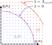
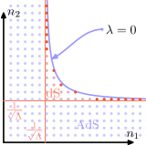
Figure 1: Left panel: Example of a $J=2$ BP landscape, showing the null-$\lambda$ curve separating dS from AdS states, some random low-$\lambda$ states (red) and the cutoff curve. Right panel: a $J=2$ MS-EM landscape, showing the null-$\lambda$ curve separating dS and AdS states (shown superimposed as they are different solutions of (4)), its asymptotes, some random low-$\lambda$ states and state chains (red).

Chained states are arranged by decreasing $\lambda$, and the states with lowest $\lambda$ are always stable. They contribute to the effective cosmological constant distribution in peaks, which become very sharp when $\frac{1}{\sqrt{\Lambda}}$ approaches an integer from below. Thus, the $\lambda$ distribution has a dominant peak coming from the longest state chains, and subdominant peaks separated by a gap from the dominant one which merge with a bulk distribution having an almost constant average behavior before vanishing after reaching the maximum $\lambda$ value of stable dS states, which is $\lambda_{\mathrm{max}}=\frac{2\Lambda}{J(J+3)}$. Figure 2 summarizes the very different behavior of both distributions.

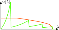
Figure 2: Effective cosmological constant distribution of a $J=2$ BP landscape (flat curve), and a $J=2$ MS-EM landscape (jagged curve).

Therefore, the special form of the null-$\lambda$ hypersurface (8) leads to state chains, which generate peaks in the low-$\lambda$ region of the $\lambda$ distribution, thereby providing an alternative mechanism for finding small values of the effective cosmological constant besides the random closeness, which is also present.

III Anthropic states in the MS-EM landscape

We can look for a set of integers $\{n_{1},\cdots,n_{J}\}$ which approximately solve equation (8), expecting that reasonably good choices will yield very low values of the 1+1 cosmological constant $\lambda$. Choosing the best integer step by step we arrive at the following recurrence relation:

$$\Lambda_{j+1}=f(\Lambda_{j})=\Lambda_{j}-\left\lceil\Lambda_{j}^{-\frac{1}{2}}\right\rceil^{-2}\,,\quad n_{j}=\left\lceil\Lambda_{j}^{-\frac{1}{2}}\right\rceil\,.$$ (9)

The initial value triggering the recurrence is $\Lambda_{1}=\Lambda$. After $J$ steps, we obtain a solution choosing the last integer as $n_{J}=\bigl{\lfloor}\Lambda_{J}^{-1/2}\bigr{\rfloor}$. Equation (9) is a fixed point iteration with superlinear convergence rate, whose solution is thus a double exponential $\Lambda_{j}\approx 2^{\sum^{j-2}_{k=0}(\frac{3}{2})^{k}}\Lambda^{(\frac{3}{2})^{j-1}},\ {}(j\geq 2)$. It can be shown Asensio and Segui (2012) that the resulting fast-growing integers $\{n_{j}\}$ form a node which has always a well-defined stable state on it. Moreover, this node is the end of a very long state chain, which translates in a very narrow peak in the $\lambda$ distribution containing $\sim n_{J}$ states whose support is the interval $[0,\Lambda_{J}/2]$. Thus, we can find the whole peak inside the anthropic range $0\leq\lambda\leq\lambda_{\mathrm{A}}$ for a given $\Lambda$ by equating $\lambda_{\mathrm{A}}=\Lambda_{J}/2$ and solving for $J$, resulting in $J=1+\log_{\frac{3}{2}}\Bigl{(}\frac{\log(\lambda_{\mathrm{A}}/2)}{\log(4\Lambda)}\Bigr{)}$. As an example, with $\lambda_{\mathrm{A}}=10^{-120}$, we can obtain an anthropic peak using $\Lambda=0.1$ and $J=15$, yielding $\sim 10^{57}$ states. Using $\Lambda=0.0002$ and $J=10$ we obtain $10^{59}$ anthropic states with the same $\lambda_{\mathrm{A}}$. We can see that the MS-EM landscape contains a huge amount of anthropic states with moderate values of $J$ for any $\Lambda$, and thus no fine-tuning is needed.

It can be seen that states in the anthropic chains just described are non-generic despite being very numerous. Nevertheless, the peak in the prior distribution can be made very narrow when compared with the full anthropic range, and thus the anthropic factor influencing the cosmological constant prediction can be considered as almost constant. As emphasized in Schwartz-Perlov and Vilenkin (2006), the form of the prior distribution can completely change the prediction, and the narrow peak provided by anthropic chains is an example where the prior can dominate the prediction of the cosmological constant’s value.

IV Conclusions

Trying to reconcile the BP landscape with the KKLT stabilization mechanism leads to the $\alpha^{*}$-problem of the BP model. Addressing this problem requires a model where an exact solution of stable dS and AdS states can be found, and a very simple example of this model is given by the MS-EM landscape. Looking at the states found in this model, we can extrapolate that the assumed fixing of the moduli in the BP case might not be enough to guarantee the existence and stability of the states in all nodes. Thus, we should conclude that such an analysis would dramatically change the conclusions of all counting problems in the BP landscape, in particular the predictions concerning the number of anthropic states.

Moreover, the non-trivial geometrical features of the null-$\lambda$ hypersurface of the MS-EM landscape lead to the existence of state chains, which provide a new mechanism for finding low-$\lambda$ states. This would largely affect all probability computations in this context, as reflected by the existence of a huge number of anthropic states in the model. This non-trivial geometrical fact, with such profound implications in the predictions of the theory, may also well be present, maybe under different forms, in the true string theory landscape.