CERN-PH-TH/2012-202 Flavor Beyond the Standard Universe

Abstract

We explore the possibility that the observed pattern of quark masses is the consequence of a statistical distribution of Yukawa couplings within the multiverse. We employ the anthropic condition that only two ultra light quarks exist, justifying the observed richness of organic chemistry. Moreover, the mass of the recently discovered Higgs boson suggests that the top Yukawa coupling lies near the critical condition where the electroweak vacuum becomes unstable, leading to a new kind of flavor puzzle and to a new anthropic condition. We scan Yukawa couplings according to distributions motivated by high-scale flavor dynamics and find cases in which our pattern of quark masses has a plausible probability within the multiverse. Finally we show that, under some assumptions, these distributions can significantly ameliorate the runaway behavior leading to weakless universes.

1 Introduction

The discovery of the Higgs boson sheds light on the origin of electroweak (EW) symmetry breaking but leaves open the problem of why the weak force is so much stronger than the gravitational force. Despite the enormous experimental and theoretical effort we are still in the dark. We currently have no indications for dynamics beyond the Standard Model (SM) and this raises the question of whether the weak scale is dynamically stabilized in nature or not. At present we cannot discard the possibility that the EW breaking sector is unnatural as a result of environmental selection effects [1]. The common wisdom is that, due to the vast landscape of configurations that are local energy minima, string theory does not uniquely predict the spectrum of particles and interactions as observed in our universe [2]. Eternal inflation might then generate an enormous number of causally-disconnected “pocket universes,” each with its own laws of physics [3].

While the LHC searches are still ongoing, it is too early to draw conclusions regarding the naturalness or unnaturalness of the EW breaking sector. The only new piece of data at our disposal is the mass of the Higgs boson, which has been found to be about 125–126 GeV [4]. It is interesting that the preferred Higgs mass and the top Yukawa are close to their critical values for vacuum stability [5]. This criticality may just be a mere coincidence, but it is also possible that the special value of the top Yukawa is the result of some underlying statistics that pushes the coupling towards an environmental boundary.

The identification of environmental boundaries for quarks is a highly non-trivial task from the following two main reasons. The first is technical in nature: it involves controlling the way masses, forces, and other physical observables vary when couplings are scanned. This typically requires mastering non-perturbative phenomena as well as complicated sets of coupled equations. The second is more fundamental and is due to the fact that, even if we are able to fully control the response to variations in the fundamental laws of nature, one needs to identify the conditions for which hospitable universes can exist. Below we shall not attempt to fully address these two challenges. Instead we shall use a more minimal and weak criterion where we identify an environmental boundary with the condition that the structure of matter and chemistry are not drastically different with respect to our universe. The analysis of Jenkins et al. [6] showed that organic chemistry similar to the one of our own universe generically requires the presence of exactly two ultra light quarks, with masses well below $\Lambda_{\rm QCD}$. We can view vacuum stability as a new anthropic condition. Assuming a single heavy flavor and a fixed Higgs mass of $125\,$GeV, vacuum metastability requires the corresponding Yukawa to be below roughly $y_{t}\leq 1.03$ (or $m_{t}\leq 179\,$GeV). The observed spectrum and the above anthropic boundaries are illustrated in Fig. 1.

Figure 1: The distributions of quark masses and the anthropic boundaries.

It is interesting to note that the distribution of masses shows a pattern, beyond just being hierarchical, in the sense that the four heavier quarks are distributed close to the boundaries, namely, $s,c,b$ are close to the “organic chemistry” boundary, while the top is close the the electroweak instability boundary. No states are found in the “limbo” related to an intermediate mass range. The LHC result on the Higgs mass is an important input because it suggests that the top Yukawa lies close to a catastrophic situation. This criticality can be considered as related to a new problem, the top anthropic flavor puzzle.

In this paper, we will address the question of whether the observed flavor structure can be understood in terms of parameter scanning with anthropic conditions. For simplicity, we will focus only on the hierarchies in the spectrum of quarks. The pattern of CKM mixing angles can be understood as a consequence of such hierarchies in masses, and we will not discuss it here. Similarly, we will not address the issue of lepton masses, although some of our considerations about quarks can be extended to the charged lepton sector as well. Our goal is not to explain the fine details of the quark mass spectrum, but rather to investigate possible mechanisms that explain its general structure. We will show that statistical interpretations of the mass spectrum can exist. Namely, if the distribution of Yukawa couplings in the multiverse is such that it rises towards both boundaries (corresponding to the directions of the two arrows in Fig. 1) then the observed pattern can be explained. Note that in some sense this is more challenging than explaining the cosmological constant, as in that case one requires a monotonic distribution that peaks towards larger values. In the case presented by us (and illustrated in Fig. 1) a two-peak distribution is required. Motivated by the observed flavor hierarchies we shall consider ansätze for the Yukawa couplings that capture the current wisdom regarding generating hierarchies. We discuss various effects that generate not only preference towards small Yukawa but also lead to a second peak of the distribution for large Yukawa.

So far we have discussed distributions in Yukawa couplings, but did not consider the implications of scanning over the Higgs VEV and the Higgs mass. In principle, one can argue that the parameters of the Higgs potential are related to electroweak dynamics and the question of their origin is completely orthogonal to the discussion related to the nature of the observed flavor sector. Thus in the main part of this work we shall just hold the the Higgs parameters (quartic coupling and VEV) to their current values. However, there is an important reasons to go beyond this assumption (see also [7]). In cases where the Yukawa hierarchies are generated by dynamics (say at the Planck scale), one generically expects a runaway behavior towards universes with large Higgs VEV and very small Yukawas [8]. Such possibility, called “the weakless universe” [9], is perfectly viable from an anthropic point of view. We will show that, under certain assumptions, the same toy example that accounts for the observed quark mass spectrum can also greatly ameliorate or even eliminate the runaway behavior towards the weakless universe.

2 Flavor Dynamics

Various mechanisms that address the flavor puzzle have been studied in the literature [10, 11, 12, 13], yet all of them can be summarized by a simple formula for the effective Yukawa couplings $y$:

$$y\propto\epsilon^{Q}\,,$$ (1)

where $\epsilon$ is some small parameter and $Q$ is a flavor-dependent charge. We assume that flavor dynamics occur at some high energy scale.

We can broadly distinguish between two classes, which have similar parametric dependence but lead to very different behavior. (i) The first class includes Froggatt-Nielsen models with horizontal U(1) [10], as well as split fermions in flat extra dimensions [13, 14]. For Froggatt-Nielsen, the parameter $\epsilon$ is matched to the ratio between the flavon VEV and the fundamental scale and $Q$ to the absolute value of the corresponding charge. For split fermions $\epsilon$ can be identified roughly with $\exp(-R/d)^{n}$ ($R$ being the extra dimension size and $d$ the width of the fermion wave function, with $n=1,2$ for a constant or linear bulk mass respectively). The parameter $Q$ corresponds to $(\Delta x_{5}/R)^{n}$, where $\Delta x_{5}$ is the separation between the fermion localization along the extra dimension, $x_{5}$. Within this class of models, $Q$ can only take non-negative values. (ii) The second class includes models with strong dynamics or models within the warped extra dimension framework, where $\epsilon$ can be identified roughly with $(\Lambda_{\rm IR}/\Lambda_{\rm UV})$ and $Q$ is the anomalous dimension [12, 15, 16]. The peculiarity of this class is that $Q$ can be both positive and negative. To distinguish between the two cases we use a different convention for the exponent of this class, and we denote it by $\gamma$.

Starting from class (i), we assume that the parameters $Q$ and $\epsilon$ scan over different vacua within the multiverse. Here we assume that their probability distribution functions (PDF) can be described by general power laws

$$p_{Q}(Q)\propto Q^{n}\,,\qquad p_{\epsilon}(\epsilon)\propto\epsilon^{m}\,,$$ (2)

where $Q\in\left[0,Q_{\rm max}\right]$ and $\epsilon\in\left[0,1\right]$. Since this mechanism is used to explain the existence of light quarks, we consider $p_{Q}(Q)$ favoring larger $Q$ values, hence $n>0$. The resulting Yukawa PDF for $y\in\left[0,y_{0}\right]$ is calculated by performing the integral:

$$p^{\rm(i)}_{y}(y)=\int_{0}^{Q_{\rm max}}dQ\int_{0}^{1}d\epsilon\,\,p_{Q}(Q)\,p_{\epsilon}(\epsilon)\,\delta\left(y-y_{0}\epsilon^{Q}\right)\,,$$ (3)

which leads to

$$p^{\rm(i)}_{y}(y)\propto\frac{1}{y}E_{1+n}\left[-\frac{1+m}{Q_{\rm max}}\log(y/y_{0})\right]\,,$$ (4)

with $m>-1$ and $E_{\nu}(x)$ being the exponential integral function, and where the normalization is yet to be fixed. Note that $Q_{\rm max}$ and $m$ appear together in the form $(1+m)/Q_{\rm max}\,$, so that in practice they are not independent parameters, and we set $m=2$. A natural choice for $y_{0}$ would be the maximal perturbative value of $4\pi$.

An interesting limit is obtained by taking $Q_{\rm max}$ to be very large (yet not strictly $Q_{\rm max}\to\infty$). For a positive $n$ in Eq. (2), this means that $Q$ would be mostly concentrated close to $Q_{\rm max}\,$. We can thus approximate this limit by plugging $\delta(Q-Q_{\rm max})$ into the calculation of $p^{\rm(i)}_{y}(y)$, which gives

$$p^{\rm(i)}_{y}(y)\rightarrow\left(\frac{y}{y_{0}}\right)^{\frac{1+m}{Q_{\rm max}}-1}\sim\frac{1}{y}\,.$$ (5)

Consequently, the rather complicated function in Eq. (4) behaves asymptotically as a simple scale-invariant distribution.

Next we discuss the second class of flavor models, where $y=y_{0}\epsilon^{\gamma}$ and now the exponent $\gamma$ (replacing $Q$) can take also negative values. This allows us to obtain heavy quarks with $y>y_{0}\,$, which means that $y_{0}$ should be taken smaller than $4\pi$. This class can lead to a richer structure of Yukawa distributions. If we adopt a power law distribution for $\gamma$ as in Eq. (2) for $Q$, we will get a PDF for the Yukawa similar to that in Eq. (4), but with an absolute value on the argument of the exponential integral function, which is still a monotonically decreasing function of the UV Yukawa. However, going back one step and fixing $\epsilon$, the behavior of the resulting PDF changes significantly, as a sharp minimum appears at $y=y_{0}\,$. In this case the function can lead to statistical “pressure” towards both small and large Yukawa couplings. This can be understood by noting that the PDF coming from the distribution of $\gamma$ only is $\sim\log^{n}(y/y_{0})/y$, leading to this minimum. An additional piece $\log^{-n-1}\epsilon$ appears when $\epsilon$ is also integrated over. This creates a strong preference towards $\epsilon=1$, which enhances the probability to have $y\simeq y_{0}$ thus washing away the minimum. The minimum is not washed away when the PDF for $\epsilon$ peaks strongly away from unity, for example when there is preference towards small values, e.g. $p_{\epsilon}(\epsilon)\sim\exp(-\alpha\,\epsilon)$ with a large enough $\alpha$.

In practice, for class (ii) models we choose a distribution for $\gamma$ which favors large (positive or negative) values much more pronouncedly than the power law PDF, and thus leads to either light or heavy quarks:

$$p_{\gamma}(\gamma)\propto e^{a\gamma^{2}}\,,$$ (6)

with $a>0$. For simplicity, we keep $\epsilon$ fixed in this case. The resulting (not normalized) Yukawa distribution is

$$p^{\rm(ii)}_{y}(y)\propto\frac{1}{y}\exp\left[a\left(\frac{\log\left(y/y_{0}\right)}{\log\epsilon}\right)^{2}\right]\,.$$ (7)

In the left panel of Fig. 2 we show the two distributions of Eqs. (4) (with $n=m=2$ and $Q_{\rm max}=100$) and (7) (with $a=3.1$, $y_{0}=6.8\times 10^{-3}$ and $\epsilon=0.012$). When $\gamma$ is scanned above roughly 1 there is no sensitivity to the range in which it is varied.

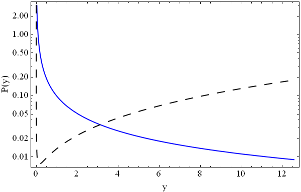
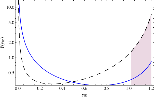
Figure 2: PDF of a single Yukawa coupling. The solid blue and dashed black lines correspond, respectively, to the distributions of $p_{y}^{\rm(i)}$ (Eq. (4) with $n=m=2$ and $Q_{\rm max}=100$) and $p_{y}^{\rm(ii)}$ (Eq. (7) with $a=3.1$, $y_{0}=6.8\times 10^{-3}$ and $\epsilon=0.012$). Left panel: the original distributions as applied at the Planck scale. Right panel: the distributions after one-loop RGE running down to the weak scale. The shaded region is excluded by the requirement of vacuum metastability.

3 Renormalization Group Effects and the Stability Bound

We discuss here how inclusion of the running of Yukawa couplings from the high flavor mediation scale, $\mu_{\mathrm{U}V}$, to the electroweak one, tend to favor heavy quarks. This can be understood because of the presence of a pseudo fixed point at low scale $\mu_{\mathrm{I}R}$. Another aspect that affects the range of possible Yukawa eigenvalues is the requirement that the Higgs potential is not unstable. In this section we consider the effects of the renormalization group equations (RGE) and the stability bound on the Yukawa distribution of a single quark (the case of several flavors is discussed in the following).

Taking an initial value for the top Yukawa coupling in the range $[0,4\pi]$ at the Planck scale, its IR value at the weak scale is presented in Fig. 3, using one-loop RGE. It is evident that for any initial value above $\sim$2 at the Planck scale, the IR Yukawa is 1.3. This can be described analytically:

$$y_{\mathrm{I}R}=\alpha\left(\beta+y_{\mathrm{U}V}^{-2}\right)^{-1/2}\,,$$ (8)

$$\alpha(\mu_{\mathrm{I}R}) = \left[\frac{g_{3}(\mu_{\mathrm{I}R})}{g_{3}(\mu_{\mathrm{U}V})}\right]^{8/7}\left[\frac{g_{2}(\mu_{\mathrm{I}R})}{g_{2}(\mu_{\mathrm{U}V})}\right]^{27/38}\left[\frac{g_{1}(\mu_{\mathrm{I}R})}{g_{1}(\mu_{\mathrm{U}V})}\right]^{-17/82}\,,$$ (9)

$$\beta = \frac{9}{16\pi^{2}}\int_{\mu_{\mathrm{I}R}}^{\mu_{\mathrm{U}V}}\frac{d\mu}{\mu}~{}\alpha^{2}(\mu)~{},$$ (10)

where $g_{1,2,3}$ are the gauge couplings. Since $\beta>1$, the IR Yukawa quickly reaches an asymptotic value $y_{\mathrm{I}R}=\alpha/\sqrt{\beta}$ for large $y_{\mathrm{U}V}\,$, as evident in Fig. 3. For $\mu_{\mathrm{U}V}$ equal to the Planck mass, we find $\alpha=3.6$ and $\beta=7.7$.

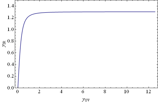
Figure 3: The top Yukawa coupling at the weak scale as a function of the initial value at the Planck scale, after one-loop RGE running.

If we now apply the RGE result of Eq. (8) to the Yukawa distributions in Eqs. (4) and (7) for the initial UV value, we can derive a PDF for the IR value:

$$\begin{split}p^{\rm(i)}_{y}(y_{\mathrm{I}R})&\propto\frac{\alpha^{2}}{y_{\mathrm{I}R}\left(y_{\mathrm{I}R}^{2}\beta^{2}-\alpha^{2}\right)}E_{1+n}\left[-\frac{1+m}{Q_{\rm max}}\log\left(\frac{y_{\mathrm{I}R}/y_{0}}{\sqrt{\alpha^{2}-y_{\mathrm{I}R}^{2}\beta^{2}}}\right)\right]\,,\\ p^{\rm(ii)}_{y}(y_{\mathrm{I}R})&\propto\frac{\alpha^{2}}{y_{\mathrm{I}R}\left(y_{\mathrm{I}R}^{2}\beta^{2}-\alpha^{2}\right)}\exp\left[a\log^{2}\left(\frac{y_{\mathrm{I}R}/y_{0}}{\sqrt{\alpha^{2}-y_{\mathrm{I}R}^{2}\beta^{2}}}\right)/\log^{2}\epsilon\right]\,.\end{split}$$ (11)

These are shown on the right hand side of Fig. 2. Interestingly, the IR Yukawa assumes a binary-like distribution, in which either small or large values are favored, while intermediate values are not.

The stability of the Higgs potential has been thoroughly studied in the literature (see e.g. [5, 17, 18, 19]). The top Yukawa drives the Higgs quartic towards small values and as a result the vacuum becomes unstable or at least metastable in a significant part of the parameter space described by the top and Higgs masses and the strong coupling. The stability and metastability bounds for the top Yukawa are given by [5]

$$y_{t}<0.98+0.0029\left(\frac{m_{h}-125.5\,{\rm GeV}}{1\,{\rm GeV}}\right)+0.0014\left(\frac{\alpha_{s}(m_{Z})-0.1184}{0.0007}\right)\pm 0.0029\,,$$ (12)

$$y_{t}<1.02+0.0018\left(\frac{m_{h}-125.5\,{\rm GeV}}{1\,{\rm GeV}}\right)+0.0017\left(\frac{\alpha_{s}(m_{Z})-0.1184}{0.0007}\right)\pm 0.0055\,,$$ (13)

respectively. Assuming no new physics up to the Planck scale, the conclusion is that present measurements favor the possibility that our electroweak vacuum is metastable. It is quite remarkable to note that for a fixed $125$ GeV Higgs mass the top Yukawa is less than $3\%$ from making our electroweak vacuum unstable! Below we use the requirement of metastability of the Higgs potential as an anthropic upper bound on quark masses.

4 Multi-Flavor Analysis and The Quark Spectrum

We now combine the ingredients above and study the resulting quark mass structure within a multiverse framework. The analysis is based on the following assumptions:

• There is no new physics beyond the SM up to the Planck scale. (As a sensitivity check, we have also analyzed lower UV scales; as long as the flavor mediation scale is large enough, the qualitative behavior described below is unchanged.)

• The Yukawa distributions of Eqs. (4) and (7) are therefore applied at the Planck scale, so that the associated flavor dynamics takes place at that scale or above. Alternatively, we examine also the case where the Yukawa distribution applies at the weak scale, and the RGE play no role.

• The existence of the lightest two (and only two) quarks is ensured by anthropic arguments.

• Only the Yukawa sector of the SM is being scanned over the multiverse, while the gauge and Higgs parameters (quartic coupling and bilinear term) are held fixed. The implications of scanning over the Higgs mass are discussed below in section 5.

The Yukawa couplings of the four heaviest quarks are generated (uncorrelated) at the Planck scale, and then evolved down to the weak scale (equal to the Z mass) using one-loop RGE. In order to represent the quark mass pattern, or more precisely the large difference between the heavy top quark and the light strange, charm and bottom quarks, we define two mass regions: “light” quarks for which the weak scale Yukawa eigenvalues reside in the range corresponding to roughly 60 MeV up to 10 GeV, and “heavy” quarks above 90 GeV (Yukawa coupling greater than 1/2), all evaluated at the Z mass.

On top of the above, we consider the effect of the metastability bound as another anthropic requirement on the quark mass distribution. Note that we cannot simply use Eq. (13) above, since it only applies for one heavy quark. Instead, we use the (simplified) condition [18, 19, 20]

$$\lambda(M_{\rm Pl})>-0.095\,,$$ (14)

where $\lambda$ is the Higgs quartic coupling. In principle, this should be taken to hold for any $\mu$ between the weak scale and the Planck scale, and indeed there is always a minimum of $\lambda(\mu)$ at a scale lower than $M_{\rm Pl}\,$. However, in our numerical calculations we have verified that if we evaluate $\lambda$ only at the Planck scale, the result is hardly affected compared to using the real minimum.

In order to put the numerical results below in proper perspective, we can assume that there is no correlation between the PDF for the various quarks, and that the total PDF is simply the product of the independent individual distributions. In such a case, it is easy to verify that the optimal single quark PDF for explaining the observed spectrum with three light and one heavy quark should be such that

$$P_{\rm light}=75\%\,,\ \,P_{\rm heavy}=25\%\,,$$ (15)

and obviously nothing in the region between the two ranges. Consequently, the probabilities to obtain 3 light quarks and one heavy quark ($P_{\rm 3l|1h}$), 4 light quarks ($P_{\rm 4l}$), and all other cases ($P_{\rm other}$) are

$$P_{\rm 3l|1h}=42\%\,,\ \,P_{\rm 4l}\simeq 32\%\,,\ \,P_{\rm other}\simeq 26\%\,.$$ (16)

We should point out that both the RGE effect as well as the metastability bound induce correlations between multi-quark PDFs, and thus the above result should be only viewed as an approximation for the correct result. However, Eq. (16) can be used as a point of reference for comparison to the results below.

We first compute the probabilities for a single light or heavy quark with the PDFs under consideration, taking into account the RGE from the Planck scale and the metastability bound. These are normalized to the probability for a quark above 60 MeV (as evaluated at the Z mass) and below the metastability bound. The results are:

$$P_{\rm light}^{\rm(i)}=56\%\,,\ \ P_{\rm heavy}^{\rm(i)}=14\%\,,\qquad P_{\rm light}^{\rm(ii)}=58\%\,,\ \ P_{\rm heavy}^{\rm(ii)}=26\%\,,$$ (17)

where we used $n=m=2$ and $Q_{\rm max}=100$ for the class (i) distribution of Eq. (4) and $a=3.1$, $y_{0}=6.8\times 10^{-3}$ and $\epsilon=0.012$ for the class (ii) distribution of Eq. (7). Interestingly, these numbers are not very far from the optimal assignment of Eq. (15). As expected, the numbers for class (ii) are closer to the ideal distribution (especially for $P_{\rm heavy}$), as a result of the two-peak distribution. Furthermore, as we discuss more extensively below, it pushes the Yukawa close to either the small or large anthropic boundaries, consistently with the observed spectrum. In particular, this mechanism can account for the new top anthropic flavor puzzle.

Next, we perform the following exercise. We scan over UV Yukawa distributions and compute the probabilities to have various combinations of light and heavy quarks. The normalization is as before, which means that we account for the “chemistry” requirement in such a way that the full set of anthropically allowed universes corresponds to a probability of 100%. We first consider the class (i) distribution of UV Yukawa couplings given by Eq. (4) for $n=m=2$ and taken as a function of $Q_{\rm max}\,$. The results are presented in Table 1. We verified that the results do not depend strongly on $n$ nor on the actual UV scale (that is, if it is much lower than the Planck scale). Similarly, the results for the class (ii) distribution of Eq. (7) using the parameters $a=3.1$, $y_{0}=6.8\times 10^{-3}$ and $\epsilon=0.012$ are also given in Table 1. In this case, lowering the UV scale does have some effect on the results below (for instance, the probability to have one heavy quark and three light ones goes down from 18% to 9% for a UV scale of $10^{10}$ GeV).

		class (i), Eq.  (4)			class (ii), Eq.  (7)
Probability for		$Q_{\rm max}=10$	$Q_{\rm max}=100$	No RGE	RGE	No RGE
0 heavy, 4 light	without	0	2.4 %	3.2 %	0	0
	with	0.44 %	9.7 %	–	14 %	–
1 heavy, 3 light	without	0.40 %	13 %	11 %	0	0
	with	2.6 %	9.8 %	–	18 %	–
2 heavy, 2 light	without	6.3 %	15 %	14 %	0	0
	with	3.8 %	2.8 %	–	9.4 %	–
3 heavy, 1 light	without	15 %	4.4 %	8.2 %	1.0 %	0.92 %
	with	1.8 %	0.27 %	–	2.2 %	–
4 heavy, 0 light	without	8.3 %	0.35 %	1.8 %	72 %	97 %
	with	0.21 %	0	–	0.21 %	–
2 or more intermediate	without	29 %	24 %	20 %	1.4 %	0
	with	61 %	39 %	–	17 %	–

Table 1: Probabilities of different combinations of heavy and light quarks for class (i) and (ii) distributions without and with the metastability bound (probabilities smaller than 0.1% were rounded down to zero). For class (i) we use $n=m=2$ while for class (ii) $a=3.1$, $y_{0}=6.8\times 10^{-3}$ and $\epsilon=0.012$. The No RGE columns stand for the case without RGE, applying the Yukawa distributions at the weak scale (without the metastability bound) and using $Q_{\rm max}=100$ for class (i).

From the results presented in the table we can draw the conclusion that the observed spectrum with one heavy and three light quarks is plausible in the context of a multiverse in which Yukawa couplings scan. The RGE have two effects: (i) increasing the plausibility to have large Yukawa values, as can be seen from Fig. 2, Eq. (8) and below; (ii) decreasing the probability to have several heavy quarks due to correlations among them. Specifically, the running of a Yukawa coupling in the presence of additional heavy flavors pushes it towards smaller values in the IR. The metastability constraint plays a crucial role in further reducing the plausibility of cases with several heavy quarks, especially for the class (ii) models, where the preference for large Yukawas is much stronger (see Fig. 2). This also means that for class (i), the mass of the top quark is distributed quite uniformly in the region defined as heavy (that is, above 90 GeV), and we find no explanation for the top Yukawa anthropic puzzle, i.e. why $y_{t}$ is just a few percents below the boundary. On the other hand, for class (ii) the probability to obtain a single heavy quark with Yukawa in the range $0.75-1$ is twice as large than the probability to obtain a heavy quark with Yukawa in the range $0.5-0.75$, which constitutes a better explanation for the above puzzle.

To conclude, we find that, for favorable parameters of the different distributions, universes with a quark pattern similar to the one we observe can have probabilities in the range 10-20%. This has to be compared with the reference case of Eq. (16), which gives $P_{\rm 3l|1h}=42\%$.

5 Amelioration of the Runaway Behavior

In [8] it was shown that applying a simple Yukawa distribution as in Eqs. (1) and (2) and using the anthropic requirement for two light quarks makes habitable universes without weak interaction to be far more plausible than ours. This comes from the fact that these distributions allow for arbitrarily low Yukawa values and this is statistically favored since a quadratic PDF for the Higgs VEV, $p_{v}(v)\sim v^{2}/M_{\rm Pl}^{2}\,$, prefers large values of $v$.

This runaway behavior can be cured in models where $y=y_{0}e^{\gamma}$, with $\gamma$ scanning according to Eq. (6), by imposing the following two ad-hoc rules. (i) There is a lower cutoff on the Yukawa, $y_{\mathrm{min}}$. Notice that unlike the analysis in [21], where $y_{\mathrm{min}}$ is of the order of the electron Yukawa, here we use $y_{\mathrm{min}}\ll y_{e}\,$, such that the precise value of $y_{\mathrm{min}}$ has no anthropic significance (see also [22]). (ii) $y_{0}$ scales inversely with the Higgs VEV, such that the part of the distribution responsible for light quarks always falls close to the upper anthropic bound on the two light quarks (here the term “light” refers to the two lightest quarks required by anthropic arguments). Realizing such a rule from first principles requires a dynamical mechanism that relates $y_{0}$ to $\Lambda_{\rm QCD}/v$.

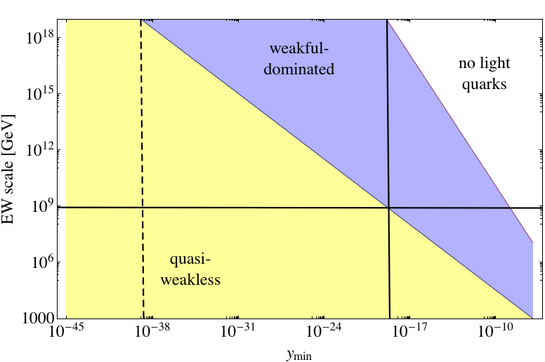
Figure 4: Comparison between the probabilities for the existence of a quark with mass less than $\Lambda_{\rm QCD}$ in a universe with a weak scale similar to ours (“weakful”) and in universes with higher Higgs VEV (“weakless”). The result is shown as a function of the minimum Yukawa coupling $y_{\mathrm{min}}$ and the EW scale $v$. In the yellow shaded region both types of universes have a $\sim 100\%$ probability to produce light quarks, but $R\gg 1$ (defined in Eq. (18)) and thus weakless universes are far more probable. In the blue shaded region we find $R\ll 1$, since the probability for light quarks drops significantly in the weakless universes, making the weakful universe favored. In the white region there are no light quarks in either type of universe.

To illustrate the manner in which this mechanism can cure the runway behavior toward weakless universes, we consider the following probability ratio

$$R=\frac{P\left(m_{\mathrm{light}}\left|v,y_{\mathrm{min}}\right.\right)}{P\left(m_{\mathrm{light}}\left|174\,{\rm GeV},y_{\mathrm{min}}\right.\right)}\times\frac{p_{v}(v)}{p_{v}(174\,{\rm GeV})}\,.$$ (18)

Here $p_{v}(v)\sim v^{2}$ is the PDF for the Higgs VEV and $P(m_{\mathrm{light}}|v,y_{\mathrm{min}})$ is the probability to obtain a quark mass below $\Lambda_{\rm QCD}$, as we scan $\gamma$ according to Eq. (6), for fixed values of the Higgs VEV $v$ and $y_{\mathrm{min}}$. Thus, $R\ll 1$ means that the “weakful” universe (where the weak scale matches our own) is favored over universes with a higher Higgs VEV equal to $v$. By adopting the same values for the parameters as before with the rescaling of $y_{0}$ ($a=3.1$ $\epsilon=0.012$, and $y_{0}=6.8\times 10^{-3}\times 174\,{\rm GeV}/v$), we find that for a rather wide range of $y_{\mathrm{min}}$ the weakful universe is favored, as shown in the blue shaded region of Fig. 4. In particular, for any $y_{\mathrm{min}}>10^{-39}$, the weakless universe with $v=M_{\rm Pl}$ is disfavored (this corresponds to the dashed vertical line in Fig. 4). Furthermore, the required minimal Yukawa values, which ameliorate the runaway behavior, are significantly smaller than the critical Yukawa value $\sim\Lambda_{\rm QCD}/M_{\rm Pl}$, which correspond to the light quark anthropic boundary, as denoted by the solid vertical line of Fig. 4. Note that for $y_{\mathrm{min}}\sim\Lambda_{\rm QCD}/M_{\rm Pl}$ the maximal value for the weak scale is as small as $\sim 10^{9}\,$GeV and the runaway towards the weakless universe is significantly ameliorated. In the white region of Fig. 4 there are no light quarks in either type of universes. The price to pay in using this Yukawa distribution is that the resulting light quarks will tend to be extremely light in general, as dictated by the value of $y_{\mathrm{min}}$.

6 Conclusions

While it has been suggested that the multiverse may explain the cosmological constant and the hierarchy problems, it is generally believed that it cannot be of much use for the flavor puzzle of the SM. The reason is that, while the properties of our universe critically depend on the cosmological constant and the Higgs VEV, many of the flavor parameters – such as the second and third generation masses and mixings – do not seem to affect the properties of ordinary matter. In this paper, we have tried to challenge this point of view.

The starting observation is related to the recent discovery of the Higgs boson. Given the known Higgs mass, a minor modification of the top Yukawa can have dramatic consequences for our universe, triggering an apocalyptic phase transition. So, even if the value of a third-generation quark mass is unrelated to the properties of matter, it can crucially influence the evolution of our universe.

Motivated by this observation, we have studied the possibility that the entire quark mass spectrum is determined by statistical distributions of Yukawa couplings, under the constraint of anthropic conditions. Our assumption is that the SM Yukawa couplings originate from some high-scale flavor dynamics, whose parameters scan within the multiverse.

Our goal is relatively modest. We do not aim at predicting precisely the values of the quark masses and mixings, but we are satisfied with showing that statistics could be the reason behind the observed pattern. The only features of the quark mass spectrum that we want to explain are: (i) two ultra-light quarks ($u$, $d$) with masses much smaller than $\Lambda_{\rm QCD}$; (ii) three quarks ($s$, $c$, $b$) with Yukawas clustered around $\Lambda_{\rm QCD}/M_{W}$, the “chemistry” anthropic boundary; (iii) one heavy quark with Yukawa of order one, at the border of the “stability” anthropic limit.

For Yukawa distributions that are peaked towards small values when evaluated in the UV, RG effects can generate in the IR a second peak for large Yukawa couplings, as a consequence of a pseudo fixed point. However, the values of the Yukawa corresponding to the second peak are excluded by vacuum stability requirements, for a Higgs mass of about 125–126 GeV. As a result, RG effects cannot explain the near-criticality of the top mass, but they help to increase the probability of obtaining some heavy quarks in the spectrum.

Especially interesting is the case of Yukawa distributions emerging from strong dynamics at the high scale. In this case, already in the UV there could be a tendency to populate simultaneously the regions of light and heavy quarks, while disfavoring the intermediate range. We find a plausible probability that an average universe (which satisfies anthropic conditions) has a pattern of quarks similar to what we observe, with one heavy quark at the edge of the stability region.

References

- [1] V. Agrawal, S. M. Barr, J. F. Donoghue and D. Seckel, Phys. Rev. Lett. 80, 1822 (1998) [hep-ph/9801253]; V. Agrawal, S. M. Barr, J. F. Donoghue and D. Seckel, Phys. Rev. D 57, 5480 (1998) [hep-ph/9707380].
- [2] For a review, see M. R. Douglas and S. Kachru, Rev. Mod. Phys. 79, 733 (2007) [arXiv:hep-th/0610102].
- [3] For a review, see A. H. Guth, J. Phys. A 40, 6811 (2007) [arXiv:hep-th/0702178].
- [4] J. Incandela, the CMS collaboration, and F. Gianotti, the ATLAS collaboration, talks given at CERN on July 4, 2012.
- [5] J. Elias-Miro, J. R. Espinosa, G. F. Giudice, G. Isidori, A. Riotto and A. Strumia, arXiv:1112.3022 [hep-ph]; G. Degrassi, S. Di Vita, J. Elias-Miro, J. R. Espinosa, G. F. Giudice, G. Isidori and A. Strumia, arXiv:1205.6497 [hep-ph].
- [6] R. L. Jaffe, A. Jenkins and I. Kimchi, Phys. Rev. D 79, 065014 (2009) [arXiv:0809.1647 [hep-ph]].
- [7] B. Feldstein, L. J. Hall and T. Watari, Phys. Rev. D 74, 095011 (2006) [hep-ph/0608121].
- [8] O. Gedalia, A. Jenkins and G. Perez, Phys. Rev. D 83, 115020 (2011) [arXiv:1010.2626 [hep-ph]].
- [9] R. Harnik, G. D. Kribs and G. Perez, Phys. Rev. D 74, 035006 (2006) [hep-ph/0604027].
- [10] C. D. Froggatt and H. B. Nielsen, Nucl. Phys. B 147, 277 (1979).
- [11] S. Dimopoulos and L. Susskind, Nucl. Phys. B 155, 237 (1979); E. Eichten and K. D. Lane, Phys. Lett. B 90, 125 (1980).
- [12] D. B. Kaplan, Nucl. Phys. B 365, 259 (1991).
- [13] N. Arkani-Hamed and M. Schmaltz, Phys. Rev. D 61, 033005 (2000) [arXiv:hep-ph/9903417].
- [14] D. E. Kaplan and T. M. P. Tait, JHEP 0111, 051 (2001) [hep-ph/0110126].
- [15] A. E. Nelson and M. J. Strassler, JHEP 0009, 030 (2000) [hep-ph/0006251].
- [16] L. Randall and R. Sundrum, Phys. Rev. Lett. 83, 3370 (1999) [hep-ph/9905221]; Y. Grossman and M. Neubert, Phys. Lett. B 474, 361 (2000) [hep-ph/9912408].
- [17] N. Cabibbo, L. Maiani, G. Parisi and R. Petronzio, Nucl. Phys. B 158 (1979) 295; P. Q. Hung, Phys. Rev. Lett. 42 (1979); M. Sher, Phys. Rept. 179 (1989) 273.
- [18] J. A. Casas, J. R. Espinosa and M. Quiros, Phys. Lett. B 342, 171 (1995) [hep-ph/9409458].
- [19] G. Isidori, G. Ridolfi and A. Strumia, Nucl. Phys. B 609, 387 (2001) [hep-ph/0104016].
- [20] S. R. Coleman, Phys. Rev. D 15, 2929 (1977) [Erratum-ibid. D 16, 1248 (1977)].
- [21] J. F. Donoghue, K. Dutta, A. Ross and M. Tegmark, Phys. Rev. D 81, 073003 (2010) [arXiv:0903.1024 [hep-ph]].
- [22] L. J. Hall, M. P. Salem and T. Watari, Phys. Rev. D 76, 093001 (2007) [arXiv:0707.3446 [hep-ph]]; L. J. Hall, M. P. Salem and T. Watari, Phys. Rev. Lett. 100, 141801 (2008) [arXiv:0707.3444 [hep-ph]].