Inference of Extreme Synchrony with an Entropy Measure on a Bipartite Network

Abstract

This article proposes a method to quantify the structure of a bipartite graph using a network entropy per link. The network entropy of a bipartite graph with random links is calculated both numerically and theoretically. As an application of the proposed method to analyze collective behavior, the affairs in which participants quote and trade in the foreign exchange market are quantified. The network entropy per link is found to correspond to the macroeconomic situation. A finite mixture of Gumbel distributions is used to fit the empirical distribution for the minimum values of network entropy per link in each week. The mixture of Gumbel distributions with parameter estimates by segmentation procedure is verified by the Kolmogorov–Smirnov test. The finite mixture of Gumbel distributions that extrapolate the empirical probability of extreme events has explanatory power at a statistically significant level.

I Introduction

The network structure of various kinds of physical and social systems has attracted considerable research attention. A many-body system can be described as a network, and the nature of growing networks has been examined well Albert:02 ; Miura . Power-law properties can be found in the growing networks, which are called complex networks. These properties are related to the growth of elements and preferential attachment Albert:02 .

A network consists of several nodes and links that connect nodes. In the literature on the physics of socio-economic systems Anna , nodes are assumed to represent agents, goods, and computers, while links express the relationships between nodes Milakovic ; Lammer . Network structure is perceived in many cases through the conveyance of information, knowledge, and energy, among others.

In statistical physics, the number of combinations of possible configurations under given energy constraints is related to “entropy.” Entropy is a measure that quantifies the states of thermodynamic systems. In physical systems, entropy naturally increases because of the thermal fluctuations on elements. Boltzmann proposed that entropy $S$ is computed from the possible number of ensembles $g$ by $S=\log g$. For a system that consists of two sub-systems whose respective entropies are $S_{1}$ and $S_{2}$, the total entropy $S$ is calculated as the sum of one of two sub-systems $S_{1}+S_{2}$. This case is attributed to the possible number of ensembles $g_{1}g_{2}$. Entropy in statistical physics is also related to the degree of complexity of a physical system. If the entropy is low (high), then the physical configuration is rarely (often) realized. Energy injection or work in an observed system may be assumed to represent rare situations. Shannon entropy is also used to measure the uncertainty of time series Anna:07 .

The concept of statistical–physical entropy was applied by Bianconi Bianconi to measure network structure. She considered that the complexity of a network is related to the number of possible configurations of nodes and links under some constraints determined by observations. She calculated the network entropy of an arbitrary network in several cases of constraints.

Researchers have used a methodology to characterize network structure with information-theoretic entropy Dehmer:11 ; Wilhelm ; Rashevsky:55 ; Trucco:56 ; Mowshowitz:53 ; Aki . Several graph invariants such as the number of vertices, vertex degree sequence, and extended degree sequences have been used in the construction of entropy-based measures Wilhelm ; Aki .

II An entropy measure on a bipartite network

The number of elements in socio-economic systems is usually very large, and several restrictions or finiteness of observations can be found. Therefore, we need to develop a method to infer or quantify the affairs of the entire network structure from partial observations. Specifically, many affiliation relationships of socio-economic systems can be expressed as a bipartite network. Describing the network structure of complex systems that consist of two types of nodes by using the bipartite network is important. A bipartite graph model also can be used as a general model for complex networks Guillaume:06 ; Holyst:07 ; Tumminello . Tumminello et al. proposed a statistical method to validate the heterogeneity of bipartite networks Tumminello .

Suppose a symmetric binary two-mode network can be constructed by linking $K$ groups (A node) and $M$ participants (B node) if the participants belong to groups. Assume that we can count the number of participants in each group within the time window $[t\delta,(t+1)\delta]\quad(t=1,2,3,\ldots)$, which is defined as $m_{i}(t)\quad(i=1,2,\ldots,K)$.

Let us assume a bipartite graph consisting of $A$ nodes and $B$ nodes, of which the structure at time $t$ is described as an adjacency matrix $C_{ij}(t)$. We also assume that $A$ nodes are observable and $B$ nodes are unobservable. That is, we only know the number of participants ($B$ node) belonging to $A$ nodes $m_{i}(t)$. We do not know the correct number of $B$ nodes, but we assume that it is $M$. In this setting, how do we measure the complexity of the bipartite graph from $m_{i}(t)$ at each observation time $t$?

The network entropy is defined as a logarithmic form of the number of possible configurations of a network under a constraint Bianconi . We can introduce the network entropy at time $t$ as a measure to quantify the complexity of a bipartite network structure. The number of possible configurations under the constraint $m_{i}(t)=\sum_{j=1}^{M}C_{ij}(t)$ may be counted as

$$N(t)=\prod_{i=1}^{K}\left(\begin{array}[]{c}M\\ m_{i}(t)\end{array}\right)=\prod_{i=1}^{K}\frac{M!}{m_{i}(t)!(M-m_{i}(t))!}.$$ (1)

Then, the network entropy is defined as $\Sigma(t)=\ln N(t)$. Inserting Eq. (1) into this definition, we have

$$\Sigma(t)=K\sum_{n=1}^{M}\ln n-\sum_{i=1}^{K}\sum_{n=1}^{M-m_{i}(t)}\ln n-\sum_{i=1}^{K}\sum_{n=1}^{m_{i}(t)}\ln n.$$ (2)

Note that, because $0!=1$, $\sum_{n=1}^{0}\ln n=0$. Obviously, if $m_{i}(t)=M$ for any $i$, then $\Sigma(t)=0$. If $m_{i}(t)=0$ for any $i$, then $\Sigma(t)=0$. The lower number of combinations gives a lower value of $\Sigma(t)$. To eliminate a difference in the number of links, we consider the network entropy per link defined as

$$\sigma[m_{1}(t),\ldots,m_{K}(t)]=\frac{\Sigma(t)}{\sum_{i=1}^{K}m_{i}(t)}.$$ (3)

This quantity shows the degree of complexity of the bipartite network structure. We may capture the temporal development of the network structure from the value of $\sigma(t)$. The network entropy per link $\sigma(t)$ is also an approximation of the ratio of the entropy rate for $m_{i}(t)$ to its mean so that

$$\sigma(t)=\frac{\frac{1}{K}\Sigma[m_{1}(t),\ldots,m_{K}(t)]}{\frac{1}{K}\sum_{i=1}^{K}m_{i}(t)}\approx\frac{\Sigma[{\bf m}(t)]}{\langle m(t)\rangle},$$ (4)

where the entropy rate and the mean are, respectively, defined as

$$\Sigma[{\bf m}(t)] = \lim_{K\rightarrow\infty}\frac{1}{K}\Sigma[m_{1}(t),\ldots,m_{K}(t)],$$ (5)

$$\langle m(t)\rangle = \lim_{K\rightarrow\infty}\frac{1}{K}\sum_{i=1}^{K}m_{i}(t).$$ (6)

The ratio of the entropy rate to the mean tells us the uncertainty of the mean from a different point of view from the coefficient of variation ($C.V.=\mbox{standard deviation}/\mbox{mean}$).

(a) (b)

Figure 1: (a) Plots between $\sigma(t)$ and degree of monopolization $k$. Each curve represents the relation between $\sigma(t)$ and $k$. Filled squares numerical values for $M=1000$, unfilled circles for $M=2000$, filled circles for $M=3000$, and unfilled triangle for $M=4000$. (b) Plots between $\sigma(t)$ and density of links $p$. Each curve represents the relation between $\sigma(t)$ and $k$. Filled squares numerical values for $M=1000$, unfilled circles for $M=2000$, filled circles for $M=3000$, and unfilled triangle for $M=4000$.

To understand the fundamental properties of Eq. (3), we compute $\sigma(t)$ in simple cases. Consider values of entropy for several cases at $K=100$ with different $M$. We assume that the total number of links is fixed at 100, which is the same as the number of $A$ nodes, and we confirm the dependence of $\sigma(t)$ on the degree of monopolization. We assign the same number of links at each $A$ node. That is, we set

$$m_{i}(t)=\left\{\begin{array}[]{ll}100/k&i=1,\ldots,k\\ 0&i=k+1,\ldots,K\end{array}\right.,$$ (7)

where $k$ can be set as 1, 2, 4, 5, 10, 20, 50, or 100. In this case, we can calculate $\sigma(t)$ as follows:

$$\sigma(t) = \frac{\sum_{i=1}^{k}\ln\left(\begin{array}[]{c}M\\ 100/k\end{array}\right)}{\sum_{i=1}^{k}100/k}$$ (10)

$$= \frac{k}{100}\Bigl{(}\ln M!-\ln(100/k)!-\ln(M-100/k)!\Bigr{)}.$$ (11)

Fig. 1 a shows the relationship between $\sigma(t)$ and the degree of monopolization at $M=1,000$, $2,000$, $3,000$, and $4,000$. The network entropy per link $\sigma(t)$ is small if a small population of nodes occupies a large number of links. The multiplication regime gives a large value of $\sigma(t)$. The value of $\sigma(t)$ is a monotonically increasing function in terms of $k$. As $M$ increases, the value of $\sigma(t)$ increases. From this instance, we confirmed that $\sigma(t)$ decreases with the degree of monopolization at $A$ nodes.

Next, we confirm the dependency of $\sigma(t)$ on the density of links. We assume that each element of an adjacency matrix $C_{ij}(t)$ is given by an i.i.d. Bernoulli random variable with a successful probability of $p$. Then, $m_{i}(t)=\sum_{j=1}^{M}C_{ij}(t)$ is sampled from an i.i.d. binomial distribution $Bin(p,M)$. In this case, one can approximate $\sigma(t)$ as

$$\sigma(t) = \frac{\frac{1}{K}\sum_{i=1}^{K}\Sigma[m_{i}(t)]}{\frac{1}{K}\sum_{i=1}^{K}m_{i}(t)}$$ (16)

$$\approx \frac{\langle\Sigma[m_{1}(t)]\rangle}{\langle m_{1}(t)\rangle}$$

$$= \frac{1}{M}\sum_{k=1}^{M}\left(\begin{array}[]{c}M\\ k\end{array}\right)p^{k-1}(1-p)^{M-k}\ln\left(\begin{array}[]{c}M\\ k\end{array}\right)$$

Fig. 1 b shows the plots of $\sigma(t)$ versus $p$ obtained from both Monte Carlo simulation with random links drawn from Bernoulli trials and Eq. (16). The number of links at each $A$ node monotonically increases as $p$ increases. $\sigma(t)$ decreases as the density of links decreases. The dependence of the entropy per link on $p$ is independent of $M$.

III Empirical analysis

The application of network analysis to financial time series has been advancing. Several researchers have investigated the network structure of financial markets Bonanno:03 ; Gworek:09 ; Podnik:09 ; Iori:08 . Bonanno et al. examined the topological characterization of the correlation-based minimum spanning tree (MST) of real data Bonanno:03 . Gworek et al. analyzed the exchange rate returns of 38 currencies (including gold) and computed the characteristic path length and average weighted clustering coefficient of the MST topology of the graph extracted from the cross-correlations for several base currencies Gworek:09 . Podnik et al. Podnik:09 examined the cross-correlations between volume changes and price changes for the New York Stock Exchange, Standard and Poor’s 500 index, and 28 worldwide financial indices. Iori et al. Iori:08 analyzed the network topology of the Italian segment of the European overnight money market and investigated the evolution of these banks’ connectivity structure over the maintenance period. These studies collectively aimed to detect the susceptibility of network structures to macroeconomic situations.

Data collected from the ICAP EBS platform were used. The data period spanned May 28, 2007 to November 30, 2012 ICAP . The data included records for orders (BID/OFFER) and transactions for currencies and precious metals with a one-second resolution. The data set involved 94 currency pairs consisting of 39 currencies, 11 precious metals, and 2 basket currencies (AUD, NZD, USD, CHF, JPY, EUR, CZK, DKK, GBP, HUF, ISK, NOK, PLN, SEK, SKK, ZAR, CAD, HKD, MXC, MXN, MXT, RUB, SGD, XAG, XAU, XPD, XPT, TRY, THB, RON, BKT, ILS, SAU, DLR ,KES, KET, AED, BHD, KWD, SAR, EUQ, USQ, CNH, AUQ, GBQ, KZA, KZT, BAG, BAU, BKQ, LPD, and LPT)

III.1 The total number

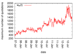
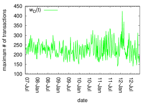
The number of quotations and transactions in each currency pair was extracted from the raw data. Let $m_{X,i}(t)\quad(t=0,\ldots;i=1,\ldots,K)$ be the number of quotations ($X=P$) or transactions ($X=D$) within every minute ($\delta=1$ [min]) for a currency pair $i$ ($K=94$) at time $t$. Let $c_{X}(t)$ be denoted as the total number of quotations ($X=P$) and transactions ($X=D$), which is defined as

$$c_{X}(t)=\sum_{i=1}^{K}m_{X,i}(t).$$ (17)

Let us consider the maximum value of $c_{X}(t)$ in each week:

$$w_{X}(s)=\max_{t\in W(s)}\{c_{X}(t)\},$$ (18)

where $W(s)\quad(s=1,\ldots,T)$ represents a set of times included in the $s$-th week. A total of 288 weeks are included in the data set ($T=288$). Fig. 2 shows the maximum values $c_{X}(t)$ for the period from May 28, 2007 to November 30, 2012.

(a) (b)

Figure 2: (a) The maximum values of the number of quotations within 1 minute in every week. (b) the maximum values of the number of transactions within 1 minute in every week.

According to the extreme value theorem, the probability density for maximum values can be assumed to be a Gumbel density:

$$P(w_{X};\mu_{X},\rho_{X})=\frac{1}{\rho_{X}}\exp\Bigl{(}-\frac{w_{X}-\mu_{X}}{\rho_{X}}-e^{-\frac{w_{X}-\mu_{X}}{\rho_{X}}}\Bigr{)},$$ (19)

where $\mu_{X}$ and $\rho_{X}$ are the location and scale parameters, respectively. Under the assumption of the Gumbel density, these parameters are estimated with the maximum likelihood procedure. The log–likelihood function for $T$ observations $w_{X}(s^{\prime})\quad(s^{\prime}=1,\ldots,T)$ under Eq. (19) is defined as

$$l(\mu_{X},\rho_{X})=\sum_{s^{\prime}=1}^{T}\ln\Bigl{[}\frac{1}{\rho_{X}}\exp\Bigl{(}-\frac{w_{X}(s^{\prime})-\mu_{X}}{\rho_{X}}-e^{-\frac{w_{X}(s^{\prime})-\mu_{X}}{\rho_{X}}}\Bigr{)}\Bigr{]}.$$ (20)

The maximum likelihood estimators are obtained by maximizing the log-likelihood function. Partially differentiating $l(\mu_{X},\rho_{X})$ in terms of $\mu_{X}$ and $\rho_{X}$ and setting them to zero, one has its maximum likelihood estimators as

$$e^{-\frac{\hat{\mu}_{X}}{\hat{\rho}_{X}}} = \frac{1}{T}\sum_{s^{\prime}=1}^{T}e^{-\frac{w_{X}(s^{\prime})}{\hat{\rho}_{X}}},$$ (21)

$$\hat{\rho}_{X} = \frac{1}{T}\sum_{s^{\prime}=1}^{T}w_{X}(s^{\prime})-\frac{\sum_{s^{\prime}=1}^{T}e^{-\frac{w_{X}(s^{\prime})}{\hat{\rho}_{X}}}w_{X}(s^{\prime})}{\sum_{s^{\prime}=1}^{T}e^{-\frac{w_{X}(s^{\prime})}{\hat{\rho}_{X}}}}$$ (22)

Their derivation is shown in Appendix A. The parameters are estimated as $\hat{\mu}_{P}=772.179499$, $\hat{\rho}_{P}=281.741815$, $\hat{\mu}_{D}=206.454884$, and $\hat{\rho}_{D}=35.984804$.

The Kolmogorov–Smirnov (KS) test is conducted to determine the statistical significance of the estimated distributions. The KS test is a popular statistical method of assessing the difference between observations and its assumed distribution by p-value, which is a measure of probability where a difference between the two distributions happens by chance. Large p-values imply that the observations are sampled from the assumed distribution in the null hypothesis with high significance. Let $w_{X}(s)\quad(s=1,\ldots,T)$ be $T$ observations, and let $K_{T}$ be a test statistic

$$K_{T}=\sup_{1\leq s^{\prime}\leq T}\sqrt{T}\Bigl{|}F_{T}(w_{X}(s^{\prime}))-F(w_{X}(s^{\prime}))\Bigr{|},$$

where $0\leq F(v)\leq 1$ is an assumed cumulative distribution in a null hypothesis and $F_{T}(v)$ an empirical one based on $T$ observations such that $F_{T}(v)=k/T$, in which $k$ represents the number of observations satisfying $v_{X}(s)\leq v(s=1,\ldots,T)$. The p-value is computed from the Kolmogorov–Smirnov distribution.

The KS test is conducted under the assumption of the Gumbel distribution for the maximum value corresponding to Eq. (25):

$$F(w_{X};\mu_{X},\rho_{X})=\exp\Bigl{[}-\exp\bigl{(}-\frac{w_{X}-\mu_{X}}{\rho_{X}}\bigr{)}\Bigr{]}.$$ (23)

The p-values of the KS test are shown in Tab. 1. The stationary Gumbel assumption cannot explain the maximum values for quotes with a 5% significance level in the KS test. The stationary Gumbel assumption may not be accepted in the case of the block maximum number of quotes. The dominant reason is the strong nonstationarity of the maximum number of quotes. During the last five years, the currencies and pairs quoted in the electronic brokerage market increased. The mean value of the total number constantly increased. In fact, the maximum number of quotations $w_{P}(t)$ reached the maximum value on 30 July, 2012. The nonstationarity breaks the assumption of the extreme value theorem.

It is confirmed that the stationary Gumbel assumption can be accepted for the block maxima of transactions in each week using the KS test with a 5% significance level. The maximum number of transactions $w_{D}(t)$ was reached on on January 30, 2012. This period seems to be related to the extreme synchrony.

Table 1: The p-values of statistical tests under a stationary assumption of the Gumbel distribution for the maximum values.

p-val (P)	KS-val (P)	p-val (D)	KS-val (D)
0.041374	1.392521	0.586818	0.774087

III.2 Network entropy per link

The proposed method based on statistical–physical entropy is applied to measure the states of the foreign exchange market. The relationship between a bipartite network structure and macroeconomic shocks or crises was investigated, and the occurrence probabilities of extreme synchrony were inferred. We compute a statistical–physical entropy per link from $m_{X,i}(t)(X\in\{P,D\})$ with Eqs. (2) and (3), which are denoted as $\sigma_{X}(t)$. $\sigma_{P}(t)$ and $\sigma_{D}(t)$.

Since small values of $\sigma_{X}(t)$ correspond to a concentration of links at a few nodes or a dense network structure, let us consider the minimum value of $\sigma_{X}(t)$ every week:

$$v_{X}(s)=\min_{t\in W(s)}\{\sigma_{X}(t)\},$$ (24)

where $W(s)\quad(s=1,\ldots,T)$ represents a set of times included in the $s$-th week. A total of 288 weeks are included in the data set ($T=288$). According to the extreme value theorem, the probability density for minimum values can be assumed to be the Gumbel density:

$$P(v_{X};\mu_{X},\rho_{X})=\frac{1}{\rho_{X}}\exp\Bigl{(}\frac{v_{X}+\mu_{X}}{\rho_{X}}-e^{\frac{v_{X}+\mu_{X}}{\rho_{X}}}\Bigr{)},$$ (25)

where $\mu_{X}$ and $\rho_{X}$ are the location and scale parameters, respectively. Under the assumption of the Gumbel density, these parameters are estimated with the maximum likelihood procedure. The log–likelihood function for $T$ observations $v_{X}(s^{\prime})\quad(s^{\prime}=1,\ldots,T)$ under Eq. (25) is defined as

$$l(\mu_{X},\rho_{X})=\sum_{s^{\prime}=1}^{T}\ln\Bigl{[}\frac{1}{\rho_{X}}\exp\Bigl{(}\frac{v_{X}(s^{\prime})+\mu_{X}}{\rho_{X}}-e^{\frac{v_{X}(s^{\prime})+\mu_{X}}{\rho_{X}}}\Bigr{)}\Bigr{]}.$$ (26)

Partially differentiating $l(\mu_{X},\rho_{X})$ in terms of $\mu_{X}$ and $\rho_{X}$ and setting them to zero yields its maximum likelihood estimators as

$$e^{-\frac{\hat{\mu}_{X}}{\hat{\rho}_{X}}} = \frac{1}{T}\sum_{s^{\prime}=1}^{T}e^{\frac{v_{X}(s^{\prime})}{\hat{\rho}_{X}}},$$ (27)

$$\hat{\rho}_{X} = \frac{\sum_{s^{\prime}=1}^{T}e^{\frac{v_{X}(s^{\prime})}{\hat{\rho}_{X}}}v_{X}(s^{\prime})}{\sum_{s^{\prime}=1}^{T}e^{\frac{v_{X}(s^{\prime})}{\hat{\rho}_{X}}}}-\frac{1}{T}\sum_{s^{\prime}=1}^{T}v_{X}(s^{\prime}).$$ (28)

These derivations are shown in Appendix B. The parameter estimates are computed as $\hat{\mu}_{P}=-4.865382$, $\hat{\rho}_{P}=0.110136$, $\hat{\mu}_{D}=-5.010175$, and $\hat{\rho}_{D}=0.120809$ with Eqs. (27) and (28).

The KS test is conducted for the Gumbel distribution for the minimum values corresponding to Eq. (25):

$$F(v_{X};\mu_{X},\rho_{X})=1-\exp\Bigl{[}-\exp\bigl{(}\frac{v_{X}+\mu_{X}}{\rho_{X}}\bigr{)}\Bigr{]}.$$ (29)

The p-value of the distribution is shown in Tab. 2. The stationary Gumbel assumption cannot explain the synchronizations observed in both quotes and transactions completely with a 5% significance level. The stationary Gumbel assumption is rejected because there is a stationary assumption to derive the extreme value distribution. If we can weaken this assumption, then the goodness of fit may be improved.

Table 2: The p-values of statistical tests under a stationary Gumbel assumption.

p-val (P)	KS-val (P)	p-val (D)	KS-val (D)
0.001393	1.906528	0.019241	1.523791

IV Probability of extreme synchrony

The literature detecting structural breaks or change points in an economic time series Goldfeld ; Tobias ; Scalas ; Cheong points out that nonstationary time series are constructed from locally stationary segments sampled from different distributions. Goldfeld and Quandt conducted a pioneering work on the separation of stationary segments Goldfeld . Recently, a hierarchical segmentation procedure was also proposed by Choeng et al. under the Gaussian assumption Cheong . We applied this concept to define the segments for $v_{X}(s^{\prime})\quad(s^{\prime}=1,\ldots,T)$.

Let us consider the null model $L_{1}$, which assumes that all the observations $v_{X}(s^{\prime})\quad(s^{\prime}=1,\ldots,T)$ are sampled from a stationary Gumbel density parameterized as $\mu$ and $\rho$. An alternative model $L_{2}(s)$ assumes that the left observations $v_{X}(s^{\prime})\quad(s^{\prime}=1,\ldots,s)$ are sampled from a stationary Gumbel density parameterized as $\mu_{L}$ and $\rho_{L}$, and that the right observations $v_{X}(s^{\prime})\quad(s^{\prime}=s+1,\ldots,T)$ are sampled from a stationary Gumbel density parameterized as $\mu_{R}$ and $\rho_{R}$.

Denoting likelihood functions as

$$L_{1}(\mu,\rho) = \prod_{s^{\prime}=1}^{T}P(v_{X}(s^{\prime});\mu,\rho),$$ (30)

$$L_{2}(s;\mu_{L},\rho_{L},\mu_{R},\rho_{R}) = \prod_{s^{\prime}=1}^{s}P(v_{X}(s^{\prime});\mu_{L},\rho_{L})$$ (31)

$$\times \prod_{s^{\prime}=s+1}^{T}P(v_{X}(s^{\prime});\mu_{R},\rho_{R}),$$

the difference between the log–likelihood functions can be defined as

$$\Delta(s)=\log L_{2}(s)-\log L_{1}.$$ (32)

$\Delta(s)$ can be approximated as the Shannon entropy $H[p]=-\int_{\infty}^{\infty}\mbox{d}v\log p(v)p(v)$:

$$\Delta(s) \approx TH[P(v_{X};\mu,\rho)]$$

$$- sH[P(v_{X};\mu_{L},\rho_{L})]-(T-s)H[P(v_{X};\mu_{R},\rho_{R})].$$

Since the Shannon entropy of the Gumbel density expressed in Eq. (19) is calculated as

$$H[P(v_{X};\mu_{X},\rho_{X})]=\ln\rho_{X}-\gamma+1,$$ (34)

where $\gamma$ represents Euler’s constant, defined as

$$\gamma=\int_{0}^{\infty}\ln te^{-t}\mbox{d}t,$$ (35)

we obtain

$$\Delta(s)\approx T\ln\rho-s\ln\rho_{L}-(T-s)\ln\rho_{R}.$$ (36)

In the context of model selection, several information criteria are proposed. The information criterion provides both goodness of fit of the model to the data and model complexity. For the sake of simplicity, we use the Akaike information criterion (AIC) to determine the adequate model. The AIC for a model with the number of parameters $K$ and the maximum likelihood of $L$ is defined as

$$AIC=-2\ln L+2K.$$ (37)

We can compute the difference in AIC between model $L_{2}$ and model $L_{1}(s)$ as

$$\Delta_{AIC}(s) = \mbox{AIC of $L_{2}(s)$}-\mbox{AIC of $L_{1}$}$$ (38)

$$\approx -2\bigl{(}T\ln\hat{\rho}-s\ln\hat{\rho}_{L}-(T-s)\ln\hat{\rho}_{R}\bigr{)}+4,$$

$$= -2\Delta(s)+4$$

since the number of parameters of $L_{1}$ is 2, that of $L_{2}(s)$ is 4, and the maximum likelihood is obtained by using their maximum likelihood estimators calculated from

$$\hat{\rho} = \frac{\sum_{s^{\prime}=1}^{T}e^{\frac{v_{X}(s^{\prime})}{\hat{\rho}_{X}}}v_{X}(s^{\prime})}{\sum_{s^{\prime}=1}^{T}e^{\frac{v_{X}(s^{\prime})}{\hat{\rho}_{X}}}}-\frac{1}{T}\sum_{s^{\prime}=1}^{T}v_{X}(s^{\prime})$$ (39)

$$\hat{\rho}_{L} = \frac{\sum_{s^{\prime}=1}^{s}e^{\frac{v_{X}(s^{\prime})}{\hat{\rho}_{L}}}v_{X}(s^{\prime})}{\sum_{s^{\prime}=1}^{s}e^{\frac{v_{X}(s^{\prime})}{\hat{\rho}_{L}}}}-\frac{1}{s}\sum_{s^{\prime}=1}^{s}v_{X}(s^{\prime})$$ (40)

$$\hat{\rho}_{R} = \frac{\sum_{s^{\prime}=s+1}^{T}e^{\frac{v_{X}(s^{\prime})}{\hat{\rho}_{R}}}v_{X}(s^{\prime})}{\sum_{s^{\prime}=s+1}^{T}e^{\frac{v_{X}(s^{\prime})}{\hat{\rho}_{R}}}}-\frac{1}{T-s}\sum_{s^{\prime}=s+1}^{T}v_{X}(s^{\prime})$$

Therefore, $P(v_{X};\mu_{L},\rho_{L})$ is maximally different from $P(v_{X};\mu_{R},\rho_{R})$ when $\Delta(s)$ assumes a maximal value. This spectrum has a maximum at some time $s^{*}$, which is denoted as

$$\Delta^{*}_{AIC}=\Delta_{AIC}(s^{*})=\max_{s}\Delta_{AIC}(s).$$ (42)

The segmentation can be used recursively to separate the time series into further smaller segments. We do this iteratively until all segment boundaries have converged onto their optimal segment, defined by a stopping (termination) condition.

Several termination conditions were discussed in previous studies Cheong . Assuming that $\Delta_{0}>0$, we terminate the iteration if $\Delta_{AIC}^{*}$ is less than a typical conservative threshold of $\Delta_{0}=10$, while the procedure is recursively conducted if $\Delta_{AIC}^{*}$ is larger than $\Delta_{0}$. We checked the robustness of this segmentation procedure for $\Delta_{0}$. $\Delta_{0}$ gives a statistical significance level of termination. The value of $\Delta_{0}$ is related to statistical significance. According to Wilks theorem, $-2\Delta(s)$ follows a chi-squared distribution with a degree of freedom $r$, where $r$ is given by the difference between the number of parameters assumed in the null hypothesis and one in the alternative hypothesis. In this case, $r=2$. Hence, the cumulative distribution function of $\Delta^{*}_{AIC}$ may follow

$$\mbox{Pr}[\Delta^{*}_{AIC}>x]=1-\gamma\Bigl{(}1,\frac{x-4}{2}\Bigr{)}.$$ (43)

Therefore, setting the threshold $\Delta_{0}=10$ implies that the segmentation procedure is tuned as a 4.928% statistical significance level.

Let the number of segments be $L_{X}$, the parameter estimates be $\{\mu_{X,j},\rho_{X,j}\}$ at the $j$-th segment, and the length of the $j$-th segment be $\tau_{X,j}$, where $\sum_{j=1}^{R_{X}}\tau_{X,j}=T$. The cumulative probability distribution for $v_{X}(s)\quad(s=1,\ldots,T)$ may be assumed to be a finite mixture of Gumbel distributions:

$$\mbox{Pr}(V_{X}\leq v_{X}) = \int_{-\infty}^{v_{X}}\sum_{j=1}^{R_{X}}\frac{\tau_{X,j}}{T}P(v_{X}^{\prime};\mu_{X,j},\rho_{X,j})\mbox{d}v_{X}^{\prime}$$ (44)

$$= \sum_{j=1}^{R_{X}}\frac{\tau_{X,j}}{T}\Bigl{\{}1-\exp\bigl{[}-e^{\frac{v_{X}+\mu_{X,j}}{\rho_{X,j}}}\bigr{]}\Bigr{\}},$$

(a) (b)

Figure 3: Temporal development of (a) $v_{P}(s)$ and (b) $v_{D}(s)$ from May 28, 2007 to November 30, 2012.

Tabs. 4 and 4 show parameter estimates of $v_{P}(s)$ and $v_{D}(s)$ using the recursive segmentation procedure.

Table 3: Parameter estimates obtained from the weekly minimum values of network entropy for quotations with the recursive segmentation procedure.

$j$	start date	end date	$\tau/T$	$\hat{\mu}_{X,j}$	$\hat{\rho}_{X,j}$
1	May 28, 2007	Oct. 15, 2007	0.072917	-4.965486	0.078571
2	Oct. 22, 2007	Aug. 17, 2009	0.333333	-4.829061	0.080558
3	Aug. 24, 2009	Oct. 21, 2011	0.274306	-4.880156	0.099532
4	Feb. 28, 2011	Jul. 30, 2012	0.260417	-4.798364	0.058265
5	Aug. 6, 2012	Sep. 10, 2012	0.020833	-4.856415	0.121566
6	Sep. 17, 2012	Nov. 26, 2012	0.038194	-5.031930	0.071871

Table 4: Parameter estimates obtained from the weekly minimum values of network entropy for transactions with the recursive segmentation procedure.

$j$	start date	end date	$\tau/T$	$\hat{\mu}_{X,j}$	$\hat{\rho}_{X,j}$
1	May 28, 2007	Mar. 16, 2009	0.329861	-4.903660	0.072684
2	Mar. 23, 2009	Jun. 14, 2010	0.225694	-4.990569	0.088420
3	Jun. 21, 2010	Dec. 5, 2011	0.267361	-5.065305	0.087721
4	Dec. 12, 2011	Mar. 12, 2012	0.048611	-4.826384	0.174328
5	Mar. 19, 2012	Apr. 30, 2012	0.024306	-5.108679	0.011079
6	May 7, 2012	Nov. 26, 2012	0.104167	-5.131156	0.079630

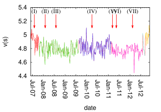
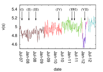
Fig. 3 shows the temporal development of $v_{P}(s)$ and $v_{D}(s)$ from May 28, 2007 to November 30, 2012. $R_{P}=6$ and $R_{D}=6$ are obtained from $v_{X}(s)$ using the proposed segmentation procedure. During the observation period, the global financial system suffered from the following significant macroeconomic shocks and crises: (I) the BNP Paribas shock (August 2007), (II) the Bear Stearns shock (February 2008), (III) the Lehman shock (September 2008 to March 2009), (IV) the European sovereign debt crisis (April to May 2010), (V) the East Japan tsunami (March 2011), (VI) the United States debt-ceiling crisis (May 2011), and (VII) the Bank of Japan’s 10 trillion JPY gift on Valentine’s Day (February 2012).

Before entering these global affairs, both $v_{P}(s)$ and $v_{D}(s)$ took large values. Note that, during the (I) Paribas shock, the (II) Bear Stearns and the (III) Lehman shock $v_{P}(s)$ and $v_{D}(s)$ took smaller values than they did during the previous term. This implies that a global shock may drive many participants and that these participants may trade the same currencies at the same time. The smallest values $v_{P}(s)$ and $v_{D}(t)$ correspond to the days of the (II) Bear Stearns shock, the (III) Lehman shock, and the (VI) Euro crisis. These days are generally related to the start or the end of macroeconomic shocks or crises. The period from December 2011 to March 2012 shows that the values of $v_{D}(s)$ are smaller than they were during other periods. This result implies that, during said period, singular patterns appeared in the transactions.

(a) (b)

Figure 4: Cumulative distribution functions for the minimum values of the entropy per link in each week (a) $v_{P}(s)$ and (b) $v_{D}(s)$. Filled squares represent the empirical distribution of $v_{P}(s)$, and unfilled circles represent the empirical distribution of $v_{D}(s)$. A solid curve represents the estimated distribution of $v_{P}(s)$, and a dashed curve represents the estimated distribution of $v_{D}(s)$.

Fig. 4 shows both the empirical and estimated cumulative distribution functions of $v_{P}(s)$ and $v_{D}(s)$. The estimated cumulative distributions are drawn from Eq. (44) with parameter estimates. The KS test verifies this mixing assumption. The distribution estimated by the finite mixture of Gumbel distributions for quotes is well fitted, as shown in Tab. 5. From the $p$-values, the mixture of Gumbel distributions for quotations accepts the null hypothesis that $v_{P}(s)$ is sampled from the mixing distribution with a 5% significance level. The mixture of Gumbel distributions for transactions also accepts the null hypothesis that $v_{D}(s)$ is sampled from the mixing distribution with a 5% significance level. Extrapolation of cumulative distribution function also provides a guideline of the future probability of extreme events. The finite mixture Gumbel distributions with parameter estimates may be used as an inference of probable extreme synchrony.

Table 5: The p-values of statistical tests under the assumption of a finite mixture of Gumbel distributions.

p-val (P)	KS-val (P)	p-val (D)	KS-val (D)
0.183793	1.092317	0.829013	0.625372

V Conclusion

A method based on the concept of “entropy” in statistical physics was proposed to quantify states of a bipartite network under constraints. The statistical–physical network entropy of a bipartite network was derived under the constraints for the number of links at each group node. Both numerical and theoretical calculations for a binary bipartite graph with random links showed that the network entropy per link can capture both the density and the concentration of links in the bipartite network. The proposed method was applied to measure the structure of bipartite networks consisting of currency pairs and participants in the foreign exchange market.

An empirical investigation of the total number of quotes and transactions was conducted. The nonstationarity of the number of quotes and transactions strongly affected the extreme value distributions. The empirical investigation confirmed that the entropy per link decreased before and after the latest global shocks that have influenced the world economy. A method was proposed to determine segments with recursive segmentation based on the Akaike information criterion between Gumbel distributions with different parameters. Under the assumption of a finite mixture of Gumbel distributions, the estimated distributions were verified by the Kolmogorov–Smironov test. The finite mixture of Gumbel distributions can estimate the occurrence probabilities of extreme synchrony of a nonstationary system extracted as a bipartite network. The extrapolation of the extreme synchrony can be done based on the estimated mixture of Gumbel distributions.

Appendix A Derivation of the maximum likelihood estimator for Gumbel density for the maximum values

Take the log–likelihood function of the Gumbel density given by Eq. (19) for $T$ observations $w_{X}(s^{\prime})\quad(s^{\prime}=1,\ldots,T)$:

$$l(\mu_{X},\rho_{X}) = \sum_{s^{\prime}=1}^{T}\ln\Bigl{[}\frac{1}{\rho_{X}}\exp\Bigl{(}-\frac{v_{X}(s^{\prime})-\mu_{X}}{\rho_{X}}-e^{-\frac{v_{X}(s^{\prime})-\mu_{X}}{\rho_{X}}}\Bigr{)}\Bigr{]}$$ (45)

$$= -T\ln\rho_{X}-\frac{1}{\rho_{X}}\sum_{s^{\prime}=1}^{T}w_{X}(s^{\prime})$$

$$+ \frac{\mu_{X}}{\rho_{X}}T-\sum_{s^{\prime}=1}^{T}e^{-\frac{v_{X}(s^{\prime})-\mu_{X}}{\rho_{X}}}.$$

Partially differentiating Eq. (45) in terms of $\mu_{X}$ and setting it to zero yields

$$\frac{\partial l}{\partial\mu_{X}} = \frac{T}{\rho_{X}}-\sum_{s^{\prime}=1}^{T}\frac{1}{\rho_{X}}e^{-\frac{w_{X}(s^{\prime})-\mu_{X}}{\rho_{X}}}=0,$$

$$T = \sum_{s^{\prime}=1}^{T}e^{-\frac{w_{X}(s^{\prime})-\mu_{X}}{\rho_{X}}}$$

$$e^{-\frac{\mu_{X}}{\rho_{X}}} = \frac{1}{T}\sum_{s^{\prime}=1}^{T}e^{-\frac{w_{X}(s^{\prime})}{\rho_{X}}}.$$ (46)

Similarly, differentiating Eq. (45) in terms of $\rho_{X}$ and setting it into zero yields

$$\frac{\partial l}{\partial\rho_{X}} = -\frac{T}{\rho_{X}}+\frac{1}{\rho_{X}^{2}}\sum_{s^{\prime}=1}^{T}v_{X}(s^{\prime})-\frac{\mu_{X}}{\rho_{X}^{2}}T$$

$$- \sum_{s^{\prime}=1}^{T}\Bigl{(}\frac{w_{X}(s^{\prime})-\mu_{X}}{\rho_{X}^{2}}e^{-\frac{w_{X}(s^{\prime})-\mu_{X}}{\rho_{X}}}\Bigr{)}=0,$$

$$-T\rho_{X} + \sum_{s^{\prime}=1}^{T}w_{X}(s^{\prime})-\mu_{X}T$$

$$- \sum_{s^{\prime}=1}^{T}(w_{X}(s^{\prime})-\mu_{X})e^{-\frac{w_{X}(s^{\prime})}{\rho_{X}}}=0,$$

$$\rho_{X}+\mu_{X} = \frac{1}{T}\sum_{s^{\prime}=1}^{T}w_{X}(s^{\prime})-e^{-\frac{\mu_{X}}{\rho_{X}}}\frac{1}{T}\sum_{s^{\prime}=1}^{T}w_{X}(s^{\prime})e^{-\frac{w_{X}(s^{\prime})}{\rho_{X}}}$$ (47)

$$- e^{-\frac{\mu_{X}}{\rho_{X}}}\frac{\mu_{X}}{T}\sum_{s^{\prime}=1}^{T}e^{-\frac{w_{X}(s^{\prime})}{\rho_{X}}}.$$

Inserting Eq. (46) into Eq. (47) yields

$$\rho_{X}+\mu_{X} = \frac{1}{T}\sum_{s^{\prime}=1}^{T}w_{X}(s^{\prime})-\frac{\sum_{s^{\prime}=1}^{T}w_{X}(s^{\prime})e^{-\frac{w_{X}(s^{\prime})}{\rho_{X}}}}{\sum_{s^{\prime}=1}^{T}w_{X}(s^{\prime})}+\mu_{X}$$

$$\rho_{X} = \frac{1}{T}\sum_{s^{\prime}=1}^{T}w_{X}(s^{\prime})-\frac{\sum_{s^{\prime}=1}^{T}e^{-\frac{w_{X}(s^{\prime})}{\rho_{X}}}w_{X}(s^{\prime})}{\sum_{s^{\prime}=1}^{T}e^{-\frac{w_{X}(s^{\prime})}{\rho_{X}}}}$$ (48)

Appendix B Derivation of the maximum likelihood estimator for the Gumbel density for the minimum values

Take the log–likelihood function of the Gumbel density given by Eq. (25) for $T$ observations $v_{X}(s^{\prime})\quad(s^{\prime}=1,\ldots,T)$:

$$l(\mu_{X},\rho_{X}) = \sum_{s^{\prime}=1}^{T}\ln\Bigl{[}\frac{1}{\rho_{X}}\exp\Bigl{(}\frac{v_{X}(s^{\prime})+\mu_{X}}{\rho_{X}}-e^{\frac{v_{X}(s^{\prime})+\mu_{X}}{\rho_{X}}}\Bigr{)}\Bigr{]}$$ (49)

$$= -T\ln\rho_{X}+\frac{1}{\rho_{X}}\sum_{s^{\prime}=1}^{T}v_{X}(s^{\prime})$$

$$+ \frac{\mu_{X}}{\rho_{X}}T-\sum_{s^{\prime}=1}^{T}e^{\frac{v_{X}(s^{\prime})+\mu_{X}}{\rho_{X}}}.$$

Partially differentiating Eq. (49) in terms of $\mu_{X}$ and setting it to zero yields

$$\frac{\partial l}{\partial\mu_{X}} = \frac{T}{\rho_{X}}-\sum_{s^{\prime}=1}^{T}\frac{1}{\rho_{X}}e~{}{\frac{v_{X}(s^{\prime})+\mu_{X}}{\rho_{X}}}=0,$$

$$T = \sum_{s^{\prime}=1}^{T}e^{\frac{v_{X}(s^{\prime})+\mu_{X}}{\rho_{X}}}$$

$$e^{-\frac{\mu_{X}}{\rho_{X}}} = \frac{1}{T}\sum_{s^{\prime}=1}^{T}e^{\frac{v_{X}(s^{\prime})}{\rho_{X}}}.$$ (50)

Similarly, differentiating Eq. (49) in terms of $\rho_{X}$ and setting it into zero yields

$$\frac{\partial l}{\partial\rho_{X}} = -\frac{T}{\rho_{X}}-\frac{1}{\rho_{X}^{2}}\sum_{s^{\prime}=1}^{T}v_{X}(s^{\prime})-\frac{\mu_{X}}{\rho_{X}^{2}}T$$

$$- \sum_{s^{\prime}=1}^{T}\Bigl{(}-\frac{v_{X}(s^{\prime})+\mu_{X}}{\rho_{X}^{2}}e^{\frac{v_{X}(s^{\prime})+\mu_{X}}{\rho_{X}}}\Bigr{)}=0,$$

$$-T\rho_{X} - \sum_{s^{\prime}=1}^{T}v_{X}(s^{\prime})-\mu_{X}T$$

$$+ e^{\frac{v_{X}(s^{\prime})}{\rho_{X}}}\sum_{s^{\prime}=1}^{T}(v_{X}(s^{\prime})+\mu_{X})e^{\frac{v_{X}(s^{\prime})}{\rho_{X}}}=0,$$

$$\rho_{X}+\mu_{X} = -\frac{1}{T}\sum_{s^{\prime}=1}^{T}v_{X}(s^{\prime})+e^{\frac{\mu_{X}}{\rho_{X}}}\frac{1}{T}\sum_{s^{\prime}=1}^{T}v_{X}(s^{\prime})e^{\frac{v_{X}(s^{\prime})}{\rho_{X}}}$$ (51)

$$+ e^{\frac{\mu_{X}}{\rho_{X}}}\frac{\mu_{X}}{T}\sum_{s^{\prime}=1}^{T}e^{\frac{v_{X}(s^{\prime})}{\rho_{X}}}.$$

Inserting Eq. (50) into Eq. (51) yields

$$\rho_{X}+\mu_{X} = -\frac{1}{T}\sum_{s^{\prime}=1}^{T}v_{X}(s^{\prime})+\frac{\sum_{s^{\prime}=1}^{T}v_{X}(s^{\prime})e^{\frac{v_{X}(s^{\prime})}{\rho_{X}}}}{\sum_{s^{\prime}=1}^{T}v_{X}(s^{\prime})}+\mu_{X}$$

$$\rho_{X} = \frac{\sum_{s^{\prime}=1}^{T}e^{\frac{v_{X}(s^{\prime})}{\rho_{X}}}v_{X}(s^{\prime})}{\sum_{s^{\prime}=1}^{T}e^{\frac{v_{X}(s^{\prime})}{\rho_{X}}}}-\frac{1}{T}\sum_{s^{\prime}=1}^{T}v_{X}(s^{\prime})$$ (52)

References

- (1) R Albert, A-L Barabási, Rev Mod Phys, 74 (2002) 47
- (2) W. Miura, H. Takayasu, M. Takayasu, Phys Rev Lett, 108 (2012) 168701.
- (3) A. Carbone, G. Kaniadakis and A.M. Scarfone, Eur. Phys. J. B, 57 (2007) 121.
- (4) M. Milaković, S. Alfrano, T. Lux, Comp Math Org Theor, 16 (2010) 201.
- (5) S. Lämmer, B. Gehlsen, and D. Helbing, Physica A, 363 (2006) 89.
- (6) M. Dehmer and A. Mowshowitz, Information Sciences, 181 (2011) 57
- (7) T. Wilhelm and J. Hollunder, Physica A, 385 (2007) 385
- (8) N. Rashevsky, Bull Math Biophys, 17 (1955) 229
- (9) E. Trucco, Bull Math Biophys, 18 (1956) 129
- (10) A. Mowshowitz, Bull Math Biophys, 17 (1953) 81
- (11) A.-H. Sato, Agent-Based in Economic and Social Systems VI: Post-Proceedings of The AESCS International Workshop 2009, Agent-Based Social Systems 8, Springer(Tokyo), Eds. by S.-H. Chen et al. (2010) 1
- (12) A. Carbone, H.E. Stanley, Physica A, 304 (2007) 21–24.
- (13) G. Bianconi, Phys Rev E, 79 (2009) 036114; K. Anand and G. Bianconi, Phys Rev E, 80 (2009) 045102.
- (14) J.-L. Guillaume and M. Latapy, Physica A, 371 (2006) 795
- (15) A.M. Chmiel, J. Sienkiewicz, K, Suchecki, and J.A. Hołyst, Physica A, 383 (2007) 134
- (16) M. Tumminello, S. Miccichè, F. Lillo, J. Pillo, R.N. Mantegna, PLos One, 6 (2011) e17994.
- (17) G. Bonanno, G. Caldarelli, F. Lillo, and R.N. Mantegna, Phys Rev E, 68 (2003) 046130.
- (18) S. Gworek, J. Kwapień, and S. Drożdż, Acta Phys Pol A, 117 (2010) 681
- (19) B. Podobnik, D. Horvatic, A.M. Petersen, H.E. Stanley, Proc Natl Acad Sci USA, 106 (2009) 22079
- (20) G. Iori, G.D. Masi, O.V. Precup, G. Gabbi, G. Caldarelli, J Econ Dynam Control, 32 (2008) 259
- (21) The data is purchased from ICAP EBS: http://www.icap.com
- (22) S.M. Goldfeld, and R.E. Quandt, Journal of Econometrics, 1 (1973) 3.
- (23) T. Preis, J.J. Schneider, and H.E. Stanley, Proc Natl Acad Sci USA, 108 (2011) 7674.
- (24) E. Scalas, Chaos, Solitons and Fractals, 34 (2007) 33.
- (25) S.A. Cheong, R.P. Fornia, G.H.T. Lee, J.L. Kok, W.S. Yim, D.Y. Xu, and Y. Zhang, Economics E-journal, 2012-5 (2012) on http://www.economics-ejournal.org.