Correction to “Parametric Resonance in Immersed Elastic Boundaries”
(SIAM. J. Appl. Math. 65(2):494-520, 2004)

Abstract

This note is a correction to a paper of Cortez, Peskin, Stockie & Varela [SIAM J. Appl. Math., 65(2):494-520, 2004], who studied the stability of a parametrically-forced, circular, elastic fiber immersed in an incompressible fluid in 2D, and showed the existence of parametric resonance. The results were represented as plots that separate parameter space into regions where the solution is either stable or unstable. We uncovered two errors in the paper: the first was in the derivation of the eigenvalue problem, and the second was in the code to used to calculate the stability contours.

An error in the derivation was found in Appendix B of [1], where the gradient of the Dirac delta function was improperly transformed from Cartesian to polar coordinates. This led to an error in the perturbation expansion of the immersed boundary forcing term. The correct transformation is [2]

$$\nabla\delta(\boldsymbol{x}-\boldsymbol{X}^{(0)})=\frac{1}{r}\nabla[\delta(r-1)\delta(\theta-s)],$$

which changes the second equation in Claim 1 to

$$(\boldsymbol{\hat{z}}\cdot\nabla\times\boldsymbol{f}^{(1)})=K(t)(X_{ss}^{\theta}+X_{s}^{r})\left(\frac{\delta_{r}(r-1)}{r}\right)-K(t)(X_{sss}^{r}-X_{ss}^{\theta})\frac{\delta(r-1)}{r},$$

where subscripts denote partial derivatives. This in turn modifies equations (6.1)–(6.4) in [1] for the eigenvalue problem. For the case when $(\gamma+in)\neq 0$, the equations are

$$0=\; i\left\{\phi\Omega_{n}^{3}\left[\frac{H_{p}(i\Omega_{n})}{H_{p-1}(i\Omega_{n})}-\frac{J_{p}(i\Omega_{n})}{J_{p+1}(i\Omega_{n})}\right]+ip\right\}X_{n}^{r}$$

$$+\left\{\phi\Omega_{n}^{3}\left[\frac{H_{p}(i\Omega_{n})}{H_{p-1}(i\Omega_{n})}+\frac{J_{p}(i\Omega_{n})}{J_{p+1}(i\Omega_{n})}\right]-ip^{2}\right\}X_{n}^{\theta}$$

$$+i\tau p(X_{n-1}^{r}-X_{n+1}^{r})-\tau p^{2}(X_{n-1}^{\theta}-X_{n+1}^{\theta}),$$

$$0=\; i\left\{\phi\Omega_{n}^{4}\left[2-\frac{H_{p+1}(i\Omega_{n})}{H_{p-1}(i\Omega_{n})}-\frac{J_{p-1}(i\Omega_{n})}{J_{p+1}(i\Omega_{n})}\right]+2p^{3}\right\}X_{n}^{r}$$

$$-\left\{\phi\Omega_{n}^{4}\left[\frac{H_{p+1}(i\Omega_{n})}{H_{p-1}(i\Omega_{n})}-\frac{J_{p-1}(i\Omega_{n})}{J_{p+1}(i\Omega_{n})}\right]+2p^{2}\right\}X_{n}^{\theta}$$

$$+2\tau p^{3}(X_{n-1}^{r}-X_{n+1}^{r})+2\tau ip^{2}(X_{n-1}^{\theta}-X_{n+1}^{\theta}),$$

while when $(\gamma+in)=0$ we have

$$0 =ip^{2}(X_{n}^{\theta}-i\tau X_{n-1}^{\theta}+i\tau X_{n+1}^{\theta})+p(X_{n}^{r}-i\tau X_{n-1}^{r}+i\tau X_{n+1}^{r}),$$

$$0 =p^{2}(X_{n}^{\theta}-i\tau X_{n-1}^{\theta}+i\tau X_{n+1}^{\theta})+ip^{3}(X_{n}^{r}-i\tau X_{n-1}^{r}+i\tau X_{n+1}^{r}).$$

Note that in each pair of equations, the correction only affects the second equation while the first remains unchanged. These results were derived with the Navier-Stokes equations written in stream function–vorticity variables. The derivation was repeated in terms of primitive variables, and identical results were obtained.

The second error was in the Matlab code used to generate the stability plots, which affected the stability plots in three ways:

• One solution mode was missing for the lowest wavenumber “subharmonic” case.

• Spurious points were obtained in the region where the subharmonic mode was supposed to have been located (i.e., for small values of wavenumber $p$), as well as in the upper right reaches of the plot (for large values of both wavenumber and amplitude, see especially the rightmost plot in Figure 8.2). There was also a spurious line of points running just above the line $\tau=0.5$.

• The borders of the stability regions were in some cases noticeably deformed.

All of these discrepancies can be seen by comparing the original Figure A (which repeats the stability plots for cases I and II from Figure 9.1 in [1]) with the new Figure B (which shows the corrected plots generated using the new equations). Both of these plots correspond to the following parameter values:

Case I	Case II
$\kappa=0.5$	$\kappa$ = 0.04
$\nu=0.004$	$\nu=0.00056$
$\phi=3.2\times 10^{-5}$	$\phi=7.84\times 10^{-6}$

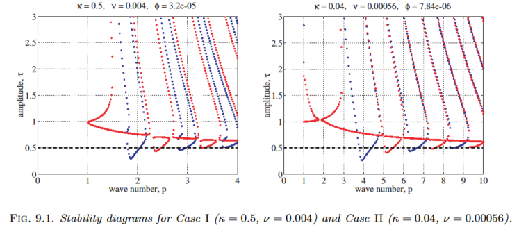
Figure A: Original stability contours for cases I and II, reproduced from [1].

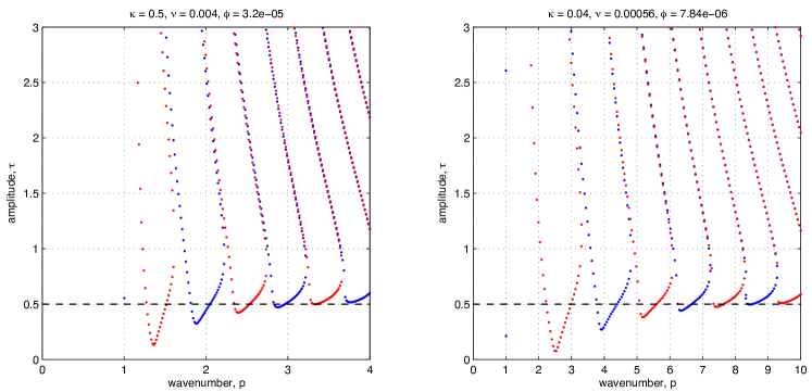
Figure B: Corrected stability contours for cases I and II (compare to Figure A).

Each point depicted in these plots represents one solution to the eigenvalue problem formulated in Eq. (8.1) of [1], and the stability boundaries are traced out by varying the angular wavenumber ($p$) of the circular fiber. The blue points denote harmonic modes and the red points denote subharmonic modes. The only “physical” instabilities are those corresponding to integer values of wavenumber $p$ that lie inside the stability “tongues” and satisfy $0\leqslant\tau\leqslant\frac{1}{2}$. With this in mind, the lowest wavenumber unstable mode in case I corresponds to $p=2$, while that in case II has $p=4$.

Other than the discrepancies noted above, the original stability plots from [1] are still qualitatively correct and the parametric resonances identified in the original paper are also true instabilities (as verified in numerical simulations). Nevertheless, we have performed new calculations with the corrected Matlab code that demonstrate the existence of resonant subharmonic modes that were not identified in the original paper. New resonant modes occur only when the missing subharmonic region overlaps with an integer value of $p$, which is not the case in the two examples plotted in Figures A and B. The original stability plots from Figures 8.2 and 8.3 are reproduced in Figure C while our corrected plots are given in Figure D. In all cases, the spurious points are eliminated and a new subharmonic mode appears.

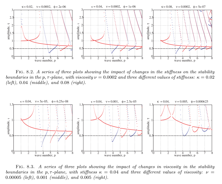
Figure C: Original stability plots, reproduced from [1].

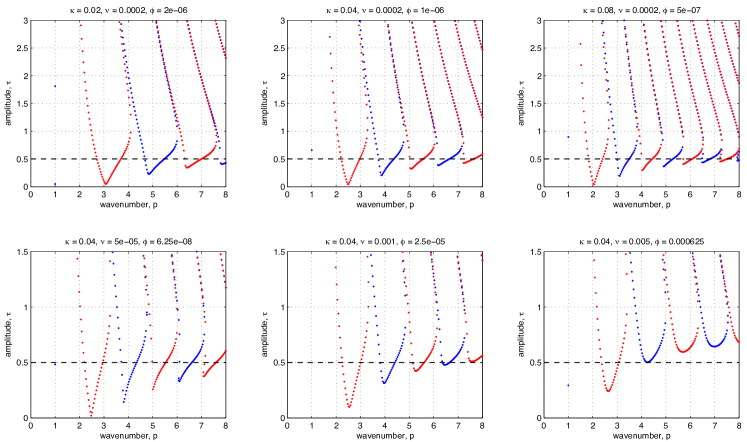
Figure D: Corrected stability plots (compare to Figure C).

To illustrate the presence of the missing unstable modes, we choose the following two sets of parameters listed below

Case III	Case IV
$\kappa=0.02$	$\kappa=0.08$
$\nu=0.0002$	$\nu=0.0002$
$\phi=2\times 10^{-6}$	$\phi=5\times 10^{-7}$

which correspond (respectively) to the left- and right-most plots in Figures 8.2-8.3. Numerical simulations of the full immersed boundary equations have been performed for Case III (with $p=3$) and Case IV (with $p=2$) to verify that these parametric resonances are actual instabilities. Following the approach used in [1], we initialize the fiber using the perturbed circular shape $r=R(1+0.05\cos(p\theta))$, where $p$ is chosen equal to the resonant wavenumber. Figure E shows the amplitude of various $p$-modes in the two simulations, from which it is clear that the resonant mode is excited and its amplitude grows in time, as would be expected for the resonant case. The amplitude of the other modes remains small.

(a)

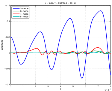
(b)

Figure E: Amplitudes of the various $p$-modes from numerical simulations of Cases III (left, $p=3$ unstable) and IV (right, $p=2$ unstable).

Other than the presence of these missing lowest-wavenumber subharmonic modes, the effect on the stability contours is relatively small for the parameter values we considered. Figure F draws a direct comparison between the stability regions for cases I and II obtained with the original equations and with the corrected equations. Clearly, the correction results in only a small deformation in the contours and thus has only minimal impact on the solution. All other cases considered in [1] yield similar results.

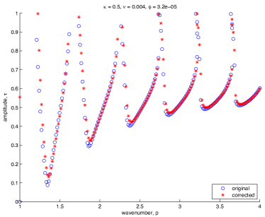
(a)

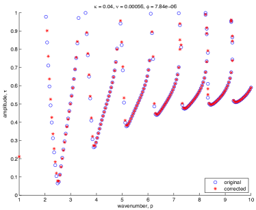
(b)

Figure F: Comparison of the eigenvalue plots for the original (blue) and corrected (red) equations in Cases I (left) and II (right).

References

- [1] R. Cortez, C. S. Peskin, J. M. Stockie, and D. Varela. Parametric resonance in immersed elastic boundaries. SIAM Journal on Applied Mathematics, 65(2):494–520, 2004.
- [2] S. Hassani. Dirac delta function. In Mathematical Methods for Students of Physics and Related Fields, chapter 5, pages 139–170. Springer, New York, 2009. http://dx.doi.org/10.1007/978-0-387-09504-2_5.