Lensing degeneracies and mass substructure

Abstract

The inversion of gravitational lens systems is hindered by the fact that multiple mass distributions are often equally compatible with the observed properties of the images. Besides using clear examples to illustrate the effect of the so-called monopole and mass sheet degeneracies, this article introduces the most general form of said mass sheet degeneracy. While the well known version of this degeneracy rescales a single source plane, this generalization allows any number of sources to be rescaled. Furthermore, it shows how it is possible to rescale each of those sources with a different scale factor. Apart from illustrating that the mass sheet degeneracy is not broken by the presence of multiple sources at different redshifts, it will become apparent that the newly constructed mass distribution necessarily alters the existing mass density precisely at the locations of the images in the lens system, and that this change in mass density is linked to the factors with which the sources were rescaled. Combined with the fact that the monopole degeneracy introduces a large amount of uncertainty about the density in between the images, this means that both degeneracies are in fact closely related to substructure in the mass distribution. An example simulated lensing situation based on an elliptical version of a Navarro-Frenk-White profile explicitly shows that such degeneracies are not easily broken by observational constraints, even when multiple sources are present. Instead, the fact that each lens inversion method makes certain assumptions, implicit or explicit, about the smoothness of the mass distribution means that in practice the degeneracies are broken in an artificial manner rather than by observed properties of the lens system.

1 Introduction

Not only can strong gravitational lensing yield impressive images, from multiply imaged quasars over deformed galaxies to partial or full Einstein rings, it is also an invaluable tool to estimate the mass of the deflector. Moreover, since the precise positions and deformations of the images of a source depend on the exact distribution of the mass, gravitational lensing even holds the promise of constraining the shape of said mass distribution.

In principle, this strong lens inversion sounds fairly straightforward: use a particular model and optimize its parameters so that it reproduces the observations as well as possible. In practice however, one is hindered by gravitational lensing degeneracies which allow a wide range of mass distributions to produce the exact same image configuration. On the level of parametric lens inversion results, this can manifest itself as parameter degeneracies (e.g. Wambsganss & Paczynski (1994)), but at their core the degeneracies are or course present at the level of the mass distribution. There, the mass sheet degeneracy (e.g. Falco et al. (1985) or Saha & Williams (2006)) will rescale the projected mass distribution while adding a constant density mass sheet (or disc), only affecting the time delays between the images. Recently it was shown that a similar procedure is still possible when multiple sources at different redshifts are observed (Liesenborgs et al., 2008a). While this degeneracy therefore can still be broken when time delay measurements are present, the situation is far worse with respect to the so-called monopole degeneracy (Liesenborgs et al., 2008b). This type of degeneracy can be used to redistribute the mass in between the images, without changing any of the observable properties of the images.

By presenting a further generalization of this mass sheet degeneracy, this article will illustrate an important relation between different degenerate versions of a lensing mass distribution. This will illustrate how degeneracies are closely related to the substructure in the mass density, which, in turn, offers insights into what one may constrain about the lensing mass.

After briefly introducing the lensing formalism and used notations in section 2, the basics of the monopole and mass sheet degeneracies are reviewed in section 3. This will serve as the starting point for some extensions in section 4 after which an experiment in section 5 will illustrate precisely how difficult it can be to estimate the parameters of a specific type of mass distribution, an elliptical generalization of a Navarro-Frenk-White profile (Navarro et al., 1996). Finally, in section 6 we shall discuss what the implications of these degeneracies are and what different types of information can help constrain.

2 Lensing formalism

In this section, the same notation as Schneider et al. (1992) is used, which the interested reader can consult for a thorough review. The lens equation (1) in essence states that due to the gravitational deflection $\hat{\alpha}$ of a light ray, when looking in a direction $\theta$ one sees what would be observed in direction $\beta$ if the lens effect could be turned off:

$$\mbox{\boldmath$\beta$}(\mbox{\boldmath$\theta$})=\mbox{\boldmath$\theta$}-\frac{D_{\rm ds}}{D_{\rm s}}\mbox{\boldmath$\hat{\alpha}$}(\mbox{\boldmath$\theta$})\mathrm{.}$$ (1)

The deflection angle $\hat{\alpha}$ depends on the two-dimensional projected mass distribution $\Sigma$ in the following fashion:

$$\mbox{\boldmath$\hat{\alpha}$}=\frac{4GD_{\rm d}}{c^{2}}\int\frac{\Sigma(\mbox{\boldmath$\theta^{\prime}$})(\mbox{\boldmath$\theta$}-\mbox{\boldmath$\theta^{\prime}$})}{\left|\mbox{\boldmath$\theta$}-\mbox{\boldmath$\theta^{\prime}$}\right|^{2}}d\mbox{\boldmath$\theta^{\prime}$}\mathrm{.}$$ (2)

In these equations, the geometry of the lensing scenario is given by the angular diameter distances $D_{\rm d}$, $D_{\rm s}$ and $D_{\rm ds}$, describing the distance to the lens, to the source and the distance between lens and source respectively. It will often be convenient to use the so-called critical density:

$$\Sigma_{\rm cr}=\frac{c^{2}}{4\pi G}\frac{D_{\textrm{s}}}{D_{\textrm{ds}}D_{\textrm{d}}}\mathrm{,}$$ (3)

which depends on the redshift of a source through the angular diameter distances involved.

In the special case of a circularly symmetric mass distribution, for convenience assumed to be centered on the origin of the coordinate system, the expression of the deflection angle reduces to:

$$\mbox{\boldmath$\hat{\alpha}$}(\mbox{\boldmath$\theta$})=\frac{4GM(\theta)}{c^{2}D_{\rm d}\theta^{2}}\mbox{\boldmath$\theta$}\mathrm{,}$$ (4)

in which $M(\theta)$ represents the mass enclosed within radius $\theta$:

$$M(\theta)=2\pi D_{\rm d}^{2}\int_{0}^{\theta}\Sigma(\theta^{\prime})\theta^{\prime}d\theta^{\prime}\mathrm{.}$$ (5)

The deflection angle can be shown to be proportional to the gradient of the so-called lens potential

$$\mbox{\boldmath$\nabla$}\psi(\mbox{\boldmath$\theta$})=\frac{D_{\rm ds}}{D_{\rm s}}\mbox{\boldmath$\hat{\alpha}$}(\mbox{\boldmath$\theta$})\mathrm{,}$$ (6)

which is related to the time light takes to travel from the source at position $\beta$ to an image at position $\theta$:

$$t\left(\mbox{\boldmath$\theta$}\right)=\frac{1+z_{\rm d}}{c}\frac{D_{\rm d}D_{\rm s}}{D_{\rm ds}}\left(\frac{1}{2}\left(\mbox{\boldmath$\theta$}-\mbox{\boldmath$\beta$}\right)^{2}-\psi(\mbox{\boldmath$\theta$})\right)+\mathrm{const}\mathrm{.}$$ (7)

In this last equation, $z_{\rm d}$ is the redshift of the gravitational lens. Since, in practice one is only interested in the difference in time delay between images of the same source, the constant in this expression is of no importance. The curvature of the lens potential can be shown to represent the mass density at the corresponding point:

$$\frac{1}{2}\nabla^{2}\psi\left(\mbox{\boldmath$\theta$}\right)=\frac{\Sigma\left(\mbox{\boldmath$\theta$}\right)}{\Sigma_{\rm cr}}\mathrm{.}$$ (8)

Finally, the magnification $\mu$ that an image at position $\theta$ experiences, can be calculated from the lens equation as follows:

$$\mu^{-1}\left(\mbox{\boldmath$\theta$}\right)=\left|\frac{\partial\beta_{i}}{\partial\theta_{j}}\right|\mathrm{,}$$ (9)

i.e. it is the jacobian determinant of this equation.

3 Degeneracy basics

3.1 Monopole degeneracy

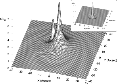
Figure 1: Left panel: this non-singular isothermal ellipse based gravitational lens transforms a single source into the five images that can be seen in the left panel of Fig. 2. Right panel: when the mass distribution shown in the inset is added in the region enclosed by a circle in Fig. 2 (left panel), this mass distribution is created. Note that although the added mass distribution itself contains a region of negative density, the total density of the lens is positive everywhere.

Figure 2: Left panel: the gravitational lens shown in the left panel of Fig. 1 creates five images of the source enclosed by a small square. A circle encloses a region which does not contain any of the images, and can therefore be used to illustrate the monopole degeneracy (see text). Right panel: when the circularly symmetric mass distribution from the inset of Fig. 1 is added in the circular region, the resulting mass distribution (right panel of Fig. 1) still maps the source onto the exact same images. Note that the change in the critical lines and caustics illustrates the fact that inside the circular region, the lens equation indeed has changed.

The so-called monopole degeneracy, first mentioned in Saha (2000) and studied in more detail in Liesenborgs et al. (2008b), is both the least complex and most elusive degeneracy one can think of. Consider the mass distribution shown in the inset in Fig. 1. Being a circularly symmetric mass distribution, its lens effect is governed by equation (4). Since this particular mass distribution was constructed to have zero enclosed mass outside a particular radius, the same equation shows that it will not cause a deflection angle outside said radius. This kind of mass density will be referred to as a monopole, since it can be described by only the monopole term in a multipole expansion.

An example will illustrate the importance of such a monopole. The elliptical mass distribution shown in the left panel of Fig. 1 transforms a single source into five distinct images, as can be seen in the left panel of Fig. 2. Indicated in the same figure, is a circular region in which none of the images are located, and which has the precise same diameter as the aforementioned monopole. When adding the monopole in this location, this implies that the lens equation will not be affected outside the circular region; only within will the deflection of light be affected. That this is indeed the case, can clearly be seen in the right panel of Fig. 2. There, the lens effect is calculated for the same source, but for the combined mass distribution shown in the right panel of Fig. 1. As was expected, the exact same five images are generated by this clearly different mass density. The fact that the lens equation was modified inside the circular region can be seen in the change in critical lines in this region. Since the deflection is different inside the circular area, in principle it is even possible that extra images are generated there. However, this particular example shows that this does not necessarily need to be the case, even for a rather large modification of the mass distribution.

This example already shows that by ‘borrowing’ some mass from a relatively large region, it is easy to introduce (or remove) a mass peak in a mass density, without changing the images that are generated. As was explicitly shown in (Liesenborgs et al., 2008b) however, it is also possible to use such monopoles as basis functions which allows a complex redistribution of the mass by adjusting their weights. As long as no basis function overlaps with an image, none of the images will be affected by this operation. Some care needs to be taken not to introduce additional, unobserved images though.

From the discussion above, it is already trivially clear that this type of degeneracy does not modify the image positions generated by a particular source. The fact that the deflection angle is zero outside a certain radius, by equation (9) implies that the magnification at the location of the images will not be affected either. Equation (6) on the other hand shows that the lens potential outside said radius may change by a constant value. However, when measuring time delays between images, such a constant offset in the potential will have no effect, as can be seen in equation (7).

3.2 The mass sheet degeneracy

The mass-sheet degeneracy is undoubtedly one of the most famous degeneracies in gravitational lensing. Contrary to what the name may suggest, to obtain a degenerate solution it is not sufficient to simply add a sheet of mass to an existing mass distribution. Instead, one has to rescale the original mass distribution as well, prompting the use of the alternative name of steepness degeneracy (Saha & Williams, 2006).

Figure 3: The mass sheet degeneracy in its simplest form causes a rescaled version of the source plane to correspond to the same images. The fact that the entire source plane has been rescaled is most obvious when comparing the caustics to those of the left panel of Fig. 2. In this particular example, a value of $\lambda=0.7$ was used in the construction of a degenerate solution according to equation (11).

As a concrete example, let us call the mass distribution of the left panel of Fig. 1 $\Sigma_{0}$, producing a deflection field $\mbox{\boldmath$\hat{\alpha}$}_{0}$. Using equation (4), one can show that for a sheet of mass of precisely the critical density $\Sigma_{\rm cr}$, the deflection angle simply becomes:

$$\mbox{\boldmath$\hat{\alpha}$}_{\rm s}\left(\mbox{\boldmath$\theta$}\right)=\frac{D_{\rm s}}{D_{\rm ds}}\mbox{\boldmath$\theta$}\mathrm{.}$$ (10)

If one then constructs a new mass density $\Sigma_{1}$ as follows:

$$\Sigma_{1}\left(\mbox{\boldmath$\theta$}\right)=\lambda\Sigma_{0}\left(\mbox{\boldmath$\theta$}\right)+(1-\lambda)\Sigma_{\rm cr}\mathrm{,}$$ (11)

it is a straightforward exercise to show that for the combined deflection $\lambda\mbox{\boldmath$\hat{\alpha}$}_{0}+(1-\lambda)\mbox{\boldmath$\hat{\alpha}$}_{\rm s}$ the new lens equation is:

$$\mbox{\boldmath$\beta$}_{1}\left(\mbox{\boldmath$\theta$}\right)=\lambda\mbox{\boldmath$\beta$}_{0}\left(\mbox{\boldmath$\theta$}\right)\mathrm{,}$$ (12)

i.e. merely a rescaling of the original one. This means that a rescaled version of the source plane corresponds to the same images, as is illustrated in Fig. 3.

If the source involved is variable, it may be possible to measure time delays between the images:

$$\Delta t_{ij}=t(\mbox{\boldmath$\theta$}_{i})-t(\mbox{\boldmath$\theta$}_{j})\mathrm{,}$$ (13)

where $\mbox{\boldmath$\theta$}_{i}$ and $\mbox{\boldmath$\theta$}_{j}$ are the positions of two of the images. For a sheet of mass consisting of precisely the critical density, the projected potential is

$$\psi_{s}(\theta)=\frac{1}{2}\theta^{2}\mathrm{,}$$ (14)

so that the mass sheet degeneracy transforms an initial lens potential $\psi_{0}$ into

$$\psi_{1}(\mbox{\boldmath$\theta$})=\lambda\psi_{0}(\mbox{\boldmath$\theta$})+\frac{1-\lambda}{2}\theta^{2}\mathrm{.}$$ (15)

Noting that the mass sheet degeneracy changes a source position $\mbox{\boldmath$\beta$}_{0}$ to $\mbox{\boldmath$\beta$}_{1}=\lambda\mbox{\boldmath$\beta$}_{0}$, a brief calculation shows that the relationship between the original time delay $\Delta t_{ij,0}$ and the time delay of the degenerate version $\Delta t_{ij,1}$ becomes:

$$\Delta t_{ij,1}=\lambda\Delta t_{ij,0}\mathrm{.}$$ (16)

This means that time delay measurements break this mass sheet degeneracy, since a particular version of the degeneracy corresponds to a particular time delay.

Figure 4: In this example, two sources at a different redshift each produce two images due to the presence of a gravitational lens. Because of the different redshifts, each source would require a different critical density in the construction of a solution that differs by the mass sheet degeneracy. The enclosed mass profiles corresponding to these two densities are shown as curves $M_{\rm A}$ and $M_{\rm B}$. The locations of the images of each source are indicated on these profiles. The dashed line, an interpolation between the two curves, shows a total mass profile that effectively behaves as the two sheets, from the perspective of the images (see text).

The mass sheet degeneracy also has a particularly simple effect on the magnification factor $\mu$. Since each dimension is scaled by a factor $\lambda$, the surface area of a small source is scaled by a factor $\lambda^{2}$. Keeping the sizes of the images constant, this means that the new magnifications of the source are given by $\mu_{1}=\lambda^{-2}\mu_{0}$. This result can also be obtained by combining the general expression for the magnification (9) and the relation between the degenerate versions of the lens equation (12).

4 Generalized mass sheet degeneracy

A first generalization of the mass sheet degeneracy was described in Liesenborgs et al. (2008a). A brief review shall be presented here, before discussing an even more general version of this degeneracy. It has often been claimed that having two distinct sources at different redshifts breaks the mass sheet degeneracy. From the construction above, the reason for this is clear. A sheet with precisely the critical density was used, but since the critical density is redshift dependent, each source would now require the use of a sheet with a different density.

This situation is illustrated in Fig. 4. Source $A$ would require a sheet of mass which gives rise to the enclosed mass profile $M_{\rm A}(\theta)$. Similarly, source $B$ would need a sheet with mass profile $M_{\rm B}(\theta)$. The radii at which images of each source are present are indicated on the corresponding mass profile. While it is true that a single mass sheet can no longer be used for a construction like the one in equation (11), it indeed is possible to construct a mass density that for each source has the same effect as its corresponding mass sheet.

The key point is that for a circularly symmetric mass distribution, equation (4) shows that the deflection angle is caused by the total enclosed mass within a specific radius, without any dependence on the structure of the mass profile within said radius. This implies that if one were to construct the mass profile indicated by the dashed line in Fig. 4, the deflection angle at the location of the images of source $A$ will be the same as when caused by a mass sheet of precisely its critical density. Similarly, the images of source $B$ will effectively ‘see’ a mass sheet with their critical density. The mass density corresponding to this new profile can then be used to construct a degenerate solution in the same way as in equation (11). Calling $R_{\rm A}$ and $R_{\rm B}$ the radii at which images of sources $A$ and $B$ are located, by construction this implies that:

$$\Sigma_{1}\left(R_{\rm A}\right) = \lambda\Sigma_{0}\left(R_{\rm A}\right)+(1-\lambda)\Sigma_{\rm cr}\left(z_{\rm A}\right)$$

$$\Sigma_{1}\left(R_{\rm B}\right) = \lambda\Sigma_{0}\left(R_{\rm B}\right)+(1-\lambda)\Sigma_{\rm cr}\left(z_{\rm B}\right)\mathrm{.}$$ (17)

Figure 5: Left column: this gravitational lensing situation is used as a starting point to illustrate the general mass sheet degeneracy in which different sources are scaled with different values. The top figure depicts the elliptical mass distribution of the gravitational lens; the two other figures show how this lens creates three images of two different sources. In this example, only the source in the middle panel (source $A$) will be rescaled, the source in the bottom figure (source $B$) will not. Center column: after modifying the mass distribution in the left column using the method of the monopole basis functions (see text), a rescaled version of source $A$ is needed to create the same images as before. Source $B$ on the other hand does not need to be altered to recreate the same image configuration. To illustrate that the source plane of source $A$ has been rescaled toward the origin can be seen by comparing the new source position to the original one. Right column: similar to the center column, but in this case a similar interpolation method for the deflection field was used as in the LensPerfect lens inversion procedure (Coe et al., 2008).

The effect is the same as for the original mass sheet degeneracy: the images will now correspond to sources which are rescaled by the same factor $\lambda$. The magnifications are therefore again modified by $\lambda^{-2}$. The effect on the time delay is not as straightforward however. For a circularly symmetric lens, combining equations (6) and (4) shows that

$$\psi(\theta)\propto\int_{0}^{\theta}\frac{M(\theta^{\prime})}{\theta^{\prime}}d\theta^{\prime}\mathrm{,}$$ (18)

i.e. the lens potential, and therefore the time delays, will depend on the precise manner in which the interpolation between the two curves in Fig. 4 is done.

Using the generalization of the mass sheet degeneracy that was just shown, the sources are still rescaled with the same factor. But it is also possible to construct a degenerate solution which allows one to scale each source with a different factor. To illustrate this, consider the situation shown in the left panel Fig. 5: an elliptical mass distribution causes two sources to produce three images each. In what follows, only source $A$ will be rescaled with a certain factor. In a subsequent step the other source can be rescaled in a similar way, using a different factor.

Focusing on only one source and temporarily forgetting about the other, the source can be rescaled using the classic mass sheet degeneracy from equation (11). This means that to the initial $\Sigma_{0}$, a mass distribution $\Sigma_{\rm add}$ was added to obtain $\Sigma_{1}$:

$$\Sigma_{\rm add}(\mbox{\boldmath$\theta$})=(1-\lambda)\left[\Sigma_{\rm cr}(z_{\rm A})-\Sigma_{0}(\mbox{\boldmath$\theta$})\right]\mathrm{.}$$ (19)

Taking the second source back into account, it is clear that adding $\Sigma_{\rm add}$ to the original mass distribution will cause the images of source $A$ to correspond to a scaled version of that source, but the effect on the second source is less desirable.

However, suppose it is possible to modify $\Sigma_{\rm add}$ so that the deflection it causes for source $A$ is unaltered, and no deflection is caused at the location of the images of source $B$. In that case, after adding $\Sigma_{\rm add}$, the images of source $A$ would correspond to a scaled version of that source, and the images of source $B$ would still be projected onto the same source area. Calling $I_{\rm A}$ and $I_{\rm B}$ the points of which respectively the images of sources $A$ and $B$ consist, $\mbox{\boldmath$\hat{\alpha}$}_{\rm add}(I_{\rm B})=0$ by equations (6) and (8) implies that $\Sigma_{\rm add}(I_{\rm B})=0$. If one then constructs $\Sigma_{1}=\Sigma_{0}+\Sigma_{\rm add}$, in general one finds that

$$\Sigma_{1}(I_{\rm A}) = \lambda\Sigma_{0}(I_{\rm A})+(1-\lambda)\Sigma_{\rm cr}(z_{\rm A})$$

$$\Sigma_{1}(I_{\rm B}) = \Sigma_{0}(I_{\rm B})$$ (20)

Starting from $\Sigma_{1}$, in a next step one can then exchange the roles of the two sources and rescale source $B$ with a different factor.

There still remains the question of how to modify $\Sigma_{\rm add}$ so that it does not produce a deflection at the location of the images of source $B$. This can be done by using a large number of the monopole basis functions we met earlier. If none of these overlap with the images of source $A$, the deflection there will be unaltered. To make sure that the deflection angle at the location of the images of source $B$ vanishes, appropriate weights of these basis functions must be sought. An example of this approach can be seen in the center panel of Fig. 5. In this example, the weights were determined by a genetic algorithm, an optimization strategy inspired by natural selection. A similar procedure is used as in Liesenborgs et al. (2008b): a trial solution consists of a set of weights for the monopole basis functions. Starting from randomly initialized trial solutions, the algorithm then ‘breeds’ increasingly better trial solutions by combining existing solutions and introducing mutations. A key step in this procedure is the application of selection pressure: better solutions should produce more offspring. In this case, a trial solution is deemed better than another simply when its deflection field differs less from the desired one at the locations of the images of source $B$. Since, when generating a degenerate solution in this fashion, one still uses a rescaled version of the original mass distribution, this procedure still produces a mass map which appears rescaled, as can be seen in the center panel of Fig. 5.

Another approach which does not cause such an apparent rescaling, can be used as well. From the discussion above, it is clear that the final version of the mass distribution $\Sigma_{\rm add}$ should produce a specific value of the deflection angle $\mbox{\boldmath$\hat{\alpha}$}_{\rm add}$ at the location of the images of source $A$. On the other hand, at the location of the images of source $B$, no deflection should be produced. We therefore know the deflection angle at specific locations, and at other locations the deflection angle can take a large number of values, the only real constraint being that no additional images should be produced. Interpolating a deflection field in such a way that $\mbox{\boldmath$\nabla$}\times\mbox{\boldmath$\hat{\alpha}$}_{\rm add}=0$, or equivalently that the deflection originates from a scalar lensing potential, is precisely what is done in the LensPerfect lens inversion procedure (Coe et al., 2008). Using a similar interpolation procedure to determine $\mbox{\boldmath$\hat{\alpha}$}_{\rm add}$ and therefore $\Sigma_{\rm add}$, yields the result shown in the right panel of Fig. 5. While more difficult to ensure that the overall mass distribution is positive, in this example it produces an interesting result. Comparing the resulting mass distribution with the original one in the left panel, one sees that the differences are rather subtle. And since no rescaling of the mass density itself seems to be involved, one would not suspect a mass sheet-like degeneracy to be at work here.

Note that in principle, a similar construction is possible when only using point sources. When the deflection angles are only conserved at very specific point locations and not over a more extended area, the gradients of the deflection field will change and therefore also the surface density and the magnification factors. In particular, the relation in equation (20) will no longer hold. However, since this no longer corresponds to a rescaling of the sources, it can hardly be considered as caused by the mass sheet degeneracy.

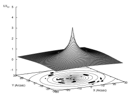
Figure 6: Left panel: the input mass distribution for a simulated lensing scenario consists of an elliptical generalization of a NFW profile. Eight distinct sources generate 26 images which are shown on top of the contour map. Center panel: for a source at $z=3$, the mass distribution from the left panel generates these critical lines and caustics. Right panel: the same 26 input images as in the left panel are shown here. The three images of a single source which will be used for additional time delay constraints later, are surrounded by squares.

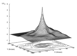
Figure 7: Left panel: when only positional information about the image systems is used and only Plummer basis functions are used, corresponding to the algorithm as described in Liesenborgs et al. (2006), the average of 20 individual solutions yields this mass distribution. Although the overall shape is similar to the mass distribution in Fig. 6, this mass map is clearly much more steep. Center panel: the critical lines and caustics for this average solution. Comparing this to the center panel of Fig. 6, one immediately notices that the scale of the caustics is much larger, indicating the presence of a mass sheet-like degeneracy. Right panel: the densities of the individual solutions are compared to the true input mass densities, precisely at the locations of the image centers. Being much more steep and apparently lacking a constant offset again reveals the presence of a mass sheet-like degeneracy.

5 Experiment

5.1 Positional information

To further illustrate the significant practical problems posed by these degeneracies, we shall use a simulated lensing scenario. The left panel of Fig. 6 shows the true mass map used in the simulation, an elliptical generalization of a NFW mass distribution (Navarro et al., 1996; Wright & Brainerd, 2000), with concentration parameter $c_{\rm vir}=5$ and scale parameter $r_{\rm s}=50$ arcseconds. The lens was placed at a redshift of $0.7$ in a cosmology with $H_{0}=70$ km s^-1 Mpc^-1, $\Omega_{\rm m}=0.3$ and $\Omega_{\Lambda}=0.7$. The surface density is expressed in terms of the critical density for a source at $z=3$. Eight sources were placed at different redshifts. These generate 26 images which can be seen in the contour map, and also in the right panel of the same figure. The redshifts of the sources lie between $z=2.7$ and $z=3.4$. The center panel of Fig. 6 shows the critical lines and caustics for a source at $z=3$. We shall be interested in comparing the scale of the caustics here to that of reconstructions, as rescaling the source plane is the hallmark of the mass sheet degeneracy.

First, a reconstruction is done using the algorithm presented in Liesenborgs et al. (2006). In this method, Plummer (Plummer, 1911) basis functions are arranged according to an adaptive grid, and the weights of these basis functions are determined using a genetic algorithm. The left panel of Fig. 7 shows the resulting mass distribution, an average of 20 individual reconstructions. Overall, it has a similar appearance as the input mass map shown in Fig. 6, and its critical lines (center panel) do bear resemblance to those of the true lens. The resulting mass distribution, however, is considerably steeper than the one used in the simulation, which can also clearly be seen in the right panel of Fig. 7. In this image we show the densities measured at the center of each image. For the sake of visualization, instead of using the two dimensional coordinate of each image center point, the distance to the NFW center is used on the $x$-axis. Comparing the two profiles on that figure, one is immediately reminded of the mass sheet degeneracy, i.e. the profiles seem to differ mostly by a rescaling and the addition of a specific offset. Similarly, when looking at the caustics in the center panel of Fig. 7, they seem to be an expanded version of the ones of the input lens, again a feature that hints at the presence of the mass sheet degeneracy.

Due to the inherent uncertainty in between the images caused by the monopole degeneracy, the most sensible thing to do in trying to retrieve the NFW parameters, is to perform a fit based on the densities precisely at the locations of the images. When looking at the steepness of the reconstructed mass map, it will come as no surprise that extracting the concentration and scale parameters from the reconstructed densities will not yield accurate results. In this particular case, the estimates are $c_{\rm vir}=14.1^{+0.6}_{-0.5}$ and $r_{\rm s}=11.7^{+0.6}_{-0.7}$ arcseconds respectively (68% confidence level).

Figure 8: Left panel: to generate this average solution, the same algorithm was used as in Fig. 7, but this time a constant density sheet was allowed as a basis function as well (see Liesenborgs et al. (2009)). This solution resembles the input mass distribution more closely. Center panel: when the critical lines and caustics for this solution are calculated, the source plane no longer exhibits an obvious rescaling compared to the input situation. Right panel: comparing the densities at the image centers to those of the input mass map confirms that this reconstruction is much more similar to the true situation than the mass distribution from Fig. 7.

Using Plummer basis functions it is of course rather difficult to mimic the effect of a sheet of mass. Given the fact that within the images a considerable mass sheet-like component seems to be present in the input lens, the fact that the reconstruction is rather different is not that surprising. In a second reconstruction not only Plummer basis functions were used, but a single mass sheet basis function was present as well, as is also explained in Liesenborgs et al. (2009). The resulting mass distribution, again an average of 20 individual solutions, can be seen in the left panel of Fig. 8. This mass distribution is clearly a lot more similar to the input mass map, also obvious from the right panel of the same figure. As can be expected from the similarity between the true and reconstructed lenses, the caustics shown in the center panel no longer show a clear difference in scale. When performing a fit in a similar fashion as the previous reconstruction, one finds NFW parameters of $c_{\rm vir}=5.9^{+0.6}_{-0.5}$ and $r_{\rm s}=38.3^{+4.9}_{-4.4}$ arcseconds, corresponding better to the true values.

Unfortunately, in this example there is no real reason to prefer one reconstruction over the other, meaning that apart from the overall shape of the true mass distribution, little would be revealed by performing these inversions. Furthermore, in both cases fitting the NFW shape yields an overestimate of the concentration parameter and an underestimate of the scale radius, although the effect is far more serious in the first inversion.

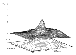
Figure 9: Left panel: this is the average solution when only Plummer basis functions are used, similar to Fig. 7, but as an additional constraint the time delays between the images indicated in the right panel of Fig. 6 were included. Comparing this result to the one in Fig. 7 reveals that the addition of this information has a profound effect on the steepness of the solution. Center panel: thanks to the presence of the time delay information the caustics of this average solution no longer display the obvious rescaling that could be observed earlier. Right panel: as was already suggested by the left panel, comparing the densities at the image locations shows that the time delay information for even a single image system seems to pull all reconstructed densities towards the true densities.

Figure 10: Left panel: when both time delay information about the system marked in the right panel of Fig. 6 and a mass sheet basis function are allowed, this average result is obtained. Apart from the sharp central peak, the mass distribution is very similar to the input mass map. Center panel: calculating the critical lines and caustics of this solution reveals that the source plane is very similar in scale to the one of the input lens. Right panel: in this case the densities at the image locations are extremely similar to the input densities. Only the density at the point closest to the center of the input NFW distribution appears to be underestimated systematically.

5.2 Including time delay information

Earlier in this article it was mentioned that time delay information can help not only in breaking the most basic mass sheet degeneracy; also for the generalized versions time delays depend on the precise construction method of the degenerate mass map. In Liesenborgs et al. (2009) a method was described with which time delay information can be added as a constraint, now using a so-called multi-objective genetic algorithm. To explore the value of such time delays, time delay information of a single system of images was added to the inversion procedure. The three images used for this added constraint are indicated in the right panel of Fig. 6 and correspond to a lensed source at redshift 2.75.

First, the inversion was run using Plummer basis functions alone, i.e. no mass sheet basis function was used. The resulting mass distribution can be seen in the left panel of Fig. 9. Concerning the input to the inversion procedure, the only difference with the results obtained in Fig. 7 is the addition of time delay information. The effect of this information is impressive however: especially when comparing the right panels of these two figures it is clear that the time delay constraint seems to pull the densities at all image locations towards the true densities. The caustics in the center panel confirm the mass sheet-breaking effect: the overall scale of the source plane seems to match the true one more closely. Note that this is solely the effect of time delays for a single image system. When determining the NFW parameters as before, one now finds $c_{\rm vir}=7.4^{+0.6}_{-0.5}$ and $r_{\rm s}=28.8^{+2.8}_{-2.9}$ arcseconds. This result still does not reflect the true parameters, but is far less deviant than the estimates based on Fig. 7.

As a final inversion, both the time delay information and the mass sheet basis function was used, i.e. the inversion is similar to the one reflected by Fig. 8, but now including time delay information about one set of images. The resulting mass map is depicted in the left panel of Fig. 10; the densities at the image locations can be seen in the right panel of the same figure. The effect of the added time delay information is not as impressive as in the previous example, but still it leads to an improvement of the estimated densities at most image points. Only the density at the point closest to the NFW center seems to be underestimated systematically. This single outlier does not seem to have a profound adverse effect on the estimation of NFW parameters however, which now are $c_{\rm vir}=4.8^{+0.4}_{-0.3}$ and $r_{\rm s}=52.1^{+5.2}_{-4.1}$ arcseconds, very close to the true values.

6 Discussion and conclusion

The examples shown in this article make it clear that these lensing degeneracies are closely related to substructure in the mass density. The monopole degeneracy is the worst, as it has no effect on any property of the images: the same sources predict the same images, with identical magnifications and identical time delays. In essence it means that we do not have a firm handle on the mass distribution in between the images, the only real constraint being the absence of unobserved images. This illustrates both the importance of gravitational lens systems with a multitude of images and when necessary, of the use of the null space, i.e. the locations where no images are observed.

In its most general version, the mass sheet degeneracy does not require an actual sheet of mass, nor does it necessarily modify the slope of the mass distribution, as the alternative name of steepness degeneracy might suggest. Comparing equations (11), (17) and (20), it becomes clear that when scaling source $A$ with factor $\lambda_{\rm A}$ and source $B$ with factor $\lambda_{\rm B}$, the effect on the mass density is the following:

$$\Sigma_{1}\left(I_{\rm A}\right) = \lambda_{\rm A}\Sigma_{0}\left(I_{\rm A}\right)+(1-\lambda_{\rm A})\Sigma_{\rm cr}\left(z_{\rm A}\right)$$

$$\Sigma_{1}\left(I_{\rm B}\right) = \lambda_{\rm B}\Sigma_{0}\left(I_{\rm B}\right)+(1-\lambda_{\rm B})\Sigma_{\rm cr}\left(z_{\rm B}\right)\mathrm{,}$$ (21)

where $I_{\rm A}$ and $I_{\rm B}$ are again the locations of the images of source $A$ and $B$ respectively. Of course, this can be generalized to any number of sources and images. Apart from rescaling each source in the system, equation (21) illustrates that this degeneracy changes the density precisely at the locations of the images, i.e. it necessarily introduces substructure. The effect on the time delays is in general not straightforward implying that time delay information may be very valuable in helping to break this degeneracy. The simple effect on the magnification is not easy to use since one most often does not have information about the size of the source. Efforts to use the magnification information to avoid the mass sheet degeneracy have been undertaken however, e.g. in Taylor et al. (1998).

The fact that both monopole and mass sheet degeneracies are – at least in principle – possible with any amount of sources and images, combined with the fact that they are both linked to substructure in the mass distribution, means that in reality it is the prior information on the degree of smoothness of the mass distribution that effectively breaks these degeneracies. The degree of smoothness can depend implicitly on the method used, e.g. in parametric methods like the LensTool method (Jullo et al., 2007), the method of Zitrin et al. (2010) which is largely based on the distribution of the light, or the method of the authors in which overlapping smooth basis functions are used (e.g. Liesenborgs et al. (2007)). Other inversion procedures use an explicit regularization scheme or an explicit Bayesian prior, e.g. in the PixeLens method (Saha & Williams (2004), Coles (2008)). The dependence on explicit or implicit assumptions about the smoothness of the solution of course means that one must be careful when interpreting obtained inversion results, not only in lensing systems with few sources, but also when a larger amount of sources are available, as indicated by the experiment. This same experiment also highlights the importance of time delay information, which easily asserts a global effect on the reconstruction. It is unfortunate that in many cases of interest these time delays may simply be too long to measure in practice.

References

- Coe et al. (2008) Coe D., Fuselier E., Benítez N., Broadhurst T., Frye B., Ford H., 2008, ApJ, 681, 814
- Coles (2008) Coles J., 2008, ApJ, 679, 17
- Falco et al. (1985) Falco E. E., Gorenstein M. V., Shapiro I. I., 1985, ApJ, 289, L1
- Jullo et al. (2007) Jullo E., Kneib J., Limousin M., Elíasdóttir Á., Marshall P. J., Verdugo T., 2007, New Journal of Physics, 9, 447
- Liesenborgs et al. (2006) Liesenborgs J., De Rijcke S., Dejonghe H., 2006, MNRAS, 367, 1209
- Liesenborgs et al. (2007) Liesenborgs J., De Rijcke S., Dejonghe H., Bekaert P., 2007, MNRAS, 380, 1729
- Liesenborgs et al. (2008a) Liesenborgs J., De Rijcke S., Dejonghe H., Bekaert P., 2008a, MNRAS, 386, 307
- Liesenborgs et al. (2008b) Liesenborgs J., De Rijcke S., Dejonghe H., Bekaert P., 2008b, MNRAS, 389, 415
- Liesenborgs et al. (2009) Liesenborgs J., De Rijcke S., Dejonghe H., Bekaert P., 2009, MNRAS, 397, 341
- Navarro et al. (1996) Navarro J. F., Frenk C. S., White S. D. M., 1996, ApJ, 462, 563
- Plummer (1911) Plummer H. C., 1911, MNRAS, 71, 460
- Saha (2000) Saha P., 2000, AJ, 120, 1654
- Saha & Williams (2004) Saha P., Williams L. L. R., 2004, AJ, 127, 2604
- Saha & Williams (2006) Saha P., Williams L. L. R., 2006, ApJ, 653, 936
- Schneider et al. (1992) Schneider P., Ehlers J., Falco E. E., 1992, Gravitational Lenses. Springer-Verlag
- Taylor et al. (1998) Taylor A. N., Dye S., Broadhurst T. J., Benitez N., van Kampen E., 1998, ApJ, 501, 539
- Wambsganss & Paczynski (1994) Wambsganss J., Paczynski B., 1994, AJ, 108, 1156
- Wright & Brainerd (2000) Wright C. O., Brainerd T. G., 2000, ApJ, 534, 34
- Zitrin et al. (2010) Zitrin A., Broadhurst T., Umetsu K., Rephaeli Y., Medezinski E., Bradley L., Jiménez-Teja Y., Benítez N., Ford H., Liesenborgs J., De Rijcke S., Dejonghe H., Bekaert P., 2010, MNRAS, 408, 1916