Computing sensitivity coefficients in Brownian dynamics simulations by Malliavin weight sampling

Abstract

We present a method for computing parameter sensitivities and response coefficients in Brownian dynamics simulations. The method involves tracking auxiliary variables (Malliavin weights) in addition to the usual particle positions, in an unperturbed simulation. The Malliavin weights sample the derivatives of the probability density with respect to the parameters of interest and are also interesting dynamical objects in themselves. Malliavin weight sampling is simple to implement, applies to equilibrium or nonequilibrium, steady state or time-dependent systems, and scales more efficiently than standard finite difference methods.

The response of a system to infinitesimal changes in an external field provides important insights into its underlying physics. Divergences in such response functions can indicate the presence of phase transitions, while their relation to fluctuations in unperturbed systems via fluctuation-dissipation theorems (FDTs) provides a key diagnostic of the difference between equilibrium and non-equilibrium systems Chaikin and Lubensky (1995). Knowledge of the response of a system to changes in internal parameters (e. g. those controlling inter-particle forces) is also of great importance, since it has the potential greatly to accelerate the fitting of force fields to experimental data. For equilibrium systems, responses to perturbations can often be computed from the properties of unperturbed systems via known statistical mechanical relations Hänggi and Thomas (1982); Cugliando et al. (1994); Prost et al. (2009). However, for systems which are far from steady-state, and/or whose dynamics does not obey detailed balance, one is generally forced to resort to finite differencing: explicitly taking the difference between simulation trajectories generated at slightly different parameter values Ciccotti and Jacucci (1975). While finite differencing can be made more efficient by reuse of random number streams L’Ecuyer (1992); Rathinam et al. (2010), one still has to re-simulate the perturbed system for each parameter of interest.

In this Letter, we present a simple and generic method for computing responses to infinitesimal changes in internal or external parameters in stochastic Brownian dynamics simulations, which may be in or out of equilibrium. The method does not require simulation of the perturbed system; instead, it involves tracking, in an unperturbed system, auxiliary stochastic variables which sample the derivatives of the probability density with respect to the parameters of interest. We term these auxiliary variables ‘Malliavin weights’ as the method has close links to the Malliavin calculus programme Nua , used in quantitative finance for deriving price sensitivities (i. e. ‘Greeks’) FLL . Our method extends approaches previously proposed for kinetic Monte-Carlo simulations Berthier (2007); Plyasunov and Arkin (2007); Warren and Allen (2012) to a much wider set of problems. It also has interesting links to molecular dynamics methods in which response coefficients are computed via the integration of adjunct equations of motion for individual particles Ciccotti and Jacucci (1975); Berthier (2007). Since Brownian dynamics is very widely used EM (7) in the study of non-equilibrium statistical physics problems such as driven steady states, active soft matter, and modeling sub-cellular processes in biology, we anticipate that our method should prove widely applicable.

We begin by considering a collection of $i=1\dots N$ interacting particles undergoing overdamped Brownian motion, described by the coupled Langevin equations

$$\frac{d{{\vec{r}}_{i}}}{dt}=\frac{D{\vec{f}}_{i}}{k_{\mathrm{B}}T}+{\vec{\eta}}_{i}\,.$$ (1)

Here ${\vec{r}}_{i}$ and ${\vec{f}}_{i}$ are the position of the $i$th particle and the force acting on it, respectively, $D$ is the diffusion coefficient (which for simplicity we here assume to be constant and the same for all particles), $k_{\mathrm{B}}$ is Boltzmann’s constant, $T$ is temperature, and the ${\vec{\eta}}_{i}$ are independent vectors of Gaussian white noise of amplitude $2D$. We now add an extra variable $q_{\lambda}$ (a Malliavin weight) which evolves according to

$$\frac{d{q_{\lambda}}}{dt}=\frac{1}{2k_{\mathrm{B}}T}\sum_{i=1}^{N}\frac{\partial{\vec{f}}_{i}}{\partial\lambda}\cdot{\vec{\eta}}_{i}$$ (2)

where $\lambda$ is a parameter of interest for which the only requirement is that $\partial{\vec{f}}_{i}/\partial\lambda$ is known. Note that $q_{\lambda}$ does not perturb the dynamics of the particles; it merely acts as a ‘readout’ and should be initialised to $q_{\lambda}=0$. The interpretation of Eq. (2) as a stochastic differential equation is straightforward and uniquely defined—the practical implementation is described in Supplementary Material sup . The noise vector ${\vec{\eta}}_{i}$ is identical in Eqs. (1) and (2)—in each Brownian dynamics timestep, $q_{\lambda}$ is updated using the same set of random numbers that were chosen in the update of the particle positions. Our central claim is that for any function of the particle positions $A(\{{\vec{r}}_{i}\})$

$$\frac{\partial\langle A\rangle}{\partial\lambda}=\langle A\,q_{\lambda}\rangle\,,$$ (3)

i. e. the response of $A$ to the parameter $\lambda$ is given by the average of $A$ in the unperturbed system, weighted by the appropriate Malliavin weight $q_{\lambda}$. Eq. (3) has important practical implications. Since the computation of $q_{\lambda}$ via Eq. (2) is independent of $A$, the same $q_{\lambda}$ can be used to compute the sensitivity of multiple system properties to the parameter $\lambda$. Moreover, one can track multiple weights corresponding to different choices of $\lambda$, with marginal additional cost.

Eq. (3) is the key result of this Letter. It can be proved by taking moments of a Chapman-Kolmogorov equation for the evolution of the joint probability distribution $P(\{{\vec{r}}_{i}\},q_{\lambda};t)$ for the set of particle positions $\{{\vec{r}}_{i}\}$ and the Malliavin weight $q_{\lambda}$. The details are given in Supplementary Material sup ; alt . A crucial intermediate result is that the conditional average of $q_{\lambda}$ for a given set of particle positions $\{{\vec{r}}_{i}\}$, which we denote $\langle q_{\lambda}\rangle_{\{{\vec{r}}_{i}\}}$, is given by

$$\langle q_{\lambda}\rangle_{\{{\vec{r}}_{i}\}}\equiv\frac{\int\!dq_{\lambda}\,q_{\lambda}\,P(\{{\vec{r}}_{i}\},q_{\lambda};t)}{\int\!dq_{\lambda}\,P(\{{\vec{r}}_{i}\},q_{\lambda};t)}=\frac{\partial\ln P(\{{\vec{r}}_{i}\};t)}{\partial\lambda}$$ (4)

where $P(\{{\vec{r}}_{i}\};t)$ is the probability distribution for the particle positions. Thus the Malliavin weight in fact samples the conjugate Hänggi and Thomas (1982) variable $\partial\ln P/\partial\lambda$.

The proof makes no assumptions about the system being in steady state or obeying detailed balance; thus our method is valid for systems far from steady state, or in driven steady states, as well as for those at equilibrium. Moreover, as we show in Supplementary Material sup , our approach can easily be extended to systems undergoing underdamped Brownian motion and to the computation of higher-order derivatives.

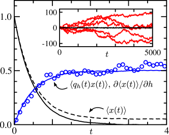
Figure 1: (color online) Numerical simulation of Eqs. (5) with $\kappa=2$, $x_{0}=1$, and $D=T=1$. The falling curves show $\langle x(t)\rangle$ for $h=0$ (solid line) and $h=0.1$ (dashed line). The rising curves show $\langle x(t)q_{h}(t)\rangle$ (blue solid line) and $\partial\langle x(t)\rangle/\partial h$ evaluated using forward finite differencing (blue circles). Averages are over $10^{5}$ replicate simulations. The inset shows the long-time behaviour of individual $x(t)$ and $q_{h}(t)$ trajectories. While $x(t)$ stays close to its equilibrium value (black), $q_{h}(t)$ (five replicates, red) executes a random walk.

To illustrate the method, we turn to a simple example for which analytical results are available: a single particle in a one-dimensional harmonic trap described by a potential $U=\frac{1}{2}\kappa x^{2}-hx$. To make contact with linear response theory, we take the parameter of interest to be the strength of the applied external force $h$. We set the particle mobility to unity so that the diffusion constant $D=T$ where the temperature $T$ is in units of $k_{\mathrm{B}}$. At equilibrium, $P_{\mathrm{eq}}(x)\sim e^{-U/T}$, so that $\partial\ln P_{\mathrm{eq}}/\partial h=(x-\langle x\rangle)/T$ Prost et al. (2009), and the FDT holds: $\partial\langle x\rangle/\partial h=(\langle x^{2}\rangle-\langle x\rangle^{2})/T$. We now apply Malliavin weight sampling to the time-dependent situation in which the particle starts from $x=x_{0}$ at $t=0$ and relaxes towards its equilibrium position. Eqs. (1) and (2) become

$$\frac{d{x}}{dt}=-\kappa x+h+\eta,\quad\frac{d{q_{h}}}{dt}=\frac{\eta}{2T}\,.$$ (5)

These equations can be solved exactly sup to give $P(x,q_{h};t)$ as a bivariate Gaussian with

$$\begin{array}[]{l}\langle x\rangle=x_{0}e^{-\kappa t}+({h}/{\kappa})(1-e^{-\kappa t})\,,\quad\langle q_{h}\rangle=0\,,\\[6.0pt] \langle x^{2}\rangle-\langle x\rangle^{2}=({T}/{\kappa})(1-e^{-2\kappa t})\,,\\[6.0pt] \langle xq_{h}\rangle=({1-e^{-\kappa t}})/{\kappa}\,,\quad\langle q_{h}^{2}\rangle={t}/{2T}\,.\end{array}$$ (6)

This result allows us to verify directly that Eq. (4) is satisfied, that is to say $\langle q_{h}\rangle_{x}=\int\!dx\,q_{h}P(x,q_{h};t)=\partial\ln P(x;t)/\partial h$, where $P(x;t)=\int\!dq_{h}\,P(x,q_{h};t)$. Fig. 1 shows simulation results for $\partial\langle x\rangle/\partial h$, computed by Malliavin weight sampling (MWS) and by forward finite differencing; the inset shows trajectories for $q_{h}$ from replicate simulation runs. The Malliavin weight $q_{h}$ behaves as a random walk with zero mean and a diffusion coefficient $1/4T$. Eq. (6) shows that, by analogy with the equilibrium FDT, one can define a time-dependent effective temperature $T_{\mathrm{eff}}/T=(1-e^{-2\kappa t})/(1-e^{-\kappa t})$ such that $\partial\langle x\rangle/\partial h=(\langle x^{2}\rangle-\langle x\rangle^{2})/T_{\mathrm{eff}}$. Calculating the conditional average of the Malliavin weight gives $\langle q_{h}\rangle_{x}=(x-\langle x\rangle)/T_{\mathrm{eff}}$. Interestingly this has the same form as the equilibrium case but again features $T_{\mathrm{eff}}$. Thus the effective temperature has a wider relevance than would be apparent from the time-dependent FDT since $\partial\langle A\rangle/\partial h=(\langle Ax\rangle-\langle A\rangle\langle x\rangle)/T_{\mathrm{eff}}$, where $A(x)$ is any function of the particle position.

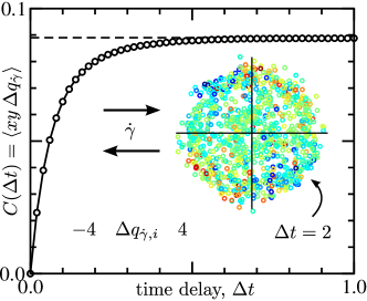
Figure 2: (color online) Interacting particles in a two-dimensional harmonic trap under shear. The main plot shows how the correlation function $\langle xy\Delta q_{\dot{\gamma}}\rangle$ (solid line; calculated in an unsheared system) asymptotes to $\partial\langle xy\rangle/\partial\dot{\gamma}|_{\dot{\gamma}=0}=0.0890\pm 0.0005$ calculated by centered finite differencing (dashed line). The inset shows 100 superimposed simulation snapshots at $\Delta t=2$, colored by individual particle Malliavin weight.

An important practical issue is raised by the fact that $q_{\lambda}(t)$ behaves as a random walk (inset to Figure 1): to compute responses to parameter perturbations for systems in steady state, we cannot simply monitor $q_{\lambda}$ for longer and longer times until the system reaches its steady state. This is because replicate trajectories of $q_{\lambda}$ diverge at long times and measurements of $\langle A(t)q_{\lambda}(t)\rangle$ incur a large sampling error. Fortunately, we can circumvent this problem by computing instead the correlation function Berthier (2007); Warren and Allen (2012) $C(t,t_{0})=\langle A(t)\,\Delta q_{\lambda}(t,t_{0})\rangle$ where $\Delta q_{\lambda}(t,t_{0})=q_{\lambda}(t)-q_{\lambda}(t_{0})$. In steady state this becomes a well-defined function of $\Delta t=t-t_{0}$ and we expect it to obey $C(\Delta t)\to\partial\langle A\rangle/\partial\lambda$ as $\Delta t\to\infty$ Warren and Allen (2012); sup . Like any other correlation function, $C(t)$ converges to its asymptotic value on a time scale set by the spectrum of relaxation times in the problem.

Next, we demonstrate the application of MWS to a much less trivial example: a non-equilibrium driven steady state formed by a cluster of particles in a two-dimensional harmonic trap, under shear. This example is motivated by recent experimental studies of colloidal particles in optical traps, which have provided new insights into statistical physics at the microscale KSG . We suppose that the particles interact with each other via a repulsive screened Coulomb potential $u(r)=(\Gamma/r)e^{-r/r_{c}}$, with coupling strength $\Gamma$ and range $r_{c}$. The total potential energy of the cluster is then $U=\sum_{i>j}u(r_{ij})+\frac{1}{2}\kappa\sum_{i}r_{i}^{2}$ (where $\kappa$ is the spring constant of the trap), and the Langevin equations for the particle positions ($x_{i},y_{i}$) are

$$\frac{d{x_{i}}}{dt}=-\frac{\partial U}{\partial x_{i}}+\dot{\gamma}y_{i}+\eta_{x,i}\,,\quad\frac{d{y_{i}}}{dt}=-\frac{\partial U}{\partial y_{i}}+\eta_{y,i}$$ (7)

where $\dot{\gamma}$ is the shear rate and $\eta_{x,i}$ and $\eta_{y,i}$ are noise terms defined as in the previous example. We set $r_{c}=k_{\mathrm{B}}T=D=1$ to fix units of length, energy, and time, and choose $N=10$, $\kappa=10$ and $\Gamma=25$; for this parameter set, the particles form a dense, strongly correlated cluster in the trap (see inset to Fig. 2). To characterize the morphology of the cluster we use quantities like $\langle xy\rangle\equiv\langle\sum_{i=1}^{N}x_{i}y_{i}\rangle/N$. We first focus on the sensitivity of this quantity to changes in the shear rate $\dot{\gamma}$. We therefore track the Malliavin weight $q_{\dot{\gamma}}$ which, from Eq. (2), obeys

$$\begin{array}[]{l}\displaystyle\frac{d{q_{\dot{\gamma}}}}{dt}=\frac{1}{2k_{\mathrm{B}}T}{\sum_{i=1}^{N}}{y_{i}\eta_{x,i}}\\[6.0pt] \end{array}$$ (8)

To compute $\partial\langle xy\rangle/\partial\dot{\gamma}$ for the system in steady-state, we use the correlation function approach outlined above. Fig. 2 shows that, for $\dot{\gamma}=0$, $C(\Delta t)=\langle(1/N)(\sum_{i=1}^{N}x_{i}(t)y_{i}(t))(q_{\dot{\gamma}}(t)-q_{\dot{\gamma}}(t-\Delta t))\rangle$ tends to $\partial\langle xy\rangle/\partial\dot{\gamma}|_{\dot{\gamma}=0}$ as $\Delta t$ increases, where $\partial\langle xy\rangle/\partial\dot{\gamma}|_{\dot{\gamma}=0}$ (the dashed line) is calculated by finite differencing. In fact the Malliavin weight $q_{\dot{\gamma}}$ turns out to be an interesting physical quantity in itself. By splitting the sum in Eq. (8) into individual particle contributions, one can track Malliavin weights $q_{\dot{\gamma},i}$ for each individual particle. These provide insight into the response to shear of the one-particle probability distribution $P(x_{i},y_{i})$. As shown in the inset to Fig. 2b, the individual contributions to the Malliavin weight are biased towards being positive in the first and third quadrants and negative in the second and fourth quadrants, corresponding to the distortion of the particle cloud by the shear.

An important feature of MWS is that, from a single simulation run, one can compute the sensivitities of any function of the particle coordinates, to any parameter of the system. One simply needs to track the Malliavin weights corresponding to all the parameters that are of interest, using the appropriate dynamical rules as derived from Eq. (2). For example in this problem $q_{\Gamma}$ obeys

$$\begin{array}[]{l}\displaystyle\frac{d{q_{\Gamma}}}{dt}=-\frac{1}{2k_{\mathrm{B}}T}{\sum_{i=1}^{N}}\Bigl{(}\frac{\partial^{2}U}{\partial\Gamma\partial x_{i}}\eta_{x,i}+\frac{\partial^{2}U}{\partial\Gamma\partial y_{i}}\eta_{y,i}\Bigr{)}\,.\end{array}$$ (9)

and an analogous equation for $q_{\kappa}$ is easily written down. Fig. 3a shows the full panoply of responses of the cluster morphology parameters $\langle xy\rangle$ and $\langle x^{2}y^{2}\rangle$ to the parameters of the problem, for $\Gamma=25$, obtained from a single simulation run. Second order derivatives were computed as described in Supplementary Material sup .

We now demonstrate how MWS can reveal subtle details of how the response to shear, $\partial\langle xy\rangle/\partial\dot{\gamma}|_{\dot{\gamma}=0}$, depends on $\langle x^{2}y^{2}\rangle^{1/2}$, which provides a representative measure of the area of the particle cloud. For non-interacting particles one can obtain analytically sup the intriguing quasi-FDT result $\partial\langle xy\rangle/\partial\dot{\gamma}=\langle x^{2}y^{2}\rangle/2T$, which holds at $\Gamma=\dot{\gamma}=0$ and for all values of $\kappa$. The case of interacting particles, however, cannot be solved analytically. We therefore simulated the cloud at a series of increasing values of $\Gamma$ (i. e.  increasing cluster size) keeping $\kappa=10$. The results shown in Fig 3b suggest that $\partial\langle xy\rangle/\partial\dot{\gamma}|_{\dot{\gamma}=0}$ is quite accurately proportional to $\langle x^{2}y^{2}\rangle^{1/2}$. More generally we can define an effective exponent $\beta=d\ln(\partial\langle xy\rangle/\partial\dot{\gamma})/d\ln\langle x^{2}y^{2}\rangle$. This can be evaluated as $\Gamma$ varies at fixed $\kappa$, or vice versa. In the former case, expanding the derivatives gives

$$\beta=\frac{\langle x^{2}y^{2}\rangle}{\partial\langle x^{2}y^{2}\rangle/\partial\Gamma}\times\frac{\partial^{2}\langle xy\rangle/\partial\dot{\gamma}\partial\Gamma}{\partial\langle xy\rangle/\partial\dot{\gamma}}\,.$$ (10)

We used MWS to compute the derivatives in Eq. (10), with results shown in the inset in Fig. 3b. As expected from the main plot, $\beta\approx 0.5$, but a more subtle dependence is also apparent. An analogous calculation for the latter case (fixed $\Gamma$ varying $\kappa$) shows that the corresponding effective exponent increases from $\beta=1$ at $\Gamma=0$ (the quasi-FDT result) to $\beta\approx 1.3$ at $\Gamma=25$. Hence the interacting particle case shows considerably more complexity than the non-interacting one, and there is apparently little universality.

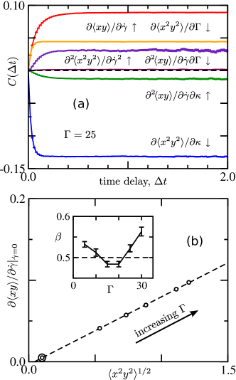
Figure 3: (color online) (a) Multiple parameter dependencies from a single simulation. (b) Dependence of shear response on the size of the cluster, as the interaction strength $\Gamma$ is varied (the double circle is $\Gamma=0$). The inset shows the effective exponent $\beta$ computed from Eq. (10) in the main text, using MWS to evaluate the derivatives.

These examples demonstrate that MWS provides a simple and easy-to-implement alternative to finite differencing, for Brownian dynamics problems that may be time-dependent or in steady state, in or out of equilibrium. Let us now discuss the question of efficiency. As highlighted above, in MWS one has access to response coefficients for all parameters of the problem (for which the derivatives $\partial{\vec{f}}_{i}/\partial\lambda$ in Eq. (2) are known), with little additional cost, since integrating the equations of motion for the $q_{\lambda}$ requires no new random numbers and also typically does not require recalculation of the forces. MWS also scales more efficiently with the computational effort than does standard finite differencing. For MWS, the error in a computation of $\partial\langle A(t)\rangle/\partial\lambda$ scales as $M^{-1/2}$, where $M$ is the number of replicate simulation runs used to compute the averages (this follows from the usual scaling of the standard error in the mean with the number of samples). For finite differencing, there is an inherent tradeoff between the systematic error introduced by using a too-large perturbation and the random sampling error that arises when the perturbation is very small. One can show L’Ecuyer (1992) that the best possible choice of the perturbation size results in an error that scales as $M^{-1/4}$ for a forward finite differencing scheme, and $M^{-1/3}$ for a centered scheme. Although the scaling can be improved to $M^{-1/2}$ by using a common random number scheme L’Ecuyer (1992); Rathinam et al. (2010), even here we expect MWS to be more efficient, since it does not require the perturbed system to be explicitly simulated. For example we note that more than six times as many force evaluations were used to calculate $\partial\langle xy\rangle/\partial\dot{\gamma}$ in Fig. 2 by finite differencing, compared to calculating the same quantity to comparable accuracy by the MWS correlation function method.

MWS has the potential greatly to facilitate the parameterization of force fields, when combined with gradient-based search and optimisation algorithms. This should be especially relevant for mesoscale problems where Brownian dynamics algorithms such as dissipative particle dynamics (DPD) are often the method of choice Frenkel and Smit (2002) (note that the application to DPD should take account of the fact that the noise terms are pairwise central random forces). An equally important application of MWS is in the computation of response functions to external fields—for example in the context of dynamical phase transitions. Interestingly, while we have focused here only on its long-time limit, the time-correlation function $C(\Delta t)$ is actually equivalent to the time-dependent response to a step perturbation. This point will be explored in more detail in future work. A particularly interesting question concerns the extent to which the Malliavin weight itself can be used as an autonomous order parameter. For instance in the 1d trap problem the conditional average $\langle q_{h}\rangle_{x}$ features the time-dependent effective temperature $T_{\mathrm{eff}}$, generalising the linear response result. Certainly for glassy systems we expect that the correlation functions $\langle A\,\Delta q_{\lambda}\rangle$ will show typical non-ergodic memory and aging phenomenology Berthier (2007): it is interesting to speculate whether the behaviour of $q_{\lambda}$ itself could be used as an alternative signature of glassy behaviour.

We thank Mike Allen, Mike Cates, Alessandro Laio and Bartlomiej Waclaw for discussions. RJA is supported by a Royal Society University Research Fellowship and by EPSRC under grants EP/I030298/1 and EP/EO30173.

SUPPLEMENTARY MATERIAL

S0.1 Proof of Eqs. (3) and (4) in the main text

We start by introducing the probability distribution $P(\{{\vec{r}}_{i}\};t)$ for the particle positions, and the joint probability distribution $P(\{{\vec{r}}_{i}\},q_{\lambda};t)$ for the combination of the particle positions and the Malliavin weight. The two are related by

$$\textstyle P(\{{\vec{r}}_{i}\};t)=\int\!dq_{\lambda}\,P(\{{\vec{r}}_{i}\},q_{\lambda};t)\,.$$ (S1)

We also define the conjugate variable

$$Q_{\lambda}(\{{\vec{r}}_{i}\};t)\equiv\frac{\partial\ln P(\{{\vec{r}}_{i}\};t)}{\partial\lambda}=\frac{1}{P(\{{\vec{r}}_{i}\};t)}\frac{\partial P(\{{\vec{r}}_{i}\};t)}{\partial\lambda}\,,$$ (S2)

and the conditional average

$$\langle q_{\lambda}\rangle_{\{{\vec{r}}_{i}\}}\equiv\frac{\int\!dq_{\lambda}\,q_{\lambda}\,P(\{{\vec{r}}_{i}\},q_{\lambda};t)}{\int\!dq_{\lambda}\,P(\{{\vec{r}}_{i}\},q_{\lambda};t)}\,.$$ (S3)

The first goal is to show the equivalence of $Q_{\lambda}$ and $\langle q_{\lambda}\rangle_{\{{\vec{r}}_{i}\}}$—Eq. (4) in the main text. We do this by showing that they both obey the same evolution equation.

As hinted at in the main text, we introduce an explicit Euler-type scheme for updating the particle positions. This also makes explicit the updating rule associated with the Malliavin weight. We therefore write

$${\vec{r}}_{i}{}^{\prime}={\vec{r}}_{i}+\frac{D{\vec{f}}_{i}\delta t}{k_{\mathrm{B}}T}+{\vec{\xi}}_{i}$$ (S4)

where ${\vec{r}}_{i}{}^{\prime}$ is the updated position of the $i$th particle at time $t+\delta t$, $\delta t$ is the time step, and the ${\vec{\xi}}_{i}$ are a set of $3N$ Gaussian random variates of zero mean and variance $2D\delta t$. The corresponding updating rule for the Malliavin weight is

$$q_{\lambda}^{\prime}=q_{\lambda}+\frac{1}{2k_{\mathrm{B}}T}\sum_{i=1}^{N}\frac{\partial{\vec{f}}_{i}}{\partial\lambda}\cdot{\vec{\xi}}_{i}\,.$$ (S5)

Note that the exact same sequence of random variates ${\vec{\xi}}_{i}$ is used for updating the particle positions and the Malliavin weight. In this Euler scheme $P(\{{\vec{r}}_{i}\};t)$ obeys a Chapman-Kolmogorov equation

$$\begin{array}[]{l}P(\{{\vec{r}}_{i}{}^{\prime}\};t+\delta t)={\textstyle\int\prod_{i}d^{3}{\vec{r}}_{i}}\,P(\{{\vec{r}}_{i}\};t)\\[6.0pt] {}\hskip 120.00018pt\,\times W(\{{\vec{r}}_{i}{}^{\prime}\}|\{{\vec{r}}_{i}\})\end{array}$$ (S6)

where the propagator is

$$W(\{{\vec{r}}_{i}{}^{\prime}\}|\{{\vec{r}}_{i}\})={({4\pi D\,\delta t})^{-3N/2}}\exp\Bigl{(}-\frac{\sum_{i=1}^{N}({\vec{r}}_{i}{}^{\prime}-{\vec{r}}_{i}-D{\vec{f}}_{i}\delta t/k_{\mathrm{B}}T)^{2}}{4D\,\delta t}\Bigr{)}\,.$$ (S7)

Differentiating the Chapman-Kolmogorov equation with respect to $\lambda$ leads to an adjunct equation for the conjugate variable $Q_{\lambda}$,

$$Q_{\lambda}(\{{\vec{r}}_{i}{}^{\prime}\};t+\delta t)\,P(\{{\vec{r}}_{i}{}^{\prime}\};t+\delta t)=\int\prod_{i}d^{3}{\vec{r}}_{i}\,\Bigl{[}Q_{\lambda}(\{{\vec{r}}_{i}\};t)+\frac{\partial\ln W}{\partial\lambda}\Bigr{]}\,P(\{{\vec{r}}_{i}\};t)\,W(\{{\vec{r}}_{i}{}^{\prime}\}|\{{\vec{r}}_{i}\})\,.$$ (S8)

The second quantity in the square brackets in Eq. (S8) is

$$\frac{\partial\ln W}{\partial\lambda}\equiv\frac{\partial\ln W(\{{\vec{r}}_{i}{}^{\prime}\}|\{{\vec{r}}_{i}\})}{\partial\lambda}=\frac{1}{2k_{\mathrm{B}}T}\sum_{i=1}^{N}\frac{\partial{\vec{f}}_{i}}{\partial\lambda}\cdot\Bigl{(}{\vec{r}}_{i}{}^{\prime}-{\vec{r}}_{i}-\frac{D{\vec{f}}_{i}\delta t}{k_{\mathrm{B}}T}\Bigr{)}\,.$$ (S9)

We now show that Eq. (S8) for the evolution of $Q_{\lambda}$ is replicated by the evolution equation for the Malliavin weight. The joint probability distribution function $P(\{{\vec{r}}_{i}\},q_{\lambda};t)$ obeys an extended Chapman-Kolmogorov equation

$$P(\{{\vec{r}}_{i}{}^{\prime}\},q_{\lambda}^{\prime};t+\delta t)=\int\prod_{i}d^{3}{\vec{r}}_{i}\,d^{3}{\vec{\xi}}_{i}\,\,dq_{\lambda}\,P(\{{\vec{r}}_{i}\},q_{\lambda};t)\,P(\{{\vec{\xi}}_{i}\})\,\delta({\vec{r}}_{i}{}^{\prime}-{\vec{r}}_{i}-\Delta_{i})\,\delta(q_{\lambda}^{\prime}-q_{\lambda}-\Delta_{q})$$ (S10)

where

$$\Delta_{i}({\vec{r}}_{i},{\vec{\xi}}_{i})=\frac{D{\vec{f}}_{i}\delta t}{k_{\mathrm{B}}T}+{\vec{\xi}}_{i}\,,\qquad\Delta_{q}({\vec{r}}_{i},{\vec{\xi}}_{i})=\frac{1}{2k_{\mathrm{B}}T}\sum_{i=1}^{N}\frac{\partial{\vec{f}}_{i}}{\partial\lambda}\cdot{\vec{\xi}}_{i}$$ (S11)

give the discrete increments to the particle positions and Malliavin weight. The two $\delta$-functions in Eq. (S10) enforce these updating rules. The function $P(\{{\vec{\xi}}_{i}\})$ is a $3N$-dimensional Gaussian. The $3N$ random variates ${\vec{\xi}}_{i}$ are uncorrelated and have zero mean and variance $2D\delta t$. With the definitions in Eqs. (S2) and (S3) in hand we take the first moment of Eq. (S10) with respect to $q_{\lambda}$ to get

$$\textstyle\langle q_{\lambda}\rangle_{\{{\vec{r}}_{i}{}^{\prime}\},t+\delta t}\,P(\{{\vec{r}}_{i}{}^{\prime}\};t+\delta t)=\int\!dq_{\lambda}^{\prime}\,q_{\lambda}^{\prime}\,P(\{{\vec{r}}_{i}{}^{\prime}\},q_{\lambda}^{\prime};t+\delta t)$$ (S12a)

$$\textstyle{}\quad=\int\prod_{i}d^{3}{\vec{r}}_{i}\,d^{3}{\vec{\xi}}_{i}\,dq_{\lambda}\,dq_{\lambda}^{\prime}\,q_{\lambda}^{\prime}\,P(\{{\vec{r}}_{i}\},q_{\lambda};t)\,P(\{{\vec{\xi}}_{i}\})\,\delta({\vec{r}}_{i}{}^{\prime}-{\vec{r}}_{i}-\Delta_{i})\,\delta(q_{\lambda}^{\prime}-q_{\lambda}-\Delta_{q})$$ (S12b)

$$\textstyle{}\quad=\int\prod_{i}d^{3}{\vec{r}}_{i}\,d^{3}{\vec{\xi}}_{i}\,dq_{\lambda}\,[q_{\lambda}+\Delta_{q}]\,P(\{{\vec{r}}_{i}\},q_{\lambda};t)\,P(\{{\vec{\xi}}_{i}\})\,\delta({\vec{r}}_{i}{}^{\prime}-{\vec{r}}_{i}-\Delta_{i})$$ (S12c)

$$\textstyle{}\quad=\int\prod_{i}d^{3}{\vec{r}}_{i}\,dq_{\lambda}\,[q_{\lambda}+\Delta_{q}]\,P(\{{\vec{r}}_{i}\},q_{\lambda};t)\,W(\{{\vec{r}}_{i}{}^{\prime}\}|\{{\vec{r}}_{i}\})$$ (S12d)

$$\textstyle{}\quad=\int\prod_{i}d^{3}{\vec{r}}_{i}\,[\langle q_{\lambda}\rangle_{\{{\vec{r}}_{i}\}}+\Delta_{q}]\,P(\{{\vec{r}}_{i}\};t)\,W(\{{\vec{r}}_{i}{}^{\prime}\}|\{{\vec{r}}_{i}\})\,.$$ (S12e)

To progress from Eq. (S12b) to (S12e) we do successively the $q_{\lambda}^{\prime}$ integral, the ${\vec{\xi}}_{i}$ integrals, and the $q_{\lambda}$ integral; using first the $\delta$-functions then the definition of the conditional average for the final step. In doing the ${\vec{\xi}}_{i}$ integrations, we recover the propagator $W({\vec{r}}_{i}{}^{\prime}|{\vec{r}}_{i})$ given by Eq. (S7) and the $q_{\lambda}$ increment becomes

$$\Delta_{q}({\vec{r}}_{i},{\vec{r}}_{i}{}^{\prime})=\frac{1}{2k_{\mathrm{B}}T}\sum_{i=1}^{N}\frac{\partial{\vec{f}}_{i}}{\partial\lambda}\cdot\Bigl{(}{\vec{r}}_{i}{}^{\prime}-{\vec{r}}_{i}-\frac{D{\vec{f}}_{i}\delta t}{k_{\mathrm{B}}T}\Bigr{)}\,.$$ (S13)

This is identical to Eq. (S9) therefore we conclude that Eq. (S12e) for updating $\langle q_{\lambda}\rangle_{{\vec{r}}_{i}}$ is identical to Eq. (S8) for updating the conjugate variable $Q_{\lambda}$. By choice these two quantities can be given the same initial values, thus establishing their equivalence, in other words

$$\frac{\int\!dq_{\lambda}\,q_{\lambda}\,P(\{{\vec{r}}_{i}\},q_{\lambda};t)}{\int\!dq_{\lambda}\,P(\{{\vec{r}}_{i}\},q_{\lambda};t)}=\frac{\partial\ln P(\{{\vec{r}}_{i}\};t)}{\partial\lambda}\,.$$ (S14)

To establish Eq. (3) in the main text we use Eq. (S1) and the second half of Eq. (S2) to rearrange Eq. (S14) into the alternative form $\int\!dq_{\lambda}\,q_{\lambda}\,P(\{{\vec{r}}_{i}\},q_{\lambda};t)={\partial P(\{{\vec{r}}_{i}\};t)}/{\partial\lambda}$. Eq. (3) follows from this since

$$\begin{array}[]{l}\langle Aq_{\lambda}\rangle=\int\prod_{i}d^{3}{\vec{r}}_{i}\,dq_{\lambda}\,A(\{{\vec{r}}_{i}\})\,q_{\lambda}\,P(\{{\vec{r}}_{i}\},q_{\lambda};t)\\[12.0pt] \displaystyle{}\hskip 40.00006pt={\textstyle\int\prod_{i}d^{3}{\vec{r}}_{i}}\,A(\{{\vec{r}}_{i}\})\,\frac{\partial P(\{{\vec{r}}_{i}\};t)}{\partial\lambda}=\frac{\partial({\textstyle\int\prod_{i}d^{3}{\vec{r}}_{i}}\,A(\{{\vec{r}}_{i}\})\,P(\{{\vec{r}}_{i}\};t))}{\partial\lambda}=\frac{\partial\langle A\rangle}{\partial\lambda}\,.\end{array}$$ (S15)

S0.2 Practical implementation

The implementation of MWS in a Brownian dynamics code is quite straightforward. The main point is that for efficiency one may want to update the Malliavin weight(s) according to Eq. (S5) at the same time as calculating the forces. This requires that the set of random variates ${\vec{\xi}}_{i}$ be computed and stored at the start of the step, as in the following schematic algorithm :

• generate the $3N$ random variates ${\vec{\xi}}_{i}$,

• compute the forces ${\vec{f}}_{i}(\{{\vec{r}}_{i}\})$ and the quantity $\sum_{i=1}^{N}(\partial{\vec{f}}_{i}/\partial\lambda)\cdot{\vec{\xi}}_{i}$,

• update the particle positions according in Eq. (S4),

• update the Malliavin weight(s) according in Eq. (S5),

• record any quantities of interest, i. e. $A(\{{\vec{r}}_{i}\})$, and the value of the Malliavin weight(s).

The last item does not necessarily have to be done every time step of course. As indicated in the main text, the algorithm is initialised by setting the particle positions to their initial values and the Malliavin weights to zero. For steady state problems there are two approaches to the use of the MWS correlation function method. The simplest is to choose a set of equally spaced reference points $t_{0}=nT$ for the calculation of $\Delta q_{\lambda}=q_{\lambda}(t)-q_{\lambda}(t_{0})$, where $T$ is a time period longer than the expected relaxation time of the system (which may have to be determined by trial and error). In this approach, every $n$ timesteps the current values of $q_{\lambda}(t)$ and $A(t)$ are recorded. The running value of $q_{\lambda}$ is then set to zero and the simulation continued. The time average of the stored values of $q_{\lambda}A$ gives $\partial\langle A\rangle/\partial\lambda$. More efficient is to use a sliding window to calculate the correlation function. Block averaging can be used for error estimates.

S0.3 Underdamped Brownian dynamics

The extension of MWS to underdamped Brownian dynamics is fairly simple. We denote the particle positions by ${\vec{r}}_{i}$ and velocities by ${\vec{v}}_{i}$. The dynamical equations are

$$\frac{d{{\vec{r}}_{i}}}{dt}={\vec{v}}_{i}\,,\quad m\frac{d{{\vec{v}}_{i}}}{dt}={\vec{f}}_{i}-\gamma{\vec{v}}_{i}+{\vec{\eta}}_{i}$$ (S16)

where $m$ is the mass, $\gamma$ is the frictional drag coefficient, and ${\vec{\eta}}_{i}$ are white noise terms of amplitude $2\gamma k_{\mathrm{B}}T$. An Euler-type scheme for Eqs. (S16) is

$${\vec{r}}_{i}{}^{\prime}={\vec{r}}_{i}+{\vec{v}}_{i}\delta t\,\,\quad{\vec{v}}_{i}{}^{\prime}={\vec{v}}_{i}+\frac{({\vec{f}}_{i}-\gamma{\vec{v}}_{i})\delta t}{m}+{\vec{\xi}}_{i}$$ (S17)

where the ${\vec{\xi}}_{i}$ are 3N Gaussian random variates of zero mean and variance $2\gamma k_{\mathrm{B}}T\,\delta t/m^{2}$ (note that we divided the velocity equations through by $m$). It follows that the probability distribution function $P(\{{\vec{r}}_{i}\},\{{\vec{v}}_{i}\};t)$ evolves according to the Chapman-Kolmogorov equation

$$P(\{{\vec{r}}_{i}{}^{\prime}\},\{{\vec{v}}_{i}{}^{\prime}\};t+\delta t)=\int\prod_{i}d^{3}{\vec{r}}_{i}\,d^{3}{\vec{v}}_{i}\,P(\{{\vec{r}}_{i}\},\{{\vec{v}}_{i}\};t)\,\delta({\vec{r}}_{i}{}^{\prime}-{\vec{r}}_{i}-{\vec{v}}_{i}\delta t)\,W(\{{\vec{v}}_{i}{}^{\prime}\}|\{{\vec{v}}_{i}\},\{{\vec{r}}_{i}\})$$ (S18)

where the partial propagator is

$$W(\{{\vec{v}}_{i}{}^{\prime}\}|\{{\vec{v}}_{i}\},{\vec{r}}_{i})=(4\pi\gamma k_{\mathrm{B}}T\,\delta t/m^{2})^{-3N/2}\exp\Bigl{(}-\frac{\sum_{i=1}^{N}({\vec{v}}_{i}{}^{\prime}-{\vec{v}}_{i}-({\vec{f}}_{i}-\gamma{\vec{v}}_{i})\delta t/m)^{2}}{4\gamma k_{\mathrm{B}}T\,\delta t/m^{2}}\Bigr{)}\,.$$ (S19)

If we differentiate Eq. (S18) with respect to some parameter $\lambda$ we obtain

$$\begin{array}[]{l}Q_{\lambda}(\{{\vec{r}}_{i}{}^{\prime}\},\{{\vec{v}}_{i}{}^{\prime}\};t+\delta t)\,P(\{{\vec{r}}_{i}{}^{\prime}\},\{{\vec{v}}_{i}{}^{\prime}\};t+\delta t)\\[6.0pt] {}\hskip 60.00009pt=\int\prod_{i}d^{3}{\vec{r}}_{i}\,d^{3}{\vec{v}}_{i}[Q_{\lambda}(\{{\vec{r}}_{i}\},\{{\vec{v}}_{i}\};t)+{\partial\ln W}/{\partial\lambda}]\\[6.0pt] {}\hskip 120.00018pt\times\delta({\vec{r}}_{i}{}^{\prime}-{\vec{r}}_{i}-{\vec{v}}_{i}\delta t)\,W(\{{\vec{v}}_{i}{}^{\prime}\}|\{{\vec{v}}_{i}\},\{{\vec{r}}_{i}{}^{\prime}\})\,P(\{{\vec{r}}_{i}\},\{{\vec{v}}_{i}\};t)\end{array}$$ (S20)

where $Q_{\lambda}(\{{\vec{r}}_{i}\},\{{\vec{v}}_{i}\};t)\equiv\partial\ln P(\{{\vec{r}}_{i}\},\{{\vec{v}}_{i}\};t)/\partial\lambda$. This again suggests the updating rule for the Malliavin weight, $q_{\lambda}^{\prime}=q_{\lambda}+\partial\ln W/\partial\lambda$, in other words the derivation is impervious to the presence of a $\delta$-function in the full propagator. Inserting the explicit expression for $W$, and assuming the parameter of interest features only in the force law, gives the Langevin equation

$$\frac{d{q_{\lambda}}}{dt}=\frac{m}{2\gamma k_{\mathrm{B}}T}\sum_{i=1}^{N}\frac{\partial{\vec{f}}_{i}}{\partial\lambda}\cdot{\vec{\eta}}_{i}\,.$$ (S21)

This result is very similar to the overdamped case. As a demonstration let us revisit the example of Brownian motion in a one-dimensional trap, but this time consider the underdamped case. The Langevin equations are

$$\frac{d{x}}{dt}=v,\quad m\frac{d{v}}{dt}=-\gamma v-\kappa x+h+\eta,$$ (S22)

and

$$\frac{d{q_{h}}}{dt}=\frac{m\eta}{2\gamma T}\,.$$ (S23)

Fig. S1 shows simulation results confirming that $\langle q_{h}x\rangle=\partial\langle x\rangle/\partial h$.

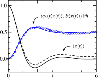
Figure S1: (color) Numerical simulation of Eqs. (S22) and  (S23) with $\kappa=2$, $m=1/2$, $x_{0}=1$, and $\gamma=T=1$. The falling curves show $\langle x(t)\rangle$ for $h=0$ (solid line) and $h=0.1$ (dashed line). The rising curves show $\langle x(t)q_{h}(t)\rangle$ (blue solid line) and $\partial\langle x(t)\rangle/\partial h$ evaluated using forward finite differencing (blue circles). Averages are over $10^{5}$ replicate simulations; cf. Fig. 1 in the main text.

S0.4 Higher-order derivatives

We next demonstrate how MWS extends to the computation of higher-order derivatives. A double application of Eq. (3) in the main text, for two parameters $\lambda$ and $\mu$, gives

$$\frac{\partial^{2}\!\langle A(\{{\vec{r}}_{i}\})\rangle}{\partial\lambda\partial\mu}=\langle A(\{{\vec{r}}_{i}\})\,(q_{\lambda\mu}+q_{\lambda}q_{\mu})\rangle$$ (S24)

where $q_{\lambda\mu}=\partial q_{\lambda}/\partial\mu$. Differentiating the discrete updating rule $q_{\lambda}^{\prime}=q_{\lambda}+\partial\ln W/\partial\lambda$ with respect to $\mu$ gives $q_{\lambda\mu}^{\prime}=q_{\lambda\mu}+\partial^{2}\!\ln W/\partial\lambda\partial\mu$. We insert the expression for $W$ from Eq. (S7) into this, and simplify, to find the corresponding Langevin equation

$$\frac{d{q_{\lambda\mu}}}{dt}=\frac{1}{2k_{\mathrm{B}}T}\sum_{i=1}^{N}\Bigl{[}\frac{\partial^{2}\!{\vec{f}}_{i}}{\partial\lambda\partial\mu}\cdot{\vec{\eta}}_{i}-\frac{D}{k_{\mathrm{B}}T}\frac{\partial{\vec{f}}_{i}}{\partial\lambda}\cdot\frac{\partial{\vec{f}}_{i}}{\partial\mu}\Bigr{]}\,.$$ (S25)

The new feature in this is a drift term (the last term) which has the consequence that $\langle q_{\lambda\mu}\rangle=-\langle q_{\lambda}q_{\mu}\rangle$. This ensures that ${\partial^{2}\!\langle A\rangle}/{\partial\lambda\partial\mu}=0$ if $A$ is a constant.

Note that, as a result of the peculiar properties of the stochastic differential calculus, Eq. (S25) is not simply found by differentiating Eq. (2) in the main text; rather one has to proceed via the discrete updating rules. Also note that the second-order Malliavin weight $q_{\lambda\mu}$ defined in Eq. (S25) must be combined with the two first-order Malliavin weights $q_{\lambda}$ and $q_{\mu}$ to obtain the correct weighted average in Eq. (S24). We have tested the second-order MWS scheme for the trapped interacting particle cloud under shear, see for example Fig 3a in the main text.

S0.5 One-dimensional trap

Here we derive the expressions in Eqs. (6) for the transient behaviour of a particle in a one-dimensional harmonic trap. Eqs. (5) in the main text are

$$\frac{d{x}}{dt}=-\kappa x+h+\eta,\quad\frac{d{q_{h}}}{dt}=\frac{\eta}{2T}\,.$$ (S26)

These can be integrated to find

$$\begin{array}[]{l}\displaystyle x(t)=x_{0}e^{-\kappa t}+\frac{h}{\kappa}(1-e^{-\kappa t})+\int_{0}^{t}\!dt^{\prime}\,e^{-\kappa(t-t^{\prime})}\eta(t^{\prime})\,,\\[12.0pt] \displaystyle q_{h}(t)=\frac{1}{2T}\int_{0}^{t}\!dt^{\prime}\,\eta(t^{\prime})\,.\end{array}$$ (S27)

Since $x$ and $q_{h}$ are summed Gaussian random noises, it follows that $P(x,q_{h};t)$ is a Gaussian—cf. §3.5.2 in The Theory of Polymer Dynamics M. Doi and S. F. Edwards (OUP, 1986). To characterise this Gaussian, it suffices to calculate the first and second moments. The first moments follow immediately from Eqs. (S27) and are $\langle x\rangle=x_{0}e^{-\kappa t}+({h}/{\kappa})(1-e^{-\kappa t})$ and $\langle q_{h}\rangle=0$, as given in the first line of Eqs. (6). Therefore $x-\langle x\rangle=\int_{0}^{t}\!dt^{\prime}\,e^{-\kappa(t-t^{\prime})}\eta(t^{\prime})$. The second moment of $x$ (the second line of Eqs. (6)) is

$$\langle x^{2}\rangle-\langle x\rangle^{2}=\int_{0}^{t}\!dt^{\prime}\!\int_{0}^{t}\!dt^{\prime\prime}\,e^{-\kappa(t-t^{\prime})}\,e^{-\kappa(t-t^{\prime\prime})}\times 2T\,\delta(t^{\prime}-t^{\prime\prime})=\frac{T}{\kappa}(1-e^{-2\kappa t})$$ (S28)

where we have used $\langle\eta(t^{\prime})\eta(t^{\prime\prime})\rangle=2T\,\delta(t^{\prime}-t^{\prime\prime})$. Likewise the cross correlation term and the second moment of $q_{h}$ (the third line of Eqs. (6)) are

$$\begin{array}[]{l}\displaystyle\langle xq_{h}\rangle=\frac{1}{2T}\int_{0}^{t}\!dt^{\prime}\!\int_{0}^{t}\!dt^{\prime\prime}\,e^{-\kappa(t-t^{\prime})}\times 2T\,\delta(t^{\prime}-t^{\prime\prime})=\frac{1}{\kappa}(1-e^{-\kappa t})\\[12.0pt] \displaystyle\langle q_{h}^{2}\rangle=\frac{1}{(2T)^{2}}\int_{0}^{t}\!dt^{\prime}\!\int_{0}^{t}\!dt^{\prime\prime}\,\times 2T\,\delta(t^{\prime}-t^{\prime\prime})=\frac{t}{2T}\end{array}$$ (S29)

S0.6 Two-dimensional trap in shear

The quasi-FDT result in the main text follows from the steady state probability distribution $P_{\mathrm{ss}}(x,y)$ for a particle in a two-dimensional trap under shear, which can be solved in closed form. Let us recall the Langevin equations for this problem,

$$\frac{d{x}}{dt}=-\kappa x+\dot{\gamma}y+\eta_{x},\quad\frac{d{y}}{dt}=-\kappa y+\eta_{y}\,,$$ (S30)

where $\kappa$ is the trap strength and $\dot{\gamma}$ is the shear rate. In common with the main text we set the particle mobility to unity and write temperature in terms of Boltzmann’s constant, so that we can write $D=T$ for the diffusion coefficient.

From the Smoluchowski equation, the steady-state distribution function corresponding to these Langevin equations satisfies

$$\frac{\partial J_{x}}{\partial x}+\frac{\partial J_{y}}{\partial y}=0$$ (S31)

where the components of the probability current (flux) are

$$\begin{array}[]{l}\displaystyle J_{x}=(-\kappa x+\dot{\gamma}y)P_{\mathrm{ss}}-T\frac{\partial P_{\mathrm{ss}}}{\partial x},\\[12.0pt] \displaystyle J_{y}=-\kappa yP_{\mathrm{ss}}-T\frac{\partial P_{\mathrm{ss}}}{\partial y}\,.\end{array}$$ (S32)

Since the Langevin equations are linear, we expect that $P_{\mathrm{ss}}$ will be a bivariate Gaussian so we write

$$\textstyle P_{\mathrm{ss}}\sim\exp(-\frac{1}{2}Ax^{2}-\frac{1}{2}By^{2}-Cxy)$$ (S33)

where $A$, $B$ and $C$ are coefficients, to be determined. The simplest way to proceed is to insert this as an ansatz into Eqs. (S31) and (S32), to find that the coefficients have to satisfy

$$\begin{array}[]{l}2\kappa=(A+B)T,\\[3.0pt] A\kappa=(A^{2}+C^{2})T,\\[3.0pt] B\kappa=C\dot{\gamma}+(B^{2}+C^{2})T,\\[3.0pt] C\kappa=A\dot{\gamma}/2+(A+B)CT.\end{array}$$ (S34)

These four conditions arise from equating to zero the constant term and the coefficients of $x^{2}$, $y^{2}$ and $xy$ in Eq. (S31). Although there are only three unknowns, Eqs. (S34) are interdependent and admit the unique solution,

$$\begin{array}[]{l}\displaystyle A=\frac{4\kappa^{3}}{({\dot{\gamma}}^{2}+4\kappa^{2})T}\,,\quad B=\frac{4\kappa^{3}+2\kappa\dot{\gamma}^{2}}{({\dot{\gamma}}^{2}+4\kappa^{2})T}\,,\\[12.0pt] \displaystyle C=-\frac{2{\dot{\gamma}}\kappa^{2}}{({\dot{\gamma}}^{2}+4\kappa^{2})T}\,.\end{array}$$ (S35)

Hence the complete steady state distribution function is

$$\begin{array}[]{l}\displaystyle P_{\mathrm{ss}}=\frac{\kappa^{2}}{\pi T\sqrt{\dot{\gamma}^{2}+4\kappa^{2}}}\\[12.0pt] \displaystyle{}\hskip 10.00002pt\times\exp\Bigl{[}-\frac{2\kappa^{3}x^{2}+(2\kappa^{3}+\kappa\dot{\gamma}^{2})y^{2}-2\dot{\gamma}\kappa^{2}xy}{(\dot{\gamma}^{2}+4\kappa^{2})T}\Bigr{]}\,.\end{array}$$ (S36)

For reference, the associated moments are

$$\begin{array}[]{l}\displaystyle\langle x^{2}\rangle_{\mathrm{ss}}=\frac{T}{\kappa}\Bigl{(}1+\frac{\dot{\gamma}^{2}}{2\kappa^{2}}\Bigr{)}\,,\quad\langle y^{2}\rangle_{\mathrm{ss}}=\frac{T}{\kappa}\,,\\[12.0pt] \displaystyle\langle xy\rangle_{\mathrm{ss}}=\frac{\dot{\gamma}T}{2\kappa^{2}}\,.\end{array}$$ (S37)

Differentiating the steady state distribution with respect to the shear rate yields

$$\begin{array}[]{l}\displaystyle\langle q_{\dot{\gamma}}\rangle_{xy}=\frac{\partial\ln P_{\mathrm{ss}}}{\partial\dot{\gamma}}\\[12.0pt] \displaystyle{}\hskip 20.00003pt=\frac{2\kappa^{2}(2\kappa x-\dot{\gamma}y)(\dot{\gamma}x+2\kappa y)}{(\dot{\gamma}^{2}+4\kappa^{2})^{2}T}-\frac{\dot{\gamma}}{\dot{\gamma}^{2}+4\kappa^{2}}\,.\end{array}$$ (S38)

In the limit $\dot{\gamma}\to 0$ this reduces to $\langle q_{\dot{\gamma}}\rangle_{xy}=xy/2T$. An immediate application of this is to deduce the quasi-FDT result in the main text:

$$\frac{\partial\langle xy\rangle}{\partial\dot{\gamma}}\Big{|}_{\dot{\gamma}=0}=\frac{\langle x^{2}y^{2}\rangle}{2T}\,.$$ (S39)

References

Chaikin and Lubensky (1995)
P. M. Chaikin and
T. C. Lubensky,
Principles of condensed matter physics
(CUP, Cambridge,
1995).
Hänggi and Thomas (1982)
P. Hänggi and
H. Thomas,
Phys. Rep. 88,
207 (1982).
Cugliando et al. (1994)
L. F. Cugliando,
J. Kurchan, and
G. Parisi,
J. Phys. I (France) 4,
1641 (1994).
Prost et al. (2009)
J. Prost,
J.-F. Joanny,
and J. M. R.
Parrondo, Phys. Rev. Lett.
103, 090601
(2009).
Ciccotti and Jacucci (1975)
G. Ciccotti and
G. Jacucci,
Phys. Rev. Lett. 35,
789 (1975).
L’Ecuyer (1992)
P. L’Ecuyer,
Ann. Oper. Res. 39,
121 (1992).
Rathinam et al. (2010)
M. Rathinam,
P. W. Sheppard,
and M. Khammash,
J. Chem. Phys. 132,
034103 (2010).
(8)
D. Nualart,
The Malliavin calculus and related topics
(Springer-Verlag, New York,
2006); D. R.
Bell, The Malliavin Calculus
(Dover, Mineola, New York,
2006).
(9)
E. Fournié
et al., Finance Stochast. 3,
391 (1999); for an approach similar in
spirit to the present one see
N. Chen and
P. Glasserman,
Stoch. Proc. Appl. 117,
1689 (2007).
Berthier (2007)
L. Berthier,
Phys. Rev. Lett. 98,
220601 (2007).
Plyasunov and Arkin (2007)
A. Plyasunov and
A. P. Arkin,
J. Comp. Phys. 221,
724 (2007).
Warren and Allen (2012)
P. B. Warren and
R. J. Allen,
J. Chem. Phys. 136,
104106 (2012).
EM (7)
D. L. Ermak
and J. A.
McCammon, J. Chem. Phys.
69, 1352 (1978);
M. P. Allen and
D. J. Tildesley,
Computer simulation of liquids
(Clarendon, Oxford, UK,
1987).
(14)
As an alternative approach one can describe the Langevin
dynamics as a hopping problem in -dimensional configuration space, using
a master equation with a constant total hopping rate. Computation of
sensitivity coefficients and response functions in master equation problems
has been studied by Plyasunov and Arkin using the Girsanov measure transform
Plyasunov and Arkin (2007), by ourselves using the notion of trajectory weights Warren and Allen (2012);
and by Berthier in the context of Monte-Carlo simulations Berthier (2007).
(15)
P. T. Korda,
G. C. Spalding,
and D. G. Grier,
Phys. Rev. B 66,
024504 (2002);
D. M. Carberry et al. Phys. Rev. Lett. 92,
140601 (2004);
Y. Roichman,
B. Sun,
A. Stolarski,
and D. G. Grier,
Phys. Rev. Lett. 101,
128301 (2008);
M. Khan and
A. K. Sood,
EPL 94, 60003
(2011).
Frenkel and Smit (2002)
D. Frenkel and
B. Smit,
Understanding Molecular Simulation: from
Algorithms to Applications (Academic,
San Diego, California, 2002),
2nd ed.
(17)
See Supplementary Material below for the proof of
Eqs. (3) and (4) and implementation notes, the
extension to underdamped Brownian motion and higher-order derivatives, the
derivation of Eqs. (6), and the derivation of the quasi-FDT
result for non-interacting particles in a two-dimensional trap in shear.