Accurate measurement of Cn2 profile with Shack-Hartmann data

Abstract

The precise reconstruction of the turbulent volume is a key point in the development of new-generation Adaptive Optics systems. We propose a new $C_{n}^{2}$ profilometry method named CO-SLIDAR (COupled Slope and scIntillation Detection And Ranging), that uses correlations of slopes and scintillation indexes recorded on a Shack-Hartmann from two separated stars. CO-SLIDAR leads to an accurate $C_{n}^{2}$ retrieval for both low and high altitude layers. Here, we present an end-to-end simulation of the $C_{n}^{2}$ profile measurement. Two Shack-Hartmann geometries are considered. The detection noises are taken into account and a method to subtract the bias is proposed. Results are compared to $C_{n}^{2}$ profiles obtained from correlations of slopes only or correlations of scintillation indexes only.

1 Introduction

An accurate knowledge of the vertical distribution of the strength of atmospheric optical turbulence is a crucial point in the development of Adaptive Optics (AO) facilities. New Wide Field Adaptive Optics (WFAO) concepts are investigated for the Extremely Large Telescopes (ELTs) in order to increase the field of correction. The impact of the $C_{n}^{2}$ profile on the performances of WFAO systems has been pointed out[1], leading to the need for precise tomographic reconstruction of the turbulence volume.

CO-SLIDAR[2] is a new method to measure a high-resolution $C_{n}^{2}$ profile. The principle is to use correlations of wavefront slopes and scintillation indexes recorded with a Shack-Hartmann (SH) from a binary star. CO-SLIDAR combines sensitivity to ground and low altitude layers, with correlations of slopes, like a SLODAR[3], but it also provides sensitivity to weak high altitude layers, taking advantage of correlations of scintillation indexes, like SCIDAR[4] or MASS[5].

CO-SLIDAR first tests in simulation[2] and on-real data[6] are encouraging. The extension of the method to a single source has also been tested on infrared data[7], in an endo-atmospheric context. We are now looking towards a complete on-sky validation of the concept. To prepare it, we perform an end-to-end simulation of a $C_{n}^{2}$ profile measurement with CO-SLIDAR, in a concrete astronomical case, with binary stars observed on a $1.5$-meter telescope, taking into account realistic fluxes and detection noises.

In Section 2, we recall CO-SLIDAR theoretical background. In Section 3, we set out the simulation of astronomical turbulent images with two SH geometries. Section 4 is dedicated to the data processing. In Section 5, $C_{n}^{2}$ reconstruction results are shown and commented. Our conclusions and perspectives are exposed in Section 6.

2 Problem statement

The analytical formulation and notations are recalled here, for the understanding of the problem statement and its inversion, to get an accurate measurement of the $C_{n}^{2}$ profile with Shack-Hartmann data. We consider two stars with separation $\mathbf{\theta}$ in the field of view (FOV). The SH delivers a set of wavefront slopes and intensities per frame and per star. For one star, we denote $\mathbf{s_{m}}\left(\mathbf{\alpha}\right)$ the slope measured in the subaperture $m$, $\mathbf{\alpha}$ being the position of the star. It is a bidimensionnal vector with two components $s^{k}_{m}(\mathbf{\alpha})$, along the $k$ axis ($k\in\{x,y\}$), corresponding to the two “tip” and “tilt” directions. The star intensity is denoted $i_{m}(\mathbf{\alpha})$, and leads to the scintillation index $\delta i_{m}(\mathbf{\alpha})=\frac{i_{m}(\mathbf{\alpha})-o_{m}(\mathbf{\alpha})}{o_{m}(\mathbf{\alpha})}$ where $o_{m}(\mathbf{\alpha})$ is the time-averaged star intensity. Slope correlations $\langle s^{k}_{m}s^{l}_{n}\rangle(\mathbf{\theta})$ and scintillation index correlations $\langle\delta i_{m}\delta i_{n}\rangle(\mathbf{\theta})$ can be written as $C_{n}^{2}(h)$ integrals weighted by functions denoted $W_{ss}^{kl}$ and $W_{ii}$ in the following expressions:

$$\langle s^{k}_{m}s^{l}_{n}\rangle(\mathbf{\theta})=\int_{0}^{+\infty}C_{n}^{2}\left(h\right)W_{ss}^{kl}\left(h,\mathbf{d}_{mn},\mathbf{\theta}\right)dh,$$ (1)

$$\langle\delta i_{m}\delta i_{n}\rangle(\mathbf{\theta})=\int_{0}^{+\infty}C_{n}^{2}\left(h\right)W_{ii}\left(h,\mathbf{d}_{mn},\mathbf{\theta}\right)dh,$$ (2)

These expressions are derived from the terms of the anisoplanatism error under Rytov approximation[8]. The weighting functions $W$ depend on SH geometry, statistical properties of the turbulence, star separation $\mathbf{\theta}$, distance between subapertures $\mathbf{d}_{mn}$ and altitude $h$. They can be seen as the response of the system to a single layer at altitude $h$, for a certain distance between subapertures and a certain star separation $\mathbf{\theta}$. Cross-correlations combine two directions of analysis corresponding to the binary star separation $\mathbf{\theta}$, while auto-correlations correspond to the case $\mathbf{\theta}=0$. Slope correlations are mainly sensitive to ground and low altitude layers whereas scintillation correlations are more sensitive to high altitude layers[2], but there is no scintillation on the pupil. Using cross-correlations, the altitude resolution $\delta h$ and the maximum sensing altitude $H_{max}$ are obtained with simple geometrical rules[3] involving the subaperture diameter $d_{sub}$ and telescope diameter $D$:

$$\delta h\simeq\frac{d_{sub}}{\theta}$$ (3)

$$H_{max}\simeq\frac{D}{\theta}$$ (4)

Experimentally, correlations are estimated from a finite number of frames. Then, they are arranged in a single dimension covariance vector $\mathbf{C_{mes}}$, which is directly related to the $C_{n}^{2}$ profile according to Eq. 5:

$$\mathbf{C_{mes}}=M\mathbf{C_{n}^{2}}+\mathbf{C_{d}}+\mathbf{u}$$ (5)

where $M$ is the interaction matrix with column vectors formed by the concatenation of the weighting functions $W$. $\mathbf{C_{d}}$ is the covariance vector of detection noises affecting slope and intensity measurements. $\mathbf{u}$ is the convergence noise representing uncertainties on $\mathbf{C_{mes}}$ due to the limited number of frames. $\mathbf{C_{mes}}$ is estimated from measurements affected by photon and detector noises that bias the correlation estimates. Assuming the system is well calibrated, it is possible to completely determine $\mathbf{C_{d}}$ and define a non-biased estimation of the correlation vector, $\mathbf{\hat{C}_{mes}}=\mathbf{C_{mes}}-\mathbf{C_{d}}$. Finally, this makes it possible to rewrite the problem statement:

$$\mathbf{\hat{C}_{mes}}=M\mathbf{C_{n}^{2}}+\mathbf{u}$$ (6)

The covariance matrix of $\mathbf{u}$, $C_{conv}=\langle\mathbf{u}\mathbf{u}^{T}\rangle$, is estimated from $\mathbf{C_{mes}}$ and $\mathbf{C_{d}}$ as the empirical covariance matrix of a Gaussian random variable vector. A sampled estimate of $C_{n}^{2}$, $\mathbf{\tilde{S}}$, can be retrieved from the inversion of Eq. 6. Under positivity constraint, because $C_{n}^{2}$ is never negative, $\mathbf{\tilde{S}}$ minimizes the maximum likelihood (ML) criterion $J$:

$$J=(\mathbf{\hat{C}_{mes}}-M\mathbf{\tilde{S}})^{T}C_{conv}^{-1}(\mathbf{\hat{C}_{mes}}-M\mathbf{\tilde{S}})$$ (7)

The diagonal of the covariance matrix $(M^{T}C_{conv}^{-1}M)^{-1}$ can be used as an upper bound of the (square of the) sought error bars on the profile $\mathbf{\tilde{S}}$. The implementation of these error bars will cover another material.

3 Simulation of astronomical turbulent images

This section is dedicated to the description of an end-to-end simulation in order to produce turbulent SH images of a binary star, taking into account photon and detector noises. Parameters of the simulation are given in Subsection 3.1. The numerical modeling is described in Subsection 3.2. Simulated images are finally presented in Subsection 3.3

3.1 Simulation parameters

We consider a $D=1.5$ meter telescope with $30~{}\%$ of central obscuration, and two SH geometries, $30\times 30$ and $15\times 15$ subapertures. The subaperture diameter is $d_{sub}=5~{}cm$ or $d_{sub}=10~{}cm$, depending on the number of subapertures. The wavelength is $\lambda=0.55~{}\mu m$. The observed object is a binary star with separation $\theta=20~{}^{\prime\prime}$ modeled by a two-point source. We assume a difference of one magnitude between the two stars. Fluxes are about $120$ and $300$ photons per subaperture and per frame for each star. The $C_{n}^{2}$ profile is typical of an astronomical site, with strong turbulence at ground level, and turbulent activity in altitude between $13$ and $15~{}km$ (Fig. 1). It is composed of $32$ $C_{n}^{2}$ values defined at $32$ altitudes (i.e. 32 layers). The resultant Fried parameter $r_{0}\simeq 5~{}cm$. Outer scale $L_{0}=8~{}m$ and inner scale $l_{0}=5~{}mm$. Simulation outputs are $660\times 660$ Shannon sampled images, leading respectively to $22\times 22$ and $44\times 44$ pixels per subaperture, for each SH geometry.

Figure 1: Theoretical $C_{n}^{2}$ profile used for the simulation.

3.2 Numerical modeling

The numerical modeling is composed of two parts, the first consists of the diffractive propagation and the second contains the image formation process. Here we expose briefly how it works, more details can be found in Ref.[8]. In order to simulate the propagation through turbulence, we use the PILOT (Propagation and Imaging, Laser and Optics through Turbulence) code, developed at Onera. The source is sampled on a bidimensionnal Cartesian grid of points. The turbulent volume is broken down into a series of discrete layers. The code simulates turbulent phase screens, representing turbulent layers, following the von Karman spectrum of the refractive-index fluctuations, and Fresnel propagation takes place between the screens. Therefore we consider both phase and scintillation effects. The output of PILOT is a complex electromagnetic field at the telescope pupil. It is then sampled at SH subaperture level. Point-spread functions (PSF) for each point of the source are then obtained by computing the square modulus of the Fourier transform of the electromagnetic field. The final turbulent image in a SH subaperture is built with the sum of the PSFs.

3.3 Shack-Hartmann images

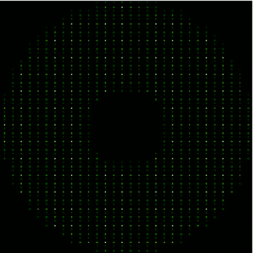
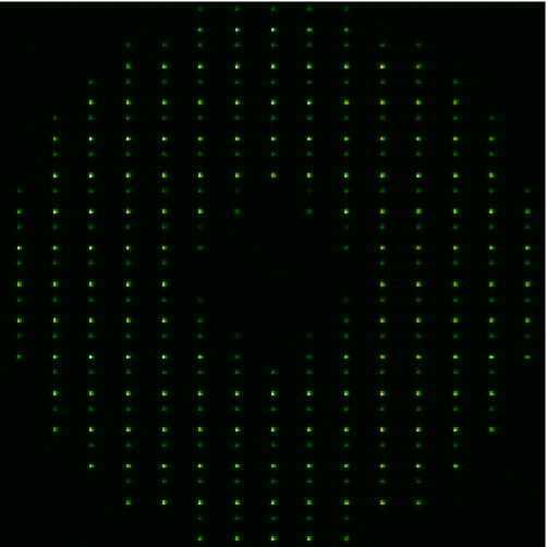
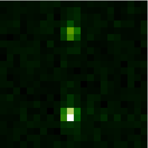
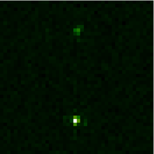
$30\times 30$ and $15\times 15$ SH images are computed after $100$ wave propagations through $32$ phase screens, representing the $32$ turbulent layers of the $C_{n}^{2}$ profile in Fig. 1. Then, $9$ cuts are performed on the electromagnetic field after each propagation, in order to get $900$ SH frames. These images are noise-free. Detection noises are added outside of the simulation code. Photon noise is modeled by a Poisson law and detector noise, assumed to be $\sigma_{e^{-}}=1~{}e^{-}$ per pixel and per frame, is modeled by a Gaussian law. Here, we assume that noise is statistically independent for different subapertures and stars. Typical SH frames and subaperture images are presented in Fig. 2.

Figure 2: Full SH images (averaged over 100 frames) and short-exposure subaperture images, obtained after propagation through turbulence and addition of detection noises. Left: $30\times 30$ geometry. Right: $15\times 15$ geometry.

4 Data processing

In this section we describe how we measure slopes and scintillation indexes from simulated SH images in Subsection 4.1, in order to make correlation maps. The bias subtraction process is detailed in Subsection 4.2.

4.1 Slopes and scintillation indexes extraction

Wavefront slopes and scintillation indexes for each star are calculated in each subaperture for all SH short-exposure images. Subapertures that are less than $95$ per cent illuminated are excluded from the analysis. To compute slopes $\mathbf{s_{m}}\left(\mathbf{\alpha}\right)$ in each of the two orthogonal “tip” and “tilt” directions, we use a centre of gravity (COG) algorithm. In order to separate the contributions of the two stars, and to limit the effects of noise, centroids are evaluated by delimiting windows around the stars. Boxes of $4\times 4$, $6\times 6$ and $8\times 8$ pixels are considered for the $30\times 30$ geometry, where the spots are not so much distorted because of turbulence ($\frac{d_{sub}}{r_{0}}\sim 1$). For the $15\times 15$ geometry, spots are more distorted. Indeed, the subaperture diameter is two times larger ($\frac{d_{sub}}{r_{0}}\sim 2$), and images are more affected by turbulence. So, we have to chose larger windows, and size of $8\times 8$, $10\times 10$, $12\times 12$, $14\times 14$ and $16\times 16$ pixels are considered. The positions of the boxes are determined by locating the mean position of the maximum of the spots in the subapertures. The total intensity corresponds to the total of all pixel intensities into the box. Scintillation index $\delta i_{m}\left(\mathbf{\alpha}\right)$ is derived by subtracting the mean intensity in the subaperture over the whole sequence of images $o_{m}\left(\mathbf{\alpha}\right)$, and by dividing the result by this same term. Slopes and scintillation indexes are extracted from noise-free and noisy images for comparison. Noise propagation occurred in the computation of slopes and scintillation indexes. As they are measured using a COG algorithm, noises contribution are then given by[9]:

$$\sigma_{\Delta\phi_{phot}}^{2}=\frac{\pi^{2}}{2}\frac{1}{N_{ph}}\left(\frac{N_{T}}{N_{D}}\right)^{2}$$ (8)

$$\sigma_{\Delta\phi_{det}}^{2}=\frac{\pi^{2}}{3}\left(\frac{\sigma_{e^{-}}}{N_{ph}}\right)^{2}\left(\frac{N_{s}^{2}}{N_{D}}\right)^{2}$$ (9)

for slope measurements. $N_{T}$ is the image full width at half maximum (FWHM), $N_{D}$ is the FWHM limited by diffraction and $N_{S}$ is the number of pixels for the COG calculation. However, in Eq. 8, $\sigma_{\Delta\phi_{phot}}^{2}$ does not depend on the size of the window. It has been shown that when $N_{S}\geq 2N_{D}$, $\sigma_{\Delta\phi_{phot}}^{2}$ can be written as[10]:

$$\sigma_{\Delta\phi_{phot}}^{2}=\frac{2}{N_{ph}}\left(\frac{N_{S}}{N_{D}}\right)$$ (10)

For scintillation measurements we have:

$$\sigma_{\delta i_{phot}}^{2}=\frac{1}{N_{ph}}$$ (11)

$$\sigma_{\delta i_{det}}^{2}=N_{S}^{2}\left(\frac{\sigma_{e^{-}}}{N_{ph}}\right)^{2}$$ (12)

For each kind of data, the total noise, $\sigma_{\Delta\phi_{noise}}^{2}$ for slopes and $\sigma_{\delta i_{noise}}^{2}$ for scintillation, is the sum of the terms $\sigma_{phot}^{2}$ and $\sigma_{det}^{2}$. The effects of the size of the window and the effects of noise on the $C_{n}^{2}$ measurement are investigated in Subsections 5.1 and 5.2.

4.2 Making of correlation maps and bias subtraction process

Auto-correlations (on a single star) and cross-correlations (between the two stars) are computed from slopes and scintillation indexes. In this simulated case, auto-correlations are evaluated for each star, and averaged, which increases the statistics by doubling the number of samples. Correlations are calculated for all separations between subapertures and represented as correlation maps. These maps show the mean correlation between all couples of subapertures having the same gap (Fig. 3), for the two kind of data, slopes and scintillation indexes. In the presence of measurement noises, these maps are biased.

Figure 3: Correlation maps for the $30\times 30$ geometry. The maps dimensions are 2 $\times$ number of subapertures-1, illustrating the correlation for all couples of subapertures. Top-left: slope auto-correlations in the x direction. Top-right: slope cross-correlations in the x direction. Bottom-left: scintillation auto-correlations. Top-right: scintillation cross-correlations.

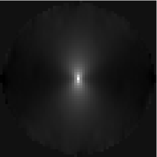
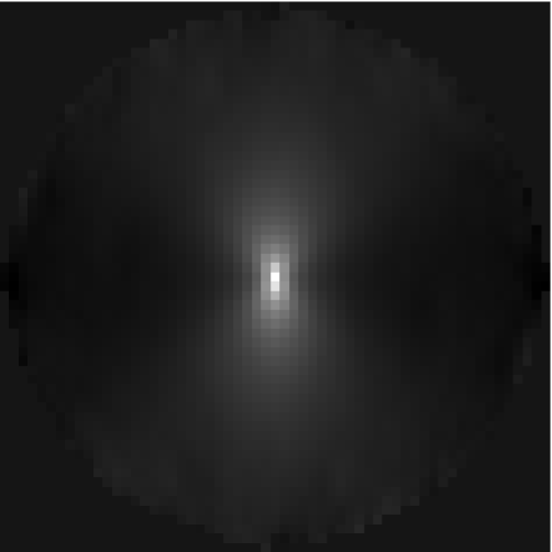
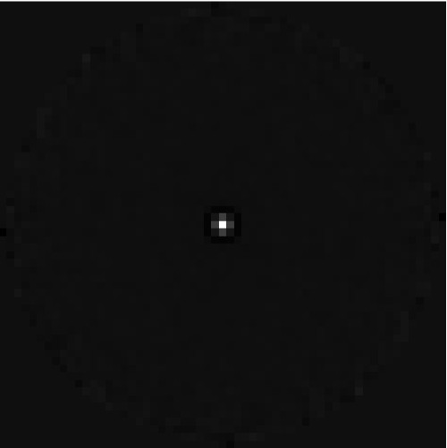
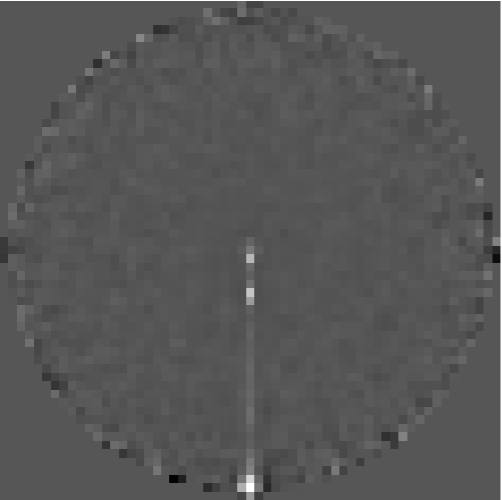
Assuming that the noise is statistically independent for different stars and subapertures, only the variance, namely the central value of the auto-correlation maps of slopes and scintillation are biased. A good way to estimate the bias is then to analytically calculate the noise using Eqs. 8, 9, 10, for slope auto-correlations and Eqs. 11, 12, for scintillation auto-correlations, knowing the number of photons $N_{ph}$ and the detector noise $\sigma_{e^{-}}$. As the two stars have different magnitudes, we apply different numbers of photons per subaperture and per frame in the formulae. The final bias is the mean of the biases given by each star. Once it is calculated, we just have to subtract it from the central value of the auto-correlation maps. The effect of the bias subtraction on the $C_{n}^{2}$ retrieval will be studied in Subsection 5.2.

5 $C_{n}^{2}$ restoration: results

The $C_{n}^{2}$ profiles reconstructed with the two SH geometries are presented and discussed in this section. We begin by studying the influence of the size of the window in Subsection 5.1. Then, the effects of measurement noises and bias subtraction are analyzed in Subsection 5.2. We finally compare the results with those obtained with other methods in Subsection 5.3, and the advantages of the two SH geometries are examined.

5.1 Influence of the COG window

As we said in Subsection 4.1, windows of different sizes are considered to compute slopes and intensities. Here, we only consider noise-free data. $C_{n}^{2}$ profiles reconstructed with the two geometries, for different sizes of window, are shown in Fig. 4. $C_{n}^{2}$ values lower than $1\times 10^{-19}~{}m^{-\frac{2}{3}}$ are automatically put to $1.3\times 10^{-19}~{}m^{-\frac{2}{3}}$ on the graph, for better understanding of the estimation. With the $30\times 30$ geometry we restore $32$ layers, that is to say the nominal number of layers of the input theoretical $C_{n}^{2}$ profile, while with the $15\times 15$ geometry, we only restore $20$ layers.

Figure 4: Impact of the size of the window for COG and intensity calculation on the reconstructed $C_{n}^{2}$ profile. Left: $30\times 30$ geometry. Right: $15\times 15$ geometry.

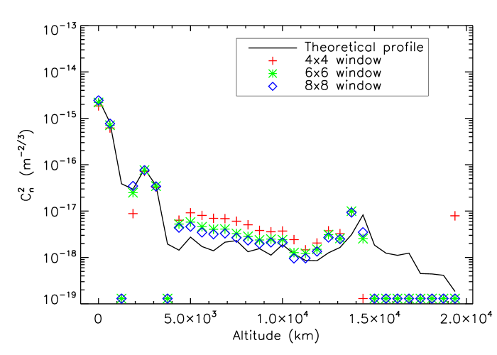
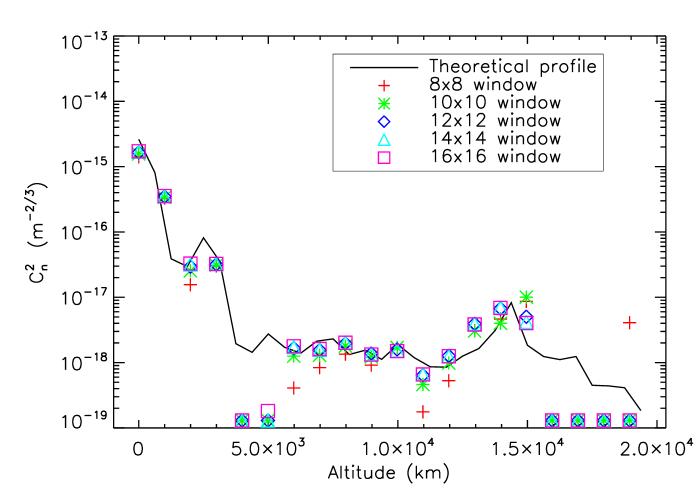
We can notice immediately that the size of the window introduces a slight bias in the $C_{n}^{2}$ profile measurement, and that for the two SH geometries. For the $30\times 30$ geometry, although the low altitude layers are almost well reconstructed with all sizes of window, the greatest differences occurred after $4~{}km$ of altitude. $C_{n}^{2}$ values are always over-estimated, but the smaller is the box, the higher is the over-estimation. The layer at $14~{}km$ is imperfectly reconstructed with the $6\times 6$ and $8\times 8$ windows, while it is not at all with the $4\times 4$ window. Layers after $15~{}km$ of altitude are not well estimated with the three sizes of window (cf. Subsection 5.3). For the $15\times 15$ geometry, we also observe that the reconstruction is improved when the size of the box increases. Identically, low altitude layers are almost well reconstructed. But, the plateau between $6~{}km$ and $12~{}km$ is better estimated when the box dimensions reach $10\times 10$ pixels. Results are quite similar for all sizes of window for layers between $12~{}km$ and $14~{}km$. The layer at $15~{}km$ is better evaluated when the box size reaches $12\times 12$ pixels. As for the other geometry, layers after $15~{}km$ of altitude are not well estimated with all sizes of window. Windows of $4\times 4$ and $6\times 6$ pixels were also tested, but results were too much biased so they are not presented.

This bias depending on the size of the window can be explained. When calculating slopes and intensities in little boxes, smaller than the whole subaperture, the spot is partially truncated. So, part of the flux is not taken into account for the COG calculation and the total intensity evaluation, leading to a biased estimation, that propagates in the $C_{n}^{2}$ profile retrieval. As a consequence, the size of the window must be chosen carefully. It must depend on the spot distortion and the signal to noise ratio (SNR) in the subaperture. The more the spot is distorted, the more the box has to be large, in order not to truncate too much the spot for the measurements. However, a larger window introduces more noise in the measurements (Eqs. 9, 10, 12). Moreover, if stars are too closed, the size of the box is implicitly limited. In the following, we keep windows of $8\times 8$ pixels for the $30\times 30$ geometry and windows of $12\times 12$ pixels for the $15\times 15$ geometry.

5.2 Influence of noise and effect of bias subtraction

Now we perform $C_{n}^{2}$ reconstruction from noisy data. The impact of noise propagation on the results is presented in Fig. 5.

Figure 5: Influence of noise on the $C_{n}^{2}$ profile reconstruction. Left: $30\times 30$ geometry. Right: $15\times 15$ geometry.

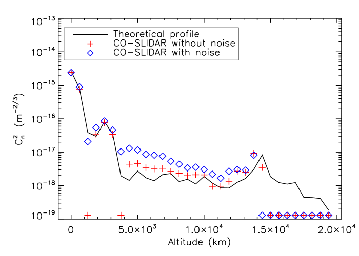
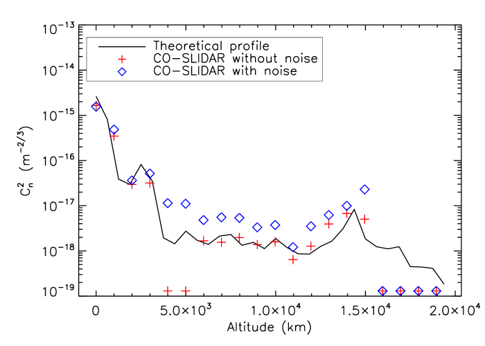
Noise adds an offset to all estimated $C_{n}^{2}$ values, with both geometries. Low altitude layers, until $4~{}km$ of altitude, are less impacted by this offset than layers between $4$ and $15~{}km$. Actually, these layers are mostly restored thanks to the scintillation signal. But, this signal has a poorer SNR than the slope signal. For the two geometries, the SNR on slopes and scintillation signals are detailed in Tables 1 and 2, using Eqs. 9, 10, 11, 12). These tables show that there is a good SNR on slope signal $\sigma_{\Delta\phi_{turb}}^{2}$, but it is very weak on the scintillation signal $\sigma_{\delta i_{turb}}^{2}$, even smaller than $1$ in the case of the $15\times 15$ geometry. This observation explains the bad estimation of the $C_{n}^{2}$ profile at altitudes between $4$ and $15~{}km$.

	SH $30\times 30$	SH $15\times 15$
$\sigma_{\Delta\phi_{turb}}^{2}$ ($rad^{2}$)	$3.4$	$9.5$
$\sigma_{\Delta\phi_{noise}}^{2}$ ($rad^{2}$)	$0.2$	$0.8$
$SNR$	$17$	$12$

Table 1: SNR on slope signal, for the two SH geometries.

	SH $30\times 30$	SH $15\times 15$
$\sigma_{\delta i_{turb}}^{2}$	$2.2\times 10^{-2}$	$8.3\times 10^{-3}$
$\sigma_{\delta i_{noise}}^{2}$	$8.7\times 10^{-3}$	$1.2\times 10^{-2}$
$SNR$	$2.7$	$0.7$

Table 2: SNR on scintillation signal, for the two SH geometries.

Then, we carry out the bias subtraction, as explained in Subsection 4.2, and using $\sigma_{\Delta\phi_{noise}}^{2}$ and $\sigma_{\delta i_{noise}}^{2}$ values presented in Table 1 and 2. They are subtracted from the central value of the auto-correlation maps. Bias-subtracted correlations are then used to restore the $C_{n}^{2}$ profile, and results are presented in Fig. 6.

Figure 6: Impact of bias-subtraction on the $C_{n}^{2}$ profile reconstruction. Left: $30\times 30$ geometry. Right: $15\times 15$ geometry.

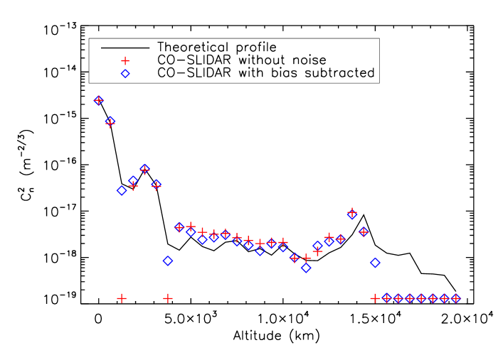
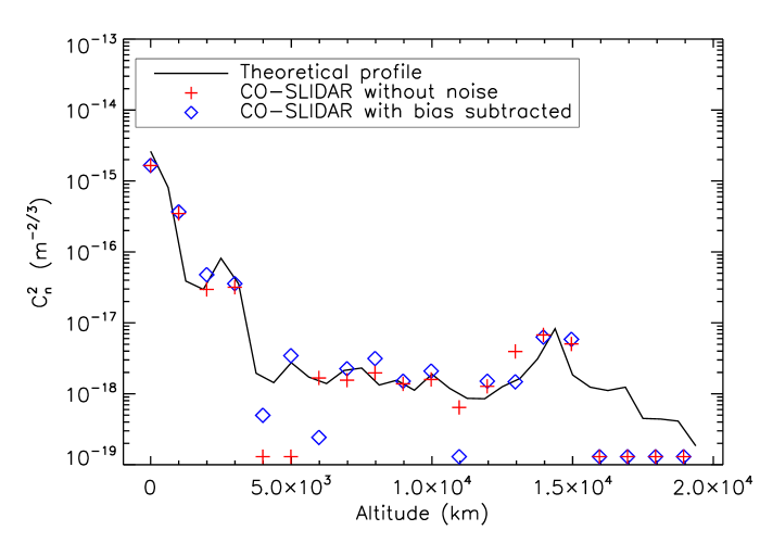
This correction nearly allows to restore the unbiased profile, especially with the $30\times 30$ geometry. Slight differences can be noticed with the $15\times 15$ geometry, probably due to the poor SNR, but the efficiency of the method is demonstrated.

5.3 Comparison with other methods, advantages of the two SH geometries

We finally compare $C_{n}^{2}$ profiles restored with CO-SLIDAR with $C_{n}^{2}$ profiles restored with slope data only or scintillation data only. Results are shown in Fig. 7.

Figure 7: Comparison of CO-SLIDAR with other methods. The bias has been subtracted in the three cases. Left: $30\times 30$ geometry. Right: $15\times 15$ geometry

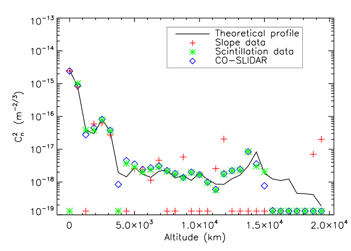
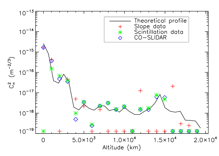
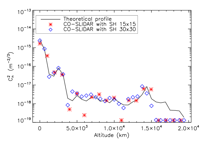
Comments are common to both geometries. In all cases, noisy data were used, and the bias has been calculated and subtracted. Slope data allow a good reconstruction of ground and low altitude layers, but they provide worse sensitivity at high altitude. Scintillation data perform a good reconstruction at low and high altitude, but do not permit to estimate the ground layer, as there is no scintillation on the pupil. This goes in the way of using both type of data to retrieve the $C_{n}^{2}$ profile. Actually, CO-SLIDAR combined the advantages of the two kind of data in a single instrument, and allows to estimate an accurate $C_{n}^{2}$ profile from the ground to $15~{}km$ of altitude, with these SH geometries. Layers after $15~{}km$ of altitude are not well reconstructed, neither with CO-SLIDAR nor slope nor scintillation data only. Indeed, after $15~{}km$, with these geometries, cross-correlations are blind to turbulence, according to Eq. 4. Information can then be provided by scintillation auto-correlations, but here the scintillation signal seems to be too weak to perform a good estimation of $C_{n}^{2}$ values. Better sensitivity could be achieved using smaller subapertures[11], but this would lead to deal with very low fluxes at subaperture level in an astronomical context. Anyway, these $C_{n}^{2}$ values are very small, $\leq 1\times 10^{-18}~{}m^{-\frac{2}{3}}$, and represent a negligible part of the whole turbulence. Nevertheless, these layers over $15~{}km$ of altitude could be estimated using a binary star with a smaller separation, to increase the altitude range sensitivity, but this would decrease the altitude resolution.

Finally, the performances of the two SH geometries need to be compared. Reconstructed profiles are presented in Fig. 8. We immediately notice the $30\times 30$ geometry has a better altitude resolution, about $500~{}m$, while the $15\times 15$ geometry only permits a resolution of about $1~{}km$, as forecast by Eq. 3. Both SH geometries allows a $C_{n}^{2}$ profile measurement from the ground to $15~{}km$ but do not permit to go over with reliable results, as explained before. The $15\times 15$ geometry, by collecting more flux, allows a better sky-coverage. Nevertheless, one has to be careful because if turbulence is too strong, images will be formed of speckles, leading to a difficult extraction of slopes and scintillation indexes. Both geometries have their advantages and they could be used together in order to cover a full observation night.

Figure 8: Comparison of the two SH geometries.

6 Conclusions and perspectives

In this paper, we detailed the performances of CO-SLIDAR in an end-to-end simulation, in a realistic astronomical case. Detection noises have been taken into account, and a way to subtract the bias from the measurements has been proposed and its efficiency demonstrated. CO-SLIDAR has been compared to other methods, highlighting the good complementarity of correlations of slopes and scintillation indexes, to provide turbulence sensitivity at low and high altitude. Two SH geometries have been proposed, each one with its proper advantages.

In order to perform complete on-sky validation, we acquired CO-SLIDAR data through an observation campaign on the MeO $1.5$-meter telescope, with the two SH geometries, at the Côte d’Azur Observatory, in South of France. Data processing is in progress, in order to estimate high-resolution $C_{n}^{2}$ profiles. SCO-SLIDAR, the extension of the method to a single source, should also be tested on single star data. Computation of error bars on the reconstructed profile has to be implemented, together with a refined study of the convergence noise. As sensitivity to the outer scale $L_{0}$ has been proved in a previous work[11], combined estimation of the two parameters is conceivable.

7 Acknowledgements

This work has been performed in the framework of a Ph.D Thesis supported by Onera, the French Aerospace Lab, and the French Direction Générale de l’Armement (DGA).

References

- [1] Fusco, T. and Costille, A., “Impact of Cn2 profile structure on wide-field AO performance,” in [SPIE Conference Series ], 7736 (2010).
- [2] Védrenne, N., Michau, V., Robert, C., and Conan, J., “Cn2 profile measurement from shack-hartmann data,” Opt. Lett. 32(18), 2659–2661 (2007).
- [3] Wilson, R. W., “SLODAR: measuring optical turbulence altitude with a Shack-Hartmann wavefront sensor,” Mon. Not. R. Astron. Soc. 337, 103–108 (2002).
- [4] Fuchs, A., Tallon, M., and Vernin, J., “Focusing on a Turbulent Layer: Principle of the “Generalized SCIDAR”,” Publ. Astron. Soc. Pac. 110, 86–91 (1998).
- [5] Kornilov, V., Tokovinin, A. A., Vozyakova, O., Zaitsev, A., Shatsky, N., Potanin, S. F., and Sarazin, M. S., “MASS: a monitor of the vertical turbulence distribution,” in [SPIE Conference Series ], 4839, 837–845 (2003).
- [6] Robert, C., Voyez, J., Védrenne, N., and Mugnier, L., “Cn2 profile from Shack-Hartmann data with CO-SLIDAR data processing,” ArXiv e-prints (2011).
- [7] Védrenne, N., Bonnefois Montmerle, A., Robert, C., Michau, V., Montri, J., and Fleury, B., “Cn2 profile measurement from Shack-Hartmann data: experimental validation and exploitation,” in [SPIE Conference Series ], 7828 (2010).
- [8] Robert, C., Conan, J., Michau, V., Fusco, T., and Védrenne, N., “Scintillation and phase anisoplanatism in Shack-Hartmann wavefront sensing,” J. Opt. Soc. Am. A 23, 613–624 (2006).
- [9] Rousset, G., Primot, J., and Fontanella, J. C., “Visible wavefront sensor development.,” LEST Foundation, Technical Report, No. 28, p. 17 - 33 28, 17–33 (1987).
- [10] Thomas, S., Fusco, T., Tokovinin, A., Nicolle, M., Michau, V., and Rousset, G., “Comparison of centroid computation algorithms in a Shack-Hartmann sensor,” Mon. Not. R. Astron. Soc. 371, 323–336 (Sept. 2006).
- [11] Voyez, J., Robert, C., Fleury, B., Védrenne, N., Michau, V., Fusco, T., and Samain, E., “Cn2 profilometry from Shack-Hartmann data: model and experiment,” in [Adaptive Optics for Extremely Large Telescopes II ], (to be published).