Low rank approximation for the numerical simulation of high dimensional Lindblad and Riccati equations

Abstract

A systematic numerical approach to approximate high dimensional Lindblad equations is described. It is based on a deterministic rank $m$ approximation of the density operator, the rank $m$ being the only parameter to adjust. From a known initial value, this rank $m$ approximation gives at each time-step an estimate of the largest $m$ eigen-values with their eigen-vectors of the density operator. A numerical scheme is proposed. Its numerical efficiency in the case of a rank $m=12$ approximation is demonstrated for oscillation revivals of $50$ atoms interacting resonantly with a slightly damped coherent quantized field of $200$ photons. The approach may be employed for other similar equations. We in particularly show how to adapt such low-rank approximation for Riccati differential equations appearing in Kalman filtering.

1 Introduction

Numerical simulations of high dimensional Lindblad equations are routinely performed using ensemble averages of quantum Monte-Carlo trajectories [2, 9, 5]. We propose here another approach that can be also adapted to high dimensional matrix Riccati equations. This approach consists in approximating the evolution of the $n\times n$ density matrix $\rho$ solution to the differential Lindblad equation using a reduced dynamics on the set of density matrices of some fixed rank $m<n$. This reduced dynamics is obtained by taking the orthogonal projection of $\frac{d}{dt}\rho$ onto the tangent space to this set of matrices of rank $m$.

Such an approximation strategy, based on orthogonal projections onto low dimensional manifolds, has already been proposed in [4, 7] in the context of quantum filtering. The goal then was to construct a reduced order quantum filter for a spin-spring system. The submanifold on which the dynamics was projected was the (real) 4-dimensional manifold constructed with the tensor products of arbitrary two-level states and pure coherent states. In [1], a geometric approach to study the stability of low-rank solutions for matrix Riccati differential equations has been likewise developed. We combine here the ideas of [4] and [1]. We focus on the Lindblad case. The Riccati case is addressed in appendix A without numerical simulations. Nevertheless, in both cases, the proposed approximation depends only on one adjustable parameter, the low-order rank $m$.

When the size $n\times n$ of the density matrix exceeds the computing possibilities available –which is often the case in practice even for rather simple physically relevant systems–, such an approximation can be very useful to compute the (approximate) time evolution of $\rho$ from a known initial value with rank smaller than or equal to $m$. This approximation strategy is tested here on oscillation revivals of $N_{a}$ atoms in a slightly damped mesoscopic field with $\bar{n}$ photons in average [8]. In a first stage, we consider the original half-spin/spring case [3] with $N_{a}=1$ and $\bar{n}=15$. For a photon lifetime in the order of one hundred vacuum Rabi periods, we compare the numerical solution $\rho(t)$ to the Lindblad equation (computed for reference) with different numerical low-rank solutions from $m=2$ to $6$. Our results show a very satisfactory agreement. We next take the much larger values $N_{a}=50$ and $\bar{n}=200$. The density matrix is then too large for an explicit comparison with the direct numerical integration of the Lindblad differential equation to be possible using a standard computer ($n\sim 15000$). For a photon lifetime in the order of ten thousands vacuum Rabi periods, we have checked that our numerical solution using a reduced model of rank $m=12$ is consistent with the analytic damping model proposed in [8]. We also observe numerically that the larger the rank $m$, the more accurate the approximation.

Our article is articulated as follows. We derive in Section 2 the low rank dynamics approximating the Lindblad equation. We describe the numerical scheme we use in Section 3. In both sections, our general purpose strategy is specifically adjusted to account for the fact that, usually, the Hamiltonian part dominates the decoherence part. Section 4 presents our numerical experiments on oscillation revivals. We draw some conclusions in Section 5. In appendix A, a similar low-rank approximated dynamics is derived for the matrix Riccati equation appearing in Kalman filtering. Such low-rank approximates of the covariance matrix could be eventually useful in data assimilation for large scale systems as those governed by partial differential equations.

Acknowledgements

The authors thank Silvère Bonnabel, Michel Brune, Michel Devoret, Jean-Michel Raimond for useful references and stimulating interactions. The authors were partially supported by the ANR, Projet Blanc EMAQS ANR-2011-BS01-017-01.

2 The Low rank differential equations

Consider a Lindblad equation with, for simplicity (see last paragraph of this section), a single decoherence operator $L$,

$$\frac{d}{dt}\rho=-i[H,\rho]-\tfrac{1}{2}(L^{\dagger}L\rho+\rho L^{\dagger}L)+L\rho L^{\dagger},$$ (1)

where $\rho$ is $n\times n$ non-negative Hermitian matrix with $\text{Tr}\left(\rho\right)=1$, $H$ is a $n\times n$ Hermitian matrix and $L$ is a $n\times n$ matrix. Our purpose is to approximate, for $n$ large, the above dynamics on the set of non-negative Hermitian matrices of rank $m$, $m$ being an integer presumably much smaller than $n$, prescribed beforehand. We now formalize this.

A density $\rho$ of rank $m<n$ can be decomposed as

$$\rho=U\sigma U^{\dagger}$$ (2)

where $\sigma$ is a $m\times m$ strictly positive Hermitian matrix, $U$ a $n\times m$ matrix with $U^{\dagger}U={\mathbb{I}}_{m}$, and ${\mathbb{I}}_{m}$ of course denotes the $m\times m$ identity matrix. The set of non-negative Hermitian matrices of rank $m$ and trace one can be seen as a sub-manifold, denoted by ${\mathcal{D}}_{m}$, of the Euclidean space of $n\times n$ Hermitian matrices equipped with the Frobenius scalar product. For $\rho\in{\mathcal{D}}_{m}$, $\frac{d}{dt}\rho$ given by (1) does not belong in general to the tangent space to ${\mathcal{D}}_{m}$ at $\rho$. The rank is therefore not necessarily preserved by the evolution governed by (1). To correct for this, the most natural option is to consider, for any $\rho\in{\mathcal{D}}_{m}$, the orthogonal projection of $\frac{d}{dt}\rho$ given by (1) onto the tangent space to ${\mathcal{D}}_{m}$ at $\rho$. Denoting by $\Pi_{m}^{\rho}$ the projection operator, we therefore consider the differential equation

$$\frac{d}{dt}\rho=\Pi_{m}^{\rho}\left(-i[H,\rho]-\tfrac{1}{2}(L^{\dagger}L\rho+\rho L^{\dagger}L)+L\rho L^{\dagger}\right)$$ (3)

set on ${\mathcal{D}}_{m}$, which can be seen as a rank $m$ approximation of (1).

Making the approach practical requires to now give an explicit formulation of such a rank $m$ approximation. A lifting procedure, inspired from [1] and described in some more details below, consists in introducing two coupled differential equations for $U$ and $\sigma$ corresponding to the generic decomposition (2) for $\rho\in{\mathcal{D}}_{m}$:

$$\frac{d}{dt}U =-iAU+({\mathbb{I}}_{n}-UU^{\dagger})\left(-i(H-A)-\tfrac{1}{2}L^{\dagger}L+LU\sigma U^{\dagger}L^{\dagger}U\sigma^{-1}U^{\dagger}\right)U,$$ (4)

$$\frac{d}{dt}\sigma =-i[U^{\dagger}(H-A)U,\sigma]-\tfrac{1}{2}(U^{\dagger}L^{\dagger}LU\sigma+\sigma U^{\dagger}L^{\dagger}LU)+U^{\dagger}LU\sigma U^{\dagger}L^{\dagger}U$$

$$\qquad+\tfrac{1}{m}\text{Tr}\left((L^{\dagger}({\mathbb{I}}_{n}-UU^{\dagger})L\leavevmode\nobreak\ U\sigma U^{\dagger}\right){\mathbb{I}}_{m}.$$ (5)

In (4)-(5), $A$ denotes an arbitrary Hermitian operator that may depend on time. Then standard manipulations, which we omit here for brevity, show that

• $U^{\dagger}U$ remains equal to ${\mathbb{I}}_{m}$,

• $\sigma$ remains Hermitian, positive and of trace one,

and that the evolution of $\rho=U\sigma U^{\dagger}$ then solves (3), which in this particular instance reads

$$\frac{d}{dt}\rho=-i[H,\rho]-\tfrac{1}{2}(L^{\dagger}L\rho+\rho L^{\dagger}L)+L\rho L^{\dagger}-({\mathbb{I}}_{n}-P_{\rho})L\rho L^{\dagger}({\mathbb{I}}_{n}-P_{\rho})\\ +\tfrac{\text{Tr}\left(L\rho L^{\dagger}({\mathbb{I}}_{n}-P_{\rho})\right)}{m}P_{\rho},$$ (6)

where $P_{\rho}=UU^{\dagger}$ only depends on $\rho$ since it corresponds to the orthogonal projection on the image of $\rho$.

Notice that (6) does not depend on the arbitrary matrix $A$: its entries can be seen as gauge degrees of freedom. The specific choice $A=H$ yields

$$\frac{d}{dt}U =-iHU+({\mathbb{I}}_{n}-UU^{\dagger})\left(-\tfrac{1}{2}L^{\dagger}L+LU\sigma U^{\dagger}L^{\dagger}U\sigma^{-1}U^{\dagger}\right)U,$$ (7)

$$\frac{d}{dt}\sigma =-\tfrac{1}{2}(U^{\dagger}L^{\dagger}LU\sigma+\sigma U^{\dagger}L^{\dagger}LU)+U^{\dagger}LU\sigma U^{\dagger}L^{\dagger}U$$

$$\qquad+\tfrac{1}{m}\text{Tr}\left((L^{\dagger}({\mathbb{I}}_{n}-UU^{\dagger})L\leavevmode\nobreak\ U\sigma U^{\dagger}\right){\mathbb{I}}_{m},$$ (8)

where we note that $H$ only appears in the dynamics for $U$ and not in the dynamics of $\sigma$, a choice that is particularly appropriate when $H$ dominates $L$. In that case indeed, (8) may be understood as a slow evolution as compared to the dynamics (7). The efficiency of our numerical procedure, described in the next section, will significantly benefit from this particular decomposition.

We now explain how we obtain (4) and (5). A $n\times n$ Hermitian matrix $\xi$ in the tangent space at $\rho=U\sigma U^{\dagger}$ to ${\mathcal{D}}_{m}$ admits the parameterization

$$\xi=i[\eta,\rho]+U\varsigma U^{\dagger}=U\big{(}i[U^{\dagger}\eta U,\sigma]+\varsigma\big{)}U^{\dagger}$$ (9)

where $\eta$ is any $n\times n$ Hermitian matrix and $\varsigma$ any $m\times m$ Hermitian matrix with zero trace. This results from the definition of the tangent map of the submersion $(U,\sigma)\mapsto U\sigma U^{\dagger}$ with the infinitesimal variations $\delta U=\imath\eta U$ and $\delta\sigma=\varsigma$. The parameterization (9) is onto, but not one-to-one: note that different $\eta$ and $\varsigma$ may indeed yield the same $\xi$. The projection $\Pi_{m}^{\rho}(\frac{d}{dt}\rho)$ corresponds to the tangent vector $\xi$ associated to $\eta$ and $\varsigma$ minimizing

$$\text{Tr}\left(\Big{(}S\rho+\rho S^{\dagger}+L\rho L^{\dagger}-i[\eta,\rho]-U\varsigma U^{\dagger}\Big{)}^{2}\right),$$

where $S=-iH-L^{\dagger}L/2$. The first order stationary conditions versus $\varsigma$ and $\eta$ read

$$U^{\dagger}\big{(}S\rho+\rho S^{\dagger}+L\rho L^{\dagger}-i[\eta,\rho]-U\varsigma U^{\dagger}\big{)}U =\lambda{\mathbb{I}}_{m}\quad,$$

$$\big{[}S\rho+\rho S^{\dagger}+L\rho L^{\dagger}-i[\eta,\rho]-U\varsigma U^{\dagger},\rho\big{]}=0,$$

where the real scalar $\lambda$ is implicitly given by the constraint $\text{Tr}\left(\varsigma\right)=0$. The first equation yields

$$\varsigma=U^{\dagger}\big{(}S\rho+\rho S^{\dagger}+L\rho L^{\dagger}-i[\eta,\rho]\big{)}U-\tfrac{1}{m}\text{Tr}\left(U^{\dagger}(S\rho+\rho S^{\dagger}+L\rho L^{\dagger})U\right){\mathbb{I}}_{m}.$$ (10)

We insert this value of $\varsigma$ into the second equation and obtain, after some easy manipulations using $U^{\dagger}U={\mathbb{I}}_{m}$,

$$({\mathbb{I}}_{n}-P)\big{(}S\rho+L\rho L^{\dagger}-i\eta\rho\big{)}\rho=\rho\big{(}\rho S^{\dagger}+L\rho L^{\dagger}+i\rho\eta\big{)}({\mathbb{I}}_{n}-P)$$

where $P=UU^{\dagger}$ is the orthogonal projector on the image of $U$. This matrix equation admits the following general solution

$$\eta=-i({\mathbb{I}}_{n}-P)\big{(}SP+L\rho L^{\dagger}U\sigma^{-1}U^{\dagger}\big{)}+i\big{(}PS^{\dagger}+U\sigma^{-1}U^{\dagger}L\rho L^{\dagger}\big{)}({\mathbb{I}}_{n}-P)\\ -PAP-({\mathbb{I}}_{n}-P)A({\mathbb{I}}_{n}-P)$$ (11)

where $A$ is an arbitrary Hermitian operator. Then, using $U^{\dagger}P=U^{\dagger}$ and $PU=U$, $\varsigma$ given by (10) reads

$$\varsigma=-i[U^{\dagger}HU,\sigma]-\tfrac{1}{2}(U^{\dagger}L^{\dagger}LU\sigma+\sigma U^{\dagger}L^{\dagger}LU)+U^{\dagger}LU\sigma U^{\dagger}L^{\dagger}U\\ +\tfrac{1}{m}\text{Tr}\left((L^{\dagger}({\mathbb{I}}_{n}-UU^{\dagger})L\leavevmode\nobreak\ U\sigma U^{\dagger}\right){\mathbb{I}}_{m}+i[U^{\dagger}AU,\sigma]$$ (12)

The derivatives $\frac{d}{dt}U=\imath\eta U$ and $\frac{d}{dt}\sigma=\varsigma$ respectively give (4) and (5).

We finally note that, for clarity, we have deliberately restricted our exposition to the case of a single decoherence term in (1). The generalization to an arbitrary number of decoherence terms

$$\frac{d}{dt}\rho=-i[H,\rho]+\sum_{\nu}L_{\nu}\rho L_{\nu}^{\dagger}-\tfrac{1}{2}(L_{\nu}^{\dagger}L_{\nu}\rho+\rho L_{\nu}^{\dagger}L_{\nu}),$$

is straightforward: (7) and (8) become

$$\frac{d}{dt}U =-iHU+({\mathbb{I}}_{n}-UU^{\dagger})\left(\sum_{\nu}-\tfrac{1}{2}L_{\nu}^{\dagger}L_{\nu}+L_{\nu}U\sigma U^{\dagger}L_{\nu}^{\dagger}U\sigma^{-1}U^{\dagger}\right)U$$

$$\frac{d}{dt}\sigma =\sum_{\nu}\tfrac{-1}{2}(U^{\dagger}L_{\nu}^{\dagger}L_{\nu}U\sigma+\sigma U^{\dagger}L_{\nu}^{\dagger}L_{\nu}U)+U^{\dagger}L_{\nu}U\sigma U^{\dagger}L_{\nu}^{\dagger}U$$

$$\qquad+\tfrac{1}{m}\text{Tr}\left(\sum_{\nu}(L_{\nu}^{\dagger}({\mathbb{I}}_{n}-UU^{\dagger})L_{\nu}\leavevmode\nobreak\ U\sigma U^{\dagger}\right){\mathbb{I}}_{m}.$$

3 Numerical integrator

For a positive integer $k$ and the timestep $\delta t$, we denote by $U_{k}$ and $\sigma_{k}$ the numerical approximations of $U(k\delta t)$ and $\sigma(k\delta t)$ solutions to (7) and (8) respectively. The evolution from time $k\delta t$ to time $(k+1)\delta t$ is split into the following three steps:

• The first step consists in an approximation of the free Hamiltonian evolution $U_{{k\!+\!\text{\tiny$\tfrac{1}{3}$}}}=e^{-(i\delta t/2)H}U_{k}$. For the simulations of Section 4, we choose a (formal) third-order expansion:

  $$U_{{k\!+\!\text{\tiny$\tfrac{1}{3}$}}}=\left({\mathbb{I}}_{n}-\tfrac{i\delta t}{2}H-\tfrac{\delta t^{2}}{8}H^{2}+i\tfrac{\delta t^{3}}{48}H^{3}\right)U_{k}.$$ (13)

  We however note that, of course, other choices are possible. In particular, time integrators more adapted to the time discretization of the Schrödinger may be employed (see [6] and references therein). We will not proceed in this direction in the present work and, should need be, hope to return to this issue in future works.

• The second step consists in updating both $U$ and $\sigma$ now accounting for $L$; we set

  $$U_{{k\!+\!\text{\tiny$\tfrac{2}{3}$}}}=U_{{k\!+\!\text{\tiny$\tfrac{1}{3}$}}}+\delta t({\mathbb{I}}_{n}-U_{{k\!+\!\text{\tiny$\tfrac{1}{3}$}}}U_{{k\!+\!\text{\tiny$\tfrac{1}{3}$}}}^{\dagger})\left(-\tfrac{1}{2}L^{\dagger}LU_{{k\!+\!\text{\tiny$\tfrac{1}{3}$}}}+LU_{{k\!+\!\text{\tiny$\tfrac{1}{3}$}}}\sigma_{k}U_{{k\!+\!\text{\tiny$\tfrac{1}{3}$}}}^{\dagger}L^{\dagger}U_{{k\!+\!\text{\tiny$\tfrac{1}{3}$}}}\sigma_{k}^{-1}\right)$$ (14)

  and, in two stages,

  $$\sigma_{{k\!+\!\text{\tiny$\tfrac{1}{2}$}}} = \sigma_{k}+\delta t\leavevmode\nobreak\ U_{{k\!+\!\text{\tiny$\tfrac{1}{3}$}}}^{\dagger}LU_{{k\!+\!\text{\tiny$\tfrac{1}{3}$}}}\sigma_{k}U_{{k\!+\!\text{\tiny$\tfrac{1}{3}$}}}^{\dagger}L^{\dagger}U_{{k\!+\!\text{\tiny$\tfrac{1}{3}$}}}$$ (15)

  $$+\delta t\leavevmode\nobreak\ \frac{\text{Tr}\left((U_{{k\!+\!\text{\tiny$\tfrac{1}{3}$}}}^{\dagger}L^{\dagger}LU_{{k\!+\!\text{\tiny$\tfrac{1}{3}$}}}-U_{{k\!+\!\text{\tiny$\tfrac{1}{3}$}}}^{\dagger}L^{\dagger}U_{{k\!+\!\text{\tiny$\tfrac{1}{3}$}}}U_{{k\!+\!\text{\tiny$\tfrac{1}{3}$}}}^{\dagger}LU_{{k\!+\!\text{\tiny$\tfrac{1}{3}$}}})\sigma_{k}\right)\leavevmode\nobreak\ {\mathbb{I}}_{m}}{m},$$

  followed by

  $$\sigma_{k+1}=\frac{({\mathbb{I}}_{m}-\tfrac{\delta t}{2}U_{{k\!+\!\text{\tiny$\tfrac{1}{3}$}}}^{\dagger}L^{\dagger}LU_{{k\!+\!\text{\tiny$\tfrac{1}{3}$}}})\sigma_{k\!+\!\text{\tiny$\tfrac{1}{2}$}}({\mathbb{I}}_{m}-\tfrac{\delta t}{2}U_{{k\!+\!\text{\tiny$\tfrac{1}{3}$}}}^{\dagger}L^{\dagger}LU_{{k\!+\!\text{\tiny$\tfrac{1}{3}$}}})}{\text{Tr}\left(({\mathbb{I}}_{m}-\tfrac{\delta t}{2}U_{{k\!+\!\text{\tiny$\tfrac{1}{3}$}}}^{\dagger}L^{\dagger}LU_{{k\!+\!\text{\tiny$\tfrac{1}{3}$}}})\sigma_{k\!+\!\text{\tiny$\tfrac{1}{2}$}}({\mathbb{I}}_{m}-\tfrac{\delta t}{2}U_{{k\!+\!\text{\tiny$\tfrac{1}{3}$}}}^{\dagger}L^{\dagger}LU_{{k\!+\!\text{\tiny$\tfrac{1}{3}$}}})\right)}.$$ (16)

  We note that this two-stage update corresponds to a slight modification of the explicit Euler scheme so that it preserves both positiveness and the trace. In particular, the motivation for using (16) can be understood from the following considerations (which can be adapted to many similar contexts). Momentarily omitting its rightmost term for simplicity, we observe that, with obvious notation, (8) is of the form $\displaystyle\frac{d}{dt}\sigma=W\,\sigma+\sigma\,W^{\dagger}+Z\,\sigma\,Z^{\dagger}$. Introducing the auxiliary variables $\tilde{\sigma}=B\,\sigma\,B^{\dagger}$ and $\tilde{Z}=B\,Z\,B^{-1}$ with $B$ solution to $\displaystyle\frac{d}{dt}B=-BW$, we see that $\displaystyle\frac{d}{dt}\tilde{\sigma}=\tilde{Z}\,\tilde{\sigma}\,\tilde{Z}^{\dagger}$, an equation that can be simply integrated using the first order forward Euler scheme $\tilde{\sigma}_{k+1}=\tilde{\sigma}_{k+1/2}+\delta t/2\,\,\tilde{Z}_{k+1/2}\,\tilde{\sigma}_{k+1/2}\,\tilde{Z}_{k+1/2}^{\dagger}$. Expressed in the original unknown $\sigma$, this scheme gives the numerator of (16) up to $\delta t^{2}$ terms and automatically preserves positiveness. The preservation of the trace is then ensured by the normalization in (16).

• The third step is similar to the first step, the third-order approximation of $U_{k+1}=e^{-(i\delta t/2)H}U_{{k\!+\!\text{\tiny$\tfrac{2}{3}$}}}$, this time followed by an orthonormalization (a procedure formally denoted by $\Upsilon$) to ensure $U_{k+1}^{\dagger}U_{k+1}={\mathbb{I}}_{m}$:

  $$U_{k+1}=\Upsilon\Big{(}\left({\mathbb{I}}_{n}-\tfrac{i\delta t}{2}H-\tfrac{\delta t^{2}}{8}H^{2}+i\tfrac{\delta t^{3}}{48}H^{3}\right)U_{{k\!+\!\text{\tiny$\tfrac{2}{3}$}}}\Big{)}.$$ (17)

Three comments, different in nature, are in order.

Computational cost

The above numerical scheme essentially uses right multiplications of $H$, $L$, $L^{\dagger}$ by $n\times m$ matrices, as, for example, the products $HU$, $H^{2}U=H(HU)$, $LU$, $L^{\dagger}(LU)$. To evaluate such products does not require string $n\times n$ matrices since usually $H$ and $L$ are defined as tensor products of operators of small dimensions. When $n$ is very large and $m$ is small, this point is crucial for an efficient numerical implementation of the approach. In particular evaluations of products like $HU$ or $LU$ can be easily parallelized.

Formal error estimator

To obtain an empirical estimate of the error committed when using the low rank approximation, we may follow [4] and compute the Frobenius norm of $\dot{\rho}=\frac{d}{dt}\rho$ and $\dot{\rho}_{\perp}=\dot{\rho}-\Pi_{m}^{\rho}(\dot{\rho})$ at each time step. If the Frobenius norm of $\dot{\rho}_{\perp}$ is much smaller than that of $\dot{\rho}$, then the approximation is considered valid. From (6), we have the following general formulae for any $\rho\in{\mathcal{D}}_{m}$, any Hermitian operator $H$ and any not necessarily Hermitian operator $L$:

$$\Pi_{m}^{\rho}\Big{(}[H,\rho]\Big{)} =[H,\rho]$$

$$\Pi_{m}^{\rho}\Big{(}-\tfrac{1}{2}(L^{\dagger}L\rho+\rho L^{\dagger}L)+L\rho L^{\dagger}\Big{)} =-\tfrac{1}{2}(L^{\dagger}L\rho+\rho L^{\dagger}L)+L\rho L^{\dagger}$$

$$\qquad-({\mathbb{I}}_{n}-P_{\rho})L\rho L^{\dagger}({\mathbb{I}}_{n}-P_{\rho})+\tfrac{\text{Tr}\left(L\rho L^{\dagger}({\mathbb{I}}_{n}-P_{\rho})\right)}{m}P_{\rho}.$$

Thus we have,

$$\dot{\rho}_{\perp}=({\mathbb{I}}_{n}-P_{\rho})L\rho L^{\dagger}({\mathbb{I}}_{n}-P_{\rho})-\tfrac{\text{Tr}\left(L\rho L^{\dagger}({\mathbb{I}}_{n}-P_{\rho})\right)}{m}P_{\rho}$$ (18)

where $P_{\rho}=UU^{\dagger}$ since $\rho=U\sigma U^{\dagger}$. Classical computations using standard properties of the trace show that, at each time step, $\text{Tr}\left(\dot{\rho}^{2}\right)$ and $\text{Tr}\left(\dot{\rho}_{\perp}^{2}\right)$ may be numerically evaluated with a complexity similar to the complexity of the numerical scheme. There is no need to explicitly compute $\dot{\rho}$ and $\dot{\rho}_{\perp}$ as $n\times n$ matrices before taking their Frobenius norm.

Choice of the initial condition

Initial conditions for $\sigma$ and $U$ need to be deduced from a given initial condition $\rho_{0}$. When the rank of $\rho_{0}$ is larger than or equal to $m$, we form $\sigma_{0}$ as the diagonal matrix consisting of the largest $m$ eigenvalues of $\rho_{0}$ with sum normalized to one and we form $U_{0}$ using the associated eigenvectors. When the rank of $\rho_{0}$ is strictly less than $m$ then we proceed as follows.

Assume in a first step that $\rho_{0}$ is a pure state $|\psi_{0}\rangle\langle\psi_{0}|$. It is then natural to take for $\sigma_{0}$ a diagonal matrix where the first diagonal element is $1-(m-1)\epsilon$ and the over ones are equal to $\epsilon$. Here $\epsilon$ is a positive number much smaller than $1$ (typically $10^{-5}$). Then $U_{0}$ is constructed, up to an orthonormalization preserving the first column, with $|\psi_{0}\rangle$ as the first column, $H|\psi_{0}\rangle$ as the second column, …, $H^{m-1}|\psi_{0}\rangle$ as the last column.

When the rank of $\rho_{0}$ is strictly larger than $1$ (but still strictly less than $m$), one can easily imagine the following mixed procedure: put the non-zero eigenvalues in the first diagonal elements of $\sigma_{0}$, their associated eigenvectors in the first columns of $U_{0}$, set the remaining diagonal elements of $\sigma_{0}$ to $\epsilon$ and complete the remaining columns of $U_{0}$ by iterates of $H$ on these eigenvectors.

4 Numerical tests for oscillation revivals

The collective behavior of $N_{a}$ atoms resonantly interacting with a quantized single-mode field trapped in an almost perfect cavity is modeled by the following Lindblad master equation (see, e.g., [8])

$$\frac{d}{dt}\rho=\frac{\Omega_{0}}{2}[\text{\bf{a}}^{\dagger}J^{-}-\text{\bf{a}}J^{+},\rho]-\kappa(\text{\bf{n}}\rho/2+\rho\text{\bf{n}}/2-\text{\bf{a}}\rho\text{\bf{a}}^{\dagger})$$ (19)

where $\Omega_{0}>0$ is the coupling strength (vacuum Rabi pulsation), a the field annihilation operator, $\text{\bf{n}}=\text{\bf{a}}^{\dagger}\text{\bf{a}}$ the field photon-number operator and $\kappa>0$ the inverse of the single photon life-time. The $N_{a}$ atoms are described here with the spin $J=N_{a}/2$ representation. It involves the $N_{a}+1$ Dicke states $|J,-N_{a}/2\rangle$, $|J,(-N_{a}+1)/2\rangle$, …, $|J,N_{a}/2\rangle$. These Dicke states are labelled by the index $\mu=0$ to $\mu=N_{a}$ and are denoted by $|\mu\rangle$: for $\mu=0$ all atoms are in the same ground state; for $\mu=N_{a}+1$ all atoms are in the same excited state. With this notation, the atomic lowering operator, $J^{-}=(J^{+})^{\dagger}$, is given by $J^{-}|\mu\rangle=\sqrt{\mu(N_{a}-\mu)}|\mu-1\rangle$, $\mu=0,\ldots,N_{a}$.

For $N_{a}=1$ atom initially in the excited state, a field initially in a coherent state with $\bar{n}=15$ photons (truncation to $30$ photons), and a damping factor $\kappa=\Omega_{0}/500$, we have compared, until the first revival appearing around $t=\frac{2\pi}{\Omega_{0}/2\sqrt{\bar{n}}}$, low-rank trajectories, solutions to (7,8), with the original full-rank trajectory solution to (1) where $H=i\frac{\Omega_{0}}{2}(\text{\bf{a}}^{\dagger}J^{-}-\text{\bf{a}}J^{+})$ and $L=\sqrt{\kappa}\text{\bf{a}}$. In this simple case performing the full-rank simulation for the sake of comparison is indeed feasible. Initializations of $U$ and $\sigma$ are performed according to the procedure explained at the end of Section 3.

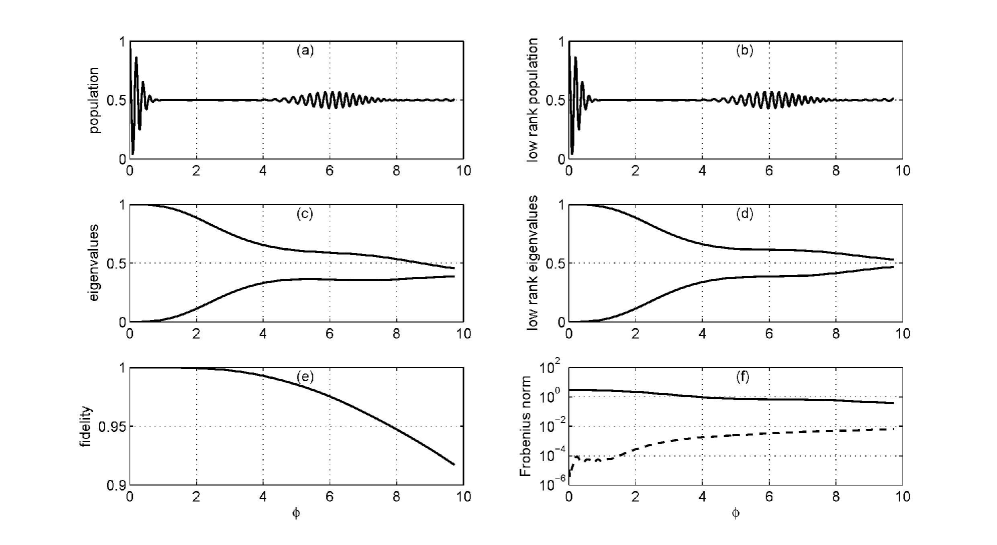
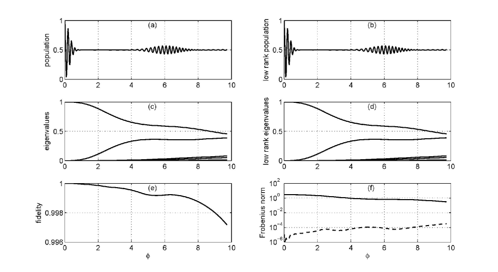
Figures 1, 2 and 3 show that ranks $m\geq 4$ ensure a fidelity higher than $98\%$ over the interval of simulation, and that the fidelity increases with the rank. This is corroborated by the fact that, for $m=4$ and $m=6$, the Frobenius norm of $\dot{\rho}_{\perp}$ is always less than $1\%$ of the Frobenius norm of $\dot{\rho}$. We recall that the fidelity between two density operators $\rho_{a}$ and $\rho_{b}$ is defined by $\text{Tr}\left(\sqrt{\sqrt{\rho_{a}}\rho_{b}\sqrt{\rho_{a}}}\right).$

Figure 1: Oscillation revival for $N_{a}=1$ and a coherent initial field with $\bar{n}=15$ photons; numerical solutions of original Lindblad master equation (1) and of the rank 2 approximation (7,8) with the adimensionalized time $\phi=\Omega_{0}t/2\sqrt{\bar{n}}$; (a) and (b) correspond to the excited atomic populations; (c) and (d) show the first $2$ eigenvalues; (e) is the fidelity between the Lindblad solution and the rank 2 solution; in (f) the solid and dashed curves correspond respectively to the Frobenius norms of $\dot{\rho}$ and $\dot{\rho}_{\perp}$ as explained in (18).

Figure 2: Oscillation revival for $N_{a}=1$ and a coherent initial field with $\bar{n}=15$ photons; numerical solutions of original Lindblad master equation (1) and of the rank 4 approximation (7,8) with the adimensionalized time $\phi=\Omega_{0}t/2\sqrt{\bar{n}}$; (a) and (b) correspond to the excited atomic populations; (c) and (d) show the first $4$ eigenvalues; (e) is the fidelity between the Lindblad solution and the rank 4 solution; in (f) the solid and dashed curves correspond respectively to the Frobenius norms of $\dot{\rho}$ and $\dot{\rho}_{\perp}$ as explained in (18).

Figure 3: Oscillation revival for $N_{a}=1$ and a coherent initial field with $\bar{n}=15$ photons; numerical solutions of original Lindblad master equation (1) and of the rank 6 approximation (7,8) with the adimensionalized time $\phi=\Omega_{0}t/2\sqrt{\bar{n}}$; (a) and (b) correspond to the excited atomic populations; (c) and (d) show the first $6$ eigenvalues; (e) is the fidelity between the Lindblad solution and the rank 6 solution; in (f) the solid and dashed curves correspond respectively to the Frobenius norms of $\dot{\rho}$ and $\dot{\rho}_{\perp}$ as explained in (18).

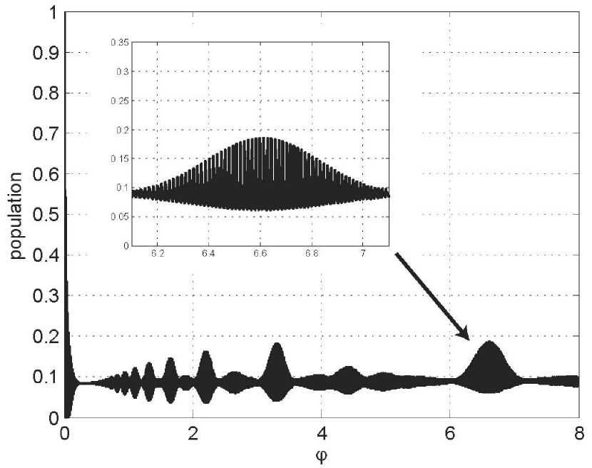
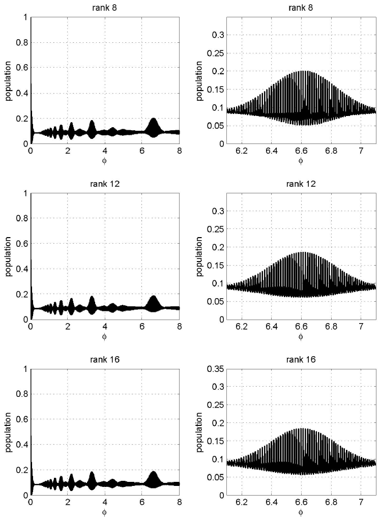
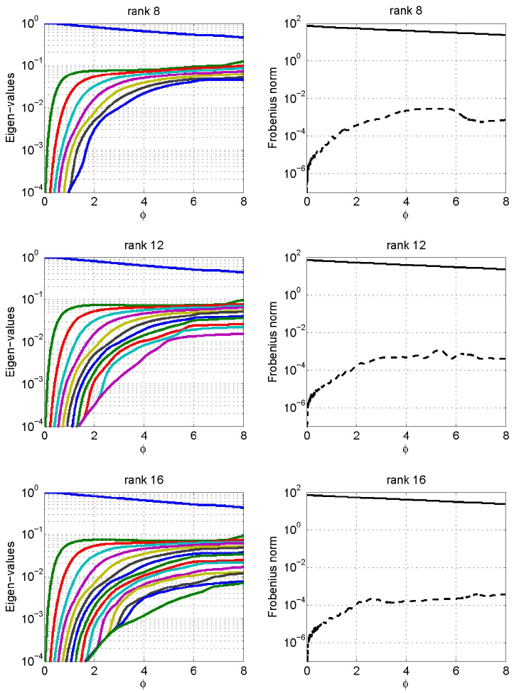
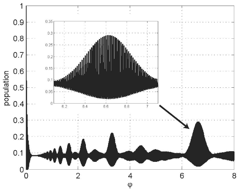
For $N_{a}=50$ atoms initially in the same excited state and a field initially in a coherent state with $\bar{n}=200$ photons a direct numerical integration of the Lindblad master equation (19), when $\kappa>0$, is impossible on the limited computing facilities we have access to. The size $n$ of any finite dimensional approximation of $\rho$ by an $n\times n$ matrix necessarily exceeds $10000$. For the purpose of validating our reduced model, we therefore proceed otherwise. With a truncation to $300$ photons ($n=51\times 301$), we report here two simulations. On Figure 4, we show a reference simulation that is a simulation of the exact Schrödinger equation: the parameter $\kappa$ in (19) is put to zero. The complete revival is maximum. On Figure 5, we simulate our reduced model, based on (7,8) with rank $m=12$, for the parameter value $\kappa=\log(2)\Omega_{0}/(4\pi\bar{n}^{3/2})$. This specific choice of $\kappa>0$ corresponds to a theoretical reduction by a factor 2 of the complete revival appearing at the adimensionalized time $\phi=\Omega_{0}t/2\sqrt{\bar{n}}=2\pi$ as predicted by the formula (45) of [8]. Our simulation is performed with the numerical scheme described in Section 3 with a timestep $\delta t=1/(\Omega_{0}\sqrt{\bar{n}}N_{a})$. Comparing Figure 5 to Figure 4, we recover numerically that the revival amplitude around $\phi=2\pi$ is indeed reduced by a factor $2$. We have also compared in figures 6 and 7 rank $m=12$ with rank $m=8$ and rank $m=16$ approximations. On figure 6 we see that increasing the rank $m$ to 16 does not change the revival amplitude whereas decreasing the rank $m$ to 8 yields a slightly larger revival. On figure 7 we observe that the largest 8 eigenvalues in rank $m=12$ and rank $m=16$ simulations almost coincide with the 8 eigenvalues of rank $m=8$ simulations. This clearly validates our reduced model. To complete this validation, we have checked that smaller timestep and an higher rank $m=20$ do not significantly change the numerical results. For completeness, we mention that the large scale numerical results of Figures 4 and 5 come from computations performed using a simple Matlab code available upon request from the second author. The computations were executed on a Dell Precision M4400 computer equipped with Intel(R) Core(TM) duo CPU T9600 at 2.80GHz with 8.00 Go RAM. The rank $m=12$ simulation of Figure 5 typically takes about 24 hours.

Figure 4: Oscillation revival for $N_{a}=50$ and a coherent initial field with $\bar{n}=200$ photons; evolution with the adimensionalized time $\phi=\Omega_{0}t/2\sqrt{\bar{n}}$ of the excited atomic population (all atoms in the same excited state); numerical solution to the Schrödinger equation (19) with $\kappa=0$.

Figure 5: Oscillation revival for $N_{a}=50$ and a coherent initial field with $\bar{n}=200$ photons; numerical solution of rank $m=12$ approximation (7,8); we show the excited atomic population (all atoms in the same excited state) versus the adimensionalized time $\phi=\Omega_{0}t/2\sqrt{\bar{n}}$; the parameter $\kappa=\log(2)\Omega_{0}/(4\pi\bar{n}^{3/2})$ is adjusted according to [8] in order to get a reduction by a factor $2$ of the revival oscillations around $\phi=2\pi$. That reduction is indeed observed numerically.

Figure 6: Oscillation revival for $N_{a}=50$ and a coherent initial field with $\bar{n}=200$ photons; numerical solution of rank $m=8,12,16$ approximations (7,8); we show the excited atomic population (all atoms in the same excited state) versus the adimensionalized time $\phi=\Omega_{0}t/2\sqrt{\bar{n}}$; the parameter $\kappa=\log(2)\Omega_{0}/(4\pi\bar{n}^{3/2})$ is adjusted according to [8] in order to get a reduction by a factor $2$ of the revival oscillations around $\phi=2\pi$.

Figure 7: Oscillation revival for $N_{a}=50$ and a coherent initial field with $\bar{n}=200$ photons; numerical solution of rank $m=8,12,16$ approximations (7,8); left column eigenvalues of the approximate density matrices versus the adimensionalized time $\phi=\Omega_{0}t/2\sqrt{\bar{n}}$; right column Frobenius norms of $\dot{\rho}$ (solid line) and $\dot{\rho}_{\perp}$ (dashed line) as explained in (18); the other simulations parameters are identical to figure 6.

5 Conclusion

For the numerical integration of high dimensional open quantum systems, we have proposed an approximation approach based on an orthogonal projection onto the set of rank $m$ density matrices. A numerical integration scheme of the system of equations obtained for the reduced, low-rank model has been suggested. Its derivation has been specifically adapted to the situation where the Hamiltonian evolution is must faster than the decoherence evolution. Other situations could be similarly investigated. The scheme has been implemented and tested on oscillation revivals of atoms interacting resonantly with a slightly damped coherent quantized field. The results obtained show the good quality of the approximation, along with an evident significant speed-up with respect to the direct simulation of the full system. Although definite conclusions are yet to be obtained on cases of much larger sizes and extensive comparisons with the classically employed Monte-Carlo approaches are yet to be performed, the satisfactory results obtained to date show the promising nature of the approach. We additionally note that the strategy of approximation developed here is not restricted to open quantum systems. As shown in the appendix, it can be easily adapted to deal with matrix Riccati equations appearing in Kalman filtering, learning and data fusion problems.

Appendix A The Low-rank differential Riccati equation

This appendix relies on an adaptation of the lifting method used in [1]. We compute here the lift of the orthogonal projection onto the rank $m$ covariance matrices of the vector-field defined by the matrix Riccati equation.

We consider the simplest situation: the state $x\in{\mathbb{R}}^{n}$ and output $y\in{\mathbb{R}}^{p}$ are related by the stochastic differential equations ($dw\in{\mathbb{R}}^{n}$ and $d\eta\in{\mathbb{R}}^{d}$ are vectors whose components are independent Wiener processes of standard deviation $1$)

$$dx=Ax\leavevmode\nobreak\ dt+G\leavevmode\nobreak\ dw\quad\text{and}\quad dy=C\leavevmode\nobreak\ dx+H\leavevmode\nobreak\ d\eta$$

where $A$, $G$, $C$ and $H$ are respectively $n\times n$, $n\times n$, $p\times n$ and $p\times p$ matrices with real entries. When $H$ is invertible, the computation of the best estimate of $x$ at $t$ knowing the past values of the output $y$ relies on the computation of the conditional state-error covariance matrix $P$ solution to the Riccati matrix equation

$$\frac{d}{dt}P=AP+PA^{T}+GG^{T}-PC^{T}(HH^{T})^{-1}CP$$ (20)

where ^T stands for transpose. The symmetric $n\times n$ matrix $P$ is non-negative.

When $G=0$, this Riccati equation is rank preserving. It defines then a vector field on the sub-manifold of rank $m<n$ covariance matrices among the symmetric $n\times n$ matrices with real entries and equipped with the Frobenius scalar product. This sub-manifold denoted by $\mathcal{P}_{m}$ admits the over-parameterization

$$(O,R)\mapsto ORO^{T}=P$$

where $O$ belongs to the set of $n\times m$ orthogonal matrices ($O^{T}O={\mathbb{I}}_{m}$) and $R$ is $m\times m$, positive definite and symmetric. We will prove here that the analogue of (4) and (5) reads:

$$\frac{d}{dt}O =\Omega O+({\mathbb{I}}_{n}-OO^{T})\big{(}(A-\Omega)O+GG^{T}OR^{-1}\big{)}$$ (21)

$$\frac{d}{dt}R =O^{T}(A-\Omega)OR+RO^{T}(A^{T}+\Omega)O+O^{T}GG^{T}O-RO^{T}C^{T}(HH^{T})^{-1}COR$$ (22)

where $\Omega$ is an arbitrary skew-symmetric $n\times n$ matrix ($\Omega^{T}=-\Omega$) playing the role of gauge degrees of freedom. The matrix $\Omega$ could possibly depend on $t$, $O$ or $R$. With $\Omega=0$ and $G=0$ we recover the lift given in [1]:

$$\frac{d}{dt}O=({\mathbb{I}}_{n}-OO^{T})AO,\quad\frac{d}{dt}R=O^{T}AOR+RO^{T}AO-RO^{T}C(HH^{T})^{-1}COR.$$

Notice that we can adapt the discretization strategy used for (4) and (5) to get with a proper choice of the gauge matrix $\Omega$ an efficient numerical scheme. Let us conclude by proving that (21) and (22) correspond to a lift of the orthogonal projection onto $\mathcal{P}_{m}$ of the vector-field defined by (20).

Take $P=ORO^{T}$ a rank $m$ covariance matrix. The tangent space at $P$ to $\mathcal{P}_{m}$ is parameterized by $\delta ORO^{T}+O\delta RO^{T}+OR\delta O^{T}$ where $\delta O=\omega O$ and $\delta R=\xi$ are arbitrary variations of $O$ and $R$ associated to any $\omega$ and $\xi$, skew-symmetric $n\times n$ and symmetric $m\times m$ matrices. The orthogonal projection of $\frac{d}{dt}P$ given by (20) onto this tangent space is associated to $\omega$ and $\xi$ minimizing the Frobenius distance between $\delta ORO^{T}+O\delta RO^{T}+OR\delta O^{T}$ and $AP+PA^{T}+GG^{T}-PC^{T}(HH^{T})^{-1}CP$. This means that the skew-symmetric matrix $\omega$ and the symmetric matrix $\xi$ minimize

$$\text{Tr}\left(\left(AP+PA^{T}+GG^{T}-PC^{T}(HH^{T})^{-1}CP-(\omega P-P\omega+O\xi O^{T})\right)^{2}\right).$$

The first order stationary conditions characterizing $\omega$ and $\xi$ read

$$0 =O^{T}\big{(}AP+PA^{T}+GG^{T}-PC^{T}(HH^{T})^{-1}CP-(\omega P-P\omega+O\xi O^{T})\big{)}O$$

$$0 =\Big{[}P\quad,\quad AP+PA^{T}+GG^{T}-PC^{T}(HH^{T})^{-1}CP-(\omega P-P\omega+O\xi O^{T})\Big{]}.$$

Since $O^{T}O={\mathbb{I}}_{m}$ we have

$$\xi=O^{T}\big{(}AP+PA^{T}+GG^{T}-PC^{T}(HH^{T})^{-1}CP-\omega P+P\omega)\big{)}O$$ (23)

and thus $\omega$ is solution to the following matrix equation

$$({\mathbb{I}}_{n}-OO^{T})\big{(}AP+GG^{T}-\omega P\big{)}P=P\big{(}PA^{T}+GG^{T}+P\omega\big{)}({\mathbb{I}}_{n}-OO^{T})$$

obtained after some manipulations using $O^{T}O={\mathbb{I}}_{m}$ and $P({\mathbb{I}}_{n}-OO^{T})=({\mathbb{I}}_{n}-OO^{T})P=0$ This matrix equation admits the following general solution

$$\omega=({\mathbb{I}}_{n}-OO^{T})\big{(}AO+GG^{T}OR^{-1}\big{)}O^{T}-O\big{(}O^{T}A^{T}+R^{-1}O^{T}GG^{T}\big{)}({\mathbb{I}}_{n}-OO^{T})\\ +OO^{T}\Omega OO^{T}+({\mathbb{I}}_{n}-OO^{T})\Omega({\mathbb{I}}_{n}-OO^{T})$$ (24)

where $\Omega$ is an arbitrary skew-symmetric matrix. We get (21) since

$$\omega O=\Omega O+({\mathbb{I}}_{n}-OO^{T})\big{(}(A-\Omega)O+GG^{T}OR^{-1}\big{)}.$$

To get (22) we take $\omega$ given by (24) and insert it into (23).

References

• [1] S. Bonnabel and R. Sepulchre. Matrix Information Geometry, chapter The Geometry of Low-Rank Kalman Filters, pages 53–68. Springer, 2012. Preliminary version: arXiv:1203.4049v1.
• [2] J. Dalibard, Y. Castion, and K. Mølmer. Wave-function approach to dissipative processes in quantum optics. Phys. Rev. Lett., 68(5):580–583, 1992.
• [3] J. Gea-Banacloche. Atom- and field-state evolution in the Jaynes-Cummings model for large initial fields. Phys. Rev. A, 44:5913, 1991.
• [4] R. van Handel and H. Mabuchi. Quantum projection filter for a highly nonlinear model in cavity qed. Journal of Optics B: Quantum and Semiclassical Optics, 7(10):S226, 2005.
• [5] S. Haroche and J.M. Raimond. Exploring the Quantum: Atoms, Cavities and Photons. Oxford University Press, 2006.
• [6] Ch. Lubich. From quantum to classical molecular dynamics: reduced models and numerical analysis. European Mathematical Society (EMS),Zürich, 2008.
• [7] H. Mabuchi. Derivation of Maxwell-Bloch-type equations by projection of quantum models. Phys. Rev. A, 78:015801, Jul 2008.
• [8] T. Meunier, A. Le Diffon, C. Ruef, P. Degiovanni, and J.-M. Raimond. Entanglement and decoherence of N atoms and a mesoscopic field in a cavity. Phys. Rev. A, 74:033802, 2006.
• [9] K. Mølmer, Y. Castin, and J. Dalibard. Monte Carlo wave-function method in quantum optics. J. Opt. Soc. Am. B, 10:512–537, 1993.