New Generation of the Monte Carlo Shell Model for the K Computer Era

Abstract

We present a newly enhanced version of the Monte Carlo Shell Model method by incorporating the conjugate gradient method and energy-variance extrapolation. This new method enables us to perform large-scale shell-model calculations that the direct diagonalization method cannot reach. This new generation framework of the MCSM provides us with a powerful tool to perform most-advanced large-scale shell-model calculations on current massively parallel computers such as the K computer. We discuss the validity of this method in ab initio calculations of light nuclei, and propose a new method to describe the intrinsic wave function in terms of the shell-model picture. We also apply this new MCSM to the study of neutron-rich Cr and Ni isotopes using the conventional shell-model calculations with an inert ⁴⁰Ca core and discuss how the magicity of $N=28,40,50$ remains or is broken.

1 Introduction

The understanding of the structure of all nuclei from the first principle, called usually the ab initio nuclear calculation, is one of the ultimate goals in nuclear theory. For this purpose, one usually starts with the nucleon degree of freedom, i.e., protons and neutrons as the building block of a nucleus, assuming the free (or bare) nucleon-nucleon force to be the interaction between nucleons. Recent ab initio calculations often include not only the two-nucleon force but also the three-nucleon force which is specific to the interaction between composite particles like nucleons. Several ab initio methods have been proposed, and their accuracy has been investigated in great detail, for instance, in terms of the binding energy of the four-nucleon system [1]. It remains, however, rather difficult or infeasible to go beyond systems with $A\gtrsim 12$, where $A$ is the number of nucleons. This is largely due to strong nucleon-nucleon correlations that requires a large number of single-particle states to be included for the description of many-body states in ground states or low excited states. Although this problem can be resolved to a certain extent by using effective interactions based on various renormalization techniques, the number of many-body states to be included remains prohibitively large in most cases, and increases exponentially with the nucleon number. In this paper, we present a new version of the Monte Carlo shell model (MCSM), demonstrating how it can contribute to ab initio nuclear calculation as well as to conventional but quite huge shell model calculations.

The nuclear shell model has been known to be successful in describing the structure of atomic nuclei based on nuclear forces. It dates back to 1949 when Mayer and Jensen discovered the magic numbers as a consequence of a mean potential including the spin-orbit coupling [2]. While the original concept of the shell model of Mayer and Jensen is basically an independent particle picture, the concept has been modified and extended significantly over decades since then. The modern shell model uses a sufficiently large number of many-body basis states which are superposed utilizing properly constructed effective interactions so as to provide us with accurate many-body eigenstates. The many-body basis state is a Slater determinant usually with single-particle states taken from a harmonic oscillator potential.

In conventional shell-model calculations, an inert core is assumed: all single-particle states below a given magic number are completely occupied, forming a closed shell. Single-particle states between this magic number and the next magic number constitute a valence shell, and nucleons in this shell are called valence nucleons. In the conventional shell model, only valence nucleons are activated. The single-particle states of activated nucleons in the shell-model calculation are called the model space. The model space is a concept for calculation, and is the same as some valence space in many cases. But, in other cases, the model space can be taken wider or smaller than the relevant valence shell depending on some interest or limitation. We thus distinguish model space from valence shell hereafter. Note that the model space is a more computational concept.

An effective interaction is obtained for valence nucleons, and is defined for each model space. Effects from the inert core, those from virtual excitations from the inert core and those from virtual excitations to states above the model space are assumed to all be incorporated into this effective interaction by renormalizing it appropriately. This can be a very important issue, but the conventional shell model assumes that there is such an interaction, while its determination can be phenomenological.

It has been shown that many nuclear properties with $8\leq N(Z)\leq 20$ are excellently described with the conventional shell model calculation in the $1s$-$0d$ (model) space (often called the $sd$ shell) [3, 4], and those with $20\leq N(Z)\lesssim 32$ are also quite well described in the $1p$-$0f$ (model) space (often called the $pf$ shell) [5, 6]. Note that the effective interactions used in those calculations are hybrid products of microscopic derivation and empirical adjustments.

While the conventional shell model assumes a relatively limited model space as exemplified above, the same computational procedure is applicable to the ab initio calculation when no inert core is assumed and a large number of single-particle states are taken so that the calculation becomes close to calculations in the whole Hilbert space. Here, we refer to this ab initio method within the shell model as the ab initio shell model, one of which is the no-core shell model (NCSM) [7], a famous model with great success.

Whether the ab initio shell model or the conventional shell model (with a core) is used, all one has to do in computation is to diagonalize a Hamiltonian matrix spanned by all the possible many-body states in a given model space (i.e., single-particle space of activated nucleons). The number of relevant many-body basis states determines the dimension of this matrix. This dimension is often called the shell-model dimension, and causes a serious computational issue as we shall see later. The number of the many-body states is ${}_{N_{p}}C_{n_{p}}\times\,_{N_{n}}C_{n_{n}}$ without symmetry consideration, where $N_{p}$ ($N_{n}$) is the number of proton (neutron) single-particle states taken and $n_{p}$ ($n_{n}$) is the number of protons (neutrons) activated. It roughly increases exponentially with $N_{p}$ (or $N_{n}$) and also with $n_{p}$ (or $n_{n}$). Hence, without even considering the ab initio shell model with a huge number of $N_{p}$ and $N_{n}$, the conventional shell model for heavier nuclei already suffers from the huge dimensionality of the Hamiltonian matrix necessary to tackle the whole nuclear chart because the number of valence orbits ($N_{p}$ or $N_{n}$) increases for heavier nuclei. For instance, the dimension needed for $A\sim 80$ $N=Z$ nuclei is estimated to be $\sim 10^{27}$ without any symmetry consideration [8] when the $1p$-$0f$-$2s$-$1d$-$0g$ orbits are assumed to be the valence shell. Although this number can be reduced by 1-2 orders of magnitude by choosing only the states of the same $J_{z}$ as taken usually (i.e., $M$-scheme calculation), it is still far from the current computational limit of $10^{10-11}$ in the $M$-scheme.

In order to go beyond the computational limit of the shell model, a new method for performing the shell-model calculation named the Monte Carlo shell model (MCSM) has been developed since 1996 [9], guided by the Quantum Monte Carlo Diagonalization method [10]. The MCSM utilizes the idea of the auxiliary field Monte Carlo method that is taken in the Shell Model Monte Carlo method [11], but this method and the MCSM are completely different. The MCSM aims to represent many-body states with a small number of highly selected many-body basis states. In this sense, the MCSM is regarded as an “importance truncation” of the entire many-body space [12]. The basis state should be represented in a compact form (i.e., a wave function with a small number of parameters), it should be able to approximate the nuclear many-body state efficiently, and its matrix elements should be calculated easily. To meet this demand, we usually use deformed Slater determinants, and parity and total angular momentum projection are operated on them if needed. Otherwise, a pair condensed state [13] or a quasi-particle vacuum state, which is used in the Hartree-Fock-Bogoliubov calculation and also taken as the basis state of the VAMPIR (abbr. for Variational After Mean field Projection In Realistic model spaces) method [14], is a good candidate when required. Note that the VAMPIR method has been developed with more emphasis on calculating the energy spectra rather than improving the energy of a specified state. The MCSM basis states are added one by one, and each basis state to be added is selected among many candidate Slater determinants generated stochastically so that the energy of the state under consideration can be as low as possible. This step is repeated until the energy converges sufficiently. Thus, this original MCSM is characterized as “stochastic” in terms of the method of basis variation, and as “sequential” in terms of the procedure of basis variation.

From the computational point of view, the MCSM has an advantage over the conventional diagonalization method in tolerance to the increase of the model space and the particles. When it is assumed that the number of basis states needed in a MCSM wave function is fixed, the total computational cost is scaled by the cost of each Hamiltonian matrix element. This is roughly proportional to $(N_{sp})^{\alpha}$ with $\alpha\sim 3$-$4$ in the case of $N_{sp}=N_{p}=N_{n}$, being much milder than the exponential increase. This advantage had enabled us to perform the full $pf$-shell calculation in ⁵⁶Ni (with $\sim 10^{9}$ $M$-scheme dimension) with good accuracy [15] several years before the exact diagonalization was carried out [14]. See the review paper [12] for more details of early achievements.

Recently, the computational environment has been changing rapidly. The number of available CPU cores is expanding to be typically in the range of tens of thousands for the world leading supercomputers as compared to a few tens to hundreds of CPU cores used in the early MCSM calculations. The K computer will contain more than 700,000 cores upon its completion in the autumn of 2012. This situation has strongly motivated us to renew the MCSM method to be suitable using up-to-date massive parallel computers, in addition to wider applications including ab initio shell model calculations. Since 2009, we have developed a new MCSM package, which includes not only renewed code, but also a novel methodology and numerical algorithm [16]. Among the methodological advancements, the most important is the introduction of the energy-variance extrapolation method [17]. In the original MCSM, the energy of a many-body state is evaluated directly from the energy expectation value of the MCSM wave function, which must be higher than the exact solution. It was quite hard to know the difference between this value and the exact value. The energy-variance extrapolation method serves as a powerful tool to pin down accurately the exact solution from a series of approximated solutions. Another methodological change is incorporating a variational aspect into the MCSM by varying the basis state, which enhances the lowering of calculated energy values. Equipped with the variational-type improvement, the MCSM is now characterized as “deterministic” in terms of the method of basis variation. Thus, keeping the original idea, the present MCSM, associated with several advancements, can be regarded as a new generation.

In this paper, we review the outline of the new-generation MCSM and show some of its earliest applications that were not feasible with the original MCSM. This paper is organized as follows. In Sect. 2, the outline of the new-generation MCSM and its feasibility are presented. We also discuss the adaptability of the MCSM to massively parallel supercomputers. In Sect. 3, application to the ab initio shell model is demonstrated. Along with numerical success, the intrinsic shape and the clustering of light nuclei are also discussed with the MCSM wave function. In Sect. 4, application to the neutron-rich chromium and nickel isotopes is presented as a case of medium-heavy mass nuclei. This region is being intensively studied in radioactive isotope facilities over the world, and also challenges nuclear models because several shapes coexist and are mixed, which results in the rapid change of the dominant shape over the isotopes. In Sect. 5, we summarize this paper and give an outlook and future perspective of the MCSM toward the launch of the K computer.

We note here that many new features may appear in the structure of exotic nuclei, because unbalanced numbers of protons and neutrons may create situations where unknown or little known aspects of nuclear forces become visible and produce large impacts. The shell evolution due to the tensor force [18, 19, 20] and the three-body force [21] are some examples. Note that the shell evolution explains basic trends of single-particle properties and one needs comprehensive calculations to obtain physical quantities and look into correlations in depth. The exploration of such unknown features need theoretical framework directly linked to nuclear forces, and we expect a large contribution from the new generation of MCSM.

2 Outline of the new-generation Monte Carlo shell model

The new-generation MCSM can be divided roughly into two stages: the variational procedure to obtain the approximated wave function and the energy-variance extrapolation utilizing the obtained wave function. We briefly describe these two parts in Sects. 2.2 and 2.3, respectively. The shell-model Hamiltonian and the form of the variational wave function used in the MCSM is shown in Sect.2.1. The additional improvement to make the extrapolation procedure stable is demonstrated in Sect. 2.4. The numerical aspects of the framework mainly for massively parallel computation are discussed in Sect. 2.5.

2.1 Shell-model Hamiltonian and variational wave function

In conventional nuclear shell-model calculations assuming an inert core, we use a general two-body interaction:

$$H=H^{(1)}+H^{(2)}=\sum_{i}t_{i}c^{\dagger}_{i}c_{i}+\sum_{i<j,k<l}v_{ijkl}c^{\dagger}_{i}c^{\dagger}_{j}c_{l}c_{k},$$ (1)

where $c^{\dagger}_{i}$ denotes a creation operator of single particle state $i$. $H^{(1)}$ is a one-body Hamiltonian with single-particle energies $t_{i}$, and $H^{(2)}$ is a two-body interaction which has parity and rotational symmetry and is represented by so-called Two-Body Matrix Elements (TBMEs) [22].

In the case of ab initio shell-model calculations, the Hamiltonian is taken as

$$H=T-T_{\rm CM}+V=\sum_{ij}t_{ij}c^{\dagger}_{i}c_{j}+\sum_{i<j,k<l}v_{ijkl}c^{\dagger}_{i}c^{\dagger}_{j}c_{l}c_{k},$$ (2)

where $T$ and $T_{\rm CM}$ are the total kinetic energy and the kinetic energy of the center-of-mass motion, respectively. Note that $T_{\rm CM}$ has both one-body and two-body components. The $V$ represents two-nucleon interaction, e.g., the JISP16 interaction [24] in Sect. 3. In this work, because we do not treat explicitly three-nucleon forces, both the Hamiltonians of these two kinds of shell-model calculations consist of one-body and two-body interactions.

If necessary, the removal of spurious center-of-mass motion can be done by utilizing the prescription of Gloeckner and Lawson [25] to suppress the contamination of the center-of-mass motion. In this prescription the Hamiltonian to be diagonalized is replaced by

$$H^{\prime}=H+\beta_{\rm cm}H_{\rm cm}$$ (3)

with $H_{\rm cm}$ being defined as

$$H_{\rm cm}=\frac{\bf P^{2}}{2AM}+\frac{1}{2}MA\omega^{2}{\bf R}^{2}-\frac{3}{2}\hbar\omega,$$ (4)

where $\bf R$ and $\bf P$ are the position and momentum of the center of mass. By taking $\beta_{\rm cm}$ large enough, $\langle H_{\rm cm}\rangle$ is suppressed as a small value.

In the framework of the MCSM, the approximated wave function is written as a linear combination of angular-momentum- and parity-projected Slater determinants,

$$|\Psi_{N_{b}}\rangle=\sum_{n=1}^{N_{b}}\sum_{K=-I}^{I}f^{(N_{b})}_{n,K}P^{I\pi}_{MK}|\phi_{n}\rangle,$$ (5)

where $N_{b}$ is the number of the Slater-determinant basis states. The $P^{I\pi}_{MK}$ operator is the angular-momentum and parity projector defined as

$$P^{I\pi}_{MK}=\frac{1+\pi\Pi}{2}\frac{2I+1}{8\pi^{2}}\int d\Omega\ {D^{I}_{MK}}^{*}(\Omega)e^{i\alpha J_{z}}e^{i\beta J_{y}}e^{i\gamma J_{z}},$$ (6)

where $\Omega\equiv(\alpha,\beta,\gamma)$ are the Euler angles and $D^{I}_{MK}(\Omega)$ denotes Wigner’s $D$-function. $\Pi$ stands for the parity transformation. Each $|\phi_{n}\rangle$ is a deformed Slater determinant defined in Eq.(11). The coefficients $f^{(N_{b})}_{n,K}$ are determined by the diagonalization of the Hamiltonian matrix in the subspace spanned by the projected Slater determinants, $P^{I\pi}_{MK}|\phi_{n}\rangle$ with $-I\leq K\leq I$ and $1\leq n\leq N_{b}$. This diagonalization also determines the energy, $E_{N_{b}}\equiv\langle\Psi_{N_{b}}|H|\Psi_{N_{b}}\rangle$, as a function of $N_{b}$. Note that the dimension of the subspace is $(2I+1)N_{b}$, not $N_{b}$. The Slater determinant basis, $D^{(n)}$, is given by variational calculation to minimize $E_{N_{b}=n}$. We increase $N_{b}$ until $E_{N_{b}}$ converges enough, or the extrapolated energy converges. The strategy of this variational calculation will be discussed in the next subsection.

2.2 Variational procedure

In this section, we discuss the efficient process for the determination of $D^{(n)}$ in Eq.(11) to minimize $E_{N_{b}}$ and the history of its developments in this section. In the original MCSM calculation, the basis states are selected from many candidates generated stochastically utilizing the auxiliary-field Monte Carlo technique, the detail of which was discussed in Ref. ppnp_mcsm. In order to determine $D^{(n)}$ in Eq.(5) efficiently, M. Honma et al. introduced the few-dimensional basis approximation [26], in which they adopted the steepest gradient method. It succeeded in estimating the energy of $pf$-shell nuclei with a relatively small number of bases, however, the direction of the gradient is not necessarily the most efficient choice to reach the local minimum and it is practically difficult to control the step width in the gradient direction. Mainly because of this problem, the number of basis states was limited to be rather small ($N_{b}\simeq 30$) compared to that in the MCSM ($N_{b}\simeq 100$). On the other hand, W. Schmid et al. adopted the quasi-Newton method for energy minimization in the VAMPIR approximation to obtain the optimized quasi-particle vacua as basis states [27]. G. Puddu demonstrated that the quasi-Newton method works also in the Slater determinant bases. In the quasi-Newton method, the step width is automatically determined to minimize the energy along the modified gradient direction [28, 29]. As a result, the step width is relatively large in early steps of the quasi-Newton procedure along the sophisticated gradient direction so that the additional basis state has sufficiently linearly independent component of the other basis states.

In the present work, we adopt the conjugate gradient (CG) method [30, 31], which also includes the linear minimization in the modified gradient direction. In comparison to the quasi-Newton method, the CG method is expected to be advantageous to save memory usage and improve computational efficiency for parallel computation because a large Hessian matrix is utilized in the quasi-Newton method, which is not used in the CG method. Note that the energy of the linear combination of projected Slater determinants is optimized, not that of the unprojected Slater determinants. In this sense, this variational procedure is “variation after projection and configuration mixing”.

We proposed the following four steps to optimize the parameters of deformed Slater determinants:

1. Monte Carlo sampling utilizing auxiliary field technique (original MCSM),

2. Sequential optimization for each basis state (SCG),

3. Refinement process of each basis states repeatedly (refinement),

4. Full (simultaneous) optimization of all basis states (FCG).

In the first step, we perform the original MCSM procedure to obtain the approximated wave function, which can be used as an initial state of the CG process. The detail of the original MCSM is not discussed here, but in Ref. ppnp_mcsm. In Refs. ppnp_mcsm, mcsm_extrap. we select the best basis states from an order of 1000 candidates, which is generated stochastically. However, the necessary number of candidates can be far suppressed if we proceed to the next step.

In the second step, called the SCG method, we perform a variational calculation, with variational parameters being $D^{(i)}$, sequentially by minimizing the $E_{i}$ without changing the other bases, $D^{(1)},D^{(2)},...D^{(i-1)}$, which were already fixed. In other words, we perform variational calculations with a set of variational parameters, $D^{(i)}$, sequentially. We increase the number of basis states, $N_{b}$, until the energy reaches sufficient convergence.

In the third step which is called the refinement process, we take an initial state from the result of the SCG calculation. In the SCG calculation, the $D^{(1)}$ is not the best optimized parameters to minimize $E_{N_{b}}$, since $D^{(1)}$ is determined to minimize $E_{1}$. Then, we first fix the number of basis states, $N_{m}$, and restart to minimize the energy $E_{N_{m}}$ by the CG method to optimize each basis state from $D^{(1)}$ to $D^{(N_{m})}$, one by one. We iterate a few times to perform a routine of the CG process for all basis states one by one to get a better energy calculation.

In the fourth step called the FCG, we fix $N_{m}$ at the beginning, and determine all coefficients $D^{(N_{b})}$ with $1\leq N_{b}\leq N_{m}$ by minimizing the $E_{N_{m}}$ at once. In other words, we perform variational calculation with a set of all variational parameters, $D^{(N_{b})}$, simultaneously to minimize the $E_{N_{m}}$. Its initial state is generated by the refinement process in order to save the amount of computation time. In principle, the FCG yields the closest energy to the exact one within a fixed number of basis states, $N_{m}$, and the refinement process also reaches the energy provided by the FCG with a large number of iterations. The refinement process needs a far smaller amount of time than that in the FCG, and provides us with an approximation good enough to the solution in the FCG.

Figure 1 shows the convergence pattern of the ground-state energy of ⁷²Ge in $f_{5}pg_{9}$ shell, which consists of the $0f_{7/2}$, $1p_{3/2}$, $1p_{1/2}$, and $0g_{9/2}$ orbits. Its $M$-scheme dimension is very large and amounts to 140,050,484. However, it can be handled by the recent shell-model diagonalization code [32]. The energy eigenvalue $E_{N_{b}}=\langle\Psi_{N_{b}}|H|\Psi_{N_{b}}\rangle$ is plotted against the number of basis states, $N_{b}$. The SCG method attains faster convergence than the original MCSM: the SCG gives the same energy as the original MCSM in almost half the number of basis dimension. The SCG method enables us to compute the energy variance in a smaller amount of the computation time than that of the original MCSM, since the time to compute the energy variance is proportional to $N_{m}(N_{m}+1)/2$.

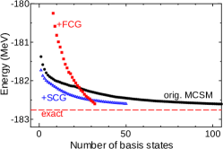
Figure 1: Convergence patterns of the ground-state energy of ⁷²Ge in the $f_{5}pg_{9}$ shell. The circles, open triangles, and squares denote the results of the original MCSM, SCG, and FCG with $N_{m}=32$, respectively.

In the case of the FCG, the number of basis states of the variational wave function is fixed to $N_{m}=32$ and we plot energy expectation values in the subspace spanned by the $N_{b}$ basis states. In the FCG all basis states, $D^{(1)},D^{(2)},...,$ and $D^{(32)}$, are optimized to minimize $E_{32}$, while in the SCG wave function $D^{(1)}$ is optimized to minimize $E_{1}$. Thus, the calculated $E_{1}$ of the FCG is much higher than the $E_{1}$ of the SCG and the $E_{1}$ of the original MCSM. However, $E_{32}$ of the FCG is lower than that of the SCG and the original MCSM, which means the FCG provides us with the best approximation for a fixed number of basis states. Therefore, we should discuss the energy convergence as a function of $N_{m}$ in the FCG, not as a function of $N_{b}$, unlike the case of the SCG.

While the FCG yields the best energy with the fixed $N_{m}$, the FCG iteration needs much computational resources since we have to replace all basis states at every FCG iteration. Which level of the optimization is most efficient in terms of the computation time depends on the property of the objective wave function. For applications, we adopt the original MCSM method and the SCG method in Sect. 3 and the refinement process in Sect. 4.

2.3 Energy-variance extrapolation

Even if the variational procedure works excellently, a small gap between the exact energy eigenvalue and the energy expectation value of the approximated wave function remains. The gap can be removed by extrapolation procedures, which have been studied intensively [33, 34, 35, 36]. Among them, the energy-variance extrapolation method is a general framework for the supplementation of the variational calculation and is rather independent of the form of the approximated wave function. This method has been known in condensed matter physics [37] and was firstly introduced in shell-model calculations with conventional particle-hole truncation by T. Mizusaki and M. Imada [34]. In the present work, we apply this extrapolation method to estimate the exact eigenvalue precisely by utilizing a sequence of the linear combinations of the projected Slater determinants, $|\Psi_{N_{b}}\rangle$ with $1\leq N_{b}\leq N_{m}$, which have been obtained in the variational procedure discussed in Sect.2.2. The major obstacle of the energy-variance extrapolation is the necessity of the computation of the energy variance. Its efficient computation is described in Sect.2.5.

The energy-variance extrapolation method is based on the fact that the energy variance of the exact eigenstate is zero. The energy variance of the approximated wave function is not exactly zero, but rather small and approaches zero as the approximation is improved. In the framework of the energy-variance extrapolation, we draw the energy $E_{N_{b}}=\langle\Psi_{N_{b}}|H|\Psi_{N_{b}}\rangle$ against the energy variance $\langle\Delta H^{2}\rangle_{N_{b}}=\langle\Psi_{N_{b}}|H^{2}|\Psi_{N_{b}}\rangle-E_{N_{b}}^{2}$, the plot of which is called “energy-variance plot”. The variance usually approaches zero as $N_{b}$ increases, as the point in the energy-variance plot approaches the $y$-intercept. Following the idea of Ref.extrap_2ndorder, These points are usually fitted by a first- or second-order polynomial such as

$$E=c_{0}+c_{1}\langle\Delta H^{2}\rangle+c_{2}(\langle\Delta H^{2}\rangle)^{2},$$ (7)

where these coefficients $c_{0}$, $c_{1}$, and $c_{2}$ are determined by least square fit. By extrapolating the fitted curve into the $y$-intercept we obtain the extrapolated energy, namely, $c_{0}$.

In the framework of the present study, the variational procedure discussed in Sect. 2.2 provides us with a sequence of approximated wave functions, which can be utilized in the energy-variance extrapolation method. The SCG procedure provides us with a successive sequence of the wave functions, $|\Psi_{N_{b}}\rangle$ with $1\leq N_{b}\leq N_{m}$, where $N_{m}$ is the maximum of $N_{b}$. For each $N_{b}$, we evaluate the energy $E_{N_{b}}$ and energy variance $\langle\Delta H^{2}\rangle_{N_{b}}$. Here, we demonstrate how the extrapolation method works with ⁵⁶Ni in the $pf$ shell as an example. The effective interaction is the FPD6 interaction [38], which was adopted also in Ref. mcsm_extrap.

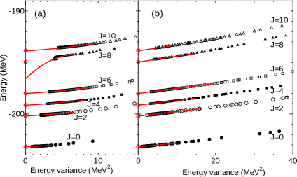
Figure 2: Energy-variance plot for ⁵⁶Ni (a) without reordering, (b) with reordering. The open circles on the $y$-axis denote the exact shell-model energies. See text for details.

Figure 2(a) shows the energy-variance plot of the SCG method for yrast states of ⁵⁶Ni. In this calculation, we take the $K=I$ state only in the angular-momentum projector, namely $f_{n,K}^{(N_{b})}=0$ if $K\neq I$ in Eq.(5), for simplicity. As $N_{b}$ increases the energy-variance point moves smoothly and approaches the $y$-axis or variance zero, except for the $8^{+}$ state. The fitted curves for these points are shown as red solid lines, and they also show smooth behavior. The extrapolated energies, or $y$-intercepts of the fitted curves, agree quite well with the exact ones, which are shown as open circles on the $y$-axis. Especially concerning the ground-state energy, the minimum variance of the approximated wave function is $\langle\Delta H^{2}\rangle_{N_{b}=100}=0.89$MeV², which is smaller and gives a better approximation than the result of the original MCSM, $\langle\Delta H^{2}\rangle_{N_{b}=150}=1.05$MeV² [17], mainly thanks to the introduction of the CG method.

On the other hand, the plot of the $8^{+}$ state shows the anomalous behavior, in which the energy decreases when increasing the number of basis states but the variance does not decrease at $\langle\Delta H^{2}\rangle\simeq 4$MeV². As a result, the simple extrapolation method apparently fails. A straightforward solution to this failure is to increase $N_{b}$ until the extrapolation method works, and it is shown in Ref. okinawa_shimizu. However, in other cases, it might be difficult due to the increase of computation time. We discuss another remedy for such cases in the following section.

2.4 Reordering technique to improve the energy-variance extrapolation

The anomalous behavior can be removed by the reordering of the basis states [39]. In this section, we demonstrate that the reordering technique makes the energy-variance extrapolation stable and avoids the difficulty of an anomalous kink such as the $8^{+}_{1}$ state of ⁵⁶Ni discussed in the previous subsection.

A sequence of the approximated wave functions, ($|\Psi_{1}\rangle$, $|\Psi_{2}\rangle$, …, $|\Psi_{N_{b}}\rangle$, …, $|\Psi_{N_{m}}\rangle$) is specified by a set of basis states and its order ($|\phi_{1}\rangle$, $|\phi_{2}\rangle$, …, $|\phi_{N_{b}}\rangle$, …, $|\phi_{N_{m}}\rangle$). In the SCG method, the order of the basis states is determined by the variational procedure. However, we can shuffle the order of basis states and make another sequence of the approximated wave functions without additional computational effort. If we assume that the extrapolated value is independent of the order of the basis states, there exists the best order which makes the extrapolation procedure stable. In the reordering method, the order is determined so that the gradient of the curve in the energy-variance plot is as small as possible. The practical algorithm to determine the order is discussed in Ref. shimizu_reordering.

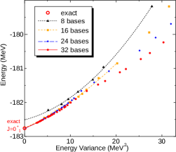
Figure 3: Energy vs. energy variance plot of the ground state energy of ⁷²Ge in the $f_{5}pg_{9}$ shell. The wave functions are provided by the FCG with $N_{m}=8$ (triangles), 16 (squares), 24 (diamonds), and 32 (circles).

Figure 2(b) shows the extrapolation plot with the reordering technique using the same set of the basis states as in Fig. 2(a). In this case, the gradient of the fitted curve is so stable that the points in the energy-variance plot are fitted by a first-order polynomial and the region to be used for the fit is rather broad. In Fig. 2(b), the anomalous behavior of the variance plot of the $8^{+}$ state disappears and the extrapolated value agrees with the exact energy quite well. ⁵⁶Ni is also known to have a shape coexistence feature [40], which is plausible to be the origin of the anomalous behavior of the $8^{+}$ state in Fig. 2(a) like the case of ⁷²Ge discussed in Ref.shimizu_reordering.

We demonstrate another example of the energy-variance extrapolation method combined with the reordering technique in Fig. 3 using the FCG wave functions of ⁷²Ge with the JUN45 effective interaction [41]. In this figure, the energy expectation value of the FCG wave function is plotted as a function of the corresponding energy variance with the basis states being $N_{m}=8,16,24,$ and $32$, and their second-order fitted curves. The order of the basis states in each sequence is determined by the reordering technique[39]. Note that there is no specific order in the FCG procedure because we treat all basis states on an equal footing. The extrapolated energy apparently converges except for $N_{m}=8$. While we show the second-order fit in the figure, even the extrapolated value of the first-order fit agrees well with that of the second-order fit in the case of $N_{m}=32$.

2.5 Computational aspects

The large-scale shell-model calculation is one of the challenging issues for nuclear physics. It is essential to develop a program which runs efficiently on recent supercomputers. Concerning a calculation using a single CPU, we proposed a sophisticated way of efficient computation of the matrix element of non-orthogonal Slater determinants in Ref.mcsm_tuning. Moreover, since the main trend of recent supercomputers favors massively parallel computers, the parallel efficiency is worth discussing for future studies.

In the case of the SCG method, we need to compute the Hamiltonian matrix elements and the gradient vector concerning $D^{(n)}$ of two angular-momentum-, parity-projected Slater determinants. The three-dimensional integral of the Euler angles in Eq.(6) is performed by discretizing each range of the integral into mesh points using the Gauss-Chebyshev quadrature for the $z$-axis rotations and the Gauss-Legendre quadrature for the $y$-axis rotation, which is shown in Eq.(13). The numbers of the mesh points are taken as 26 for the $z$-axis rotation and 16 for the $y$-axis rotation for example. The parity projection is equivalent to two mesh points. The product of these mesh points, which are denoted by $\lambda$ in Eq.(13) give rise to $N_{\rm mesh}=26^{2}\times 16\times 2=21632$ components in evaluating a matrix element in terms of the projected Slater determinants. Since these components can be computed independently, the program was written for massive parallel computation. When we apply the matrix-product technique discussed in Ref.mcsm_tuning with the bunch size $N_{\rm bunch}$ being e.g. 30, we still have the $N_{b}N_{\rm mesh}/N_{\rm bunch}\simeq 721N_{b}$ elements to be computed in parallel.

Figure 4 shows the parallel efficiency of the benchmark calculation of the ground state of ⁶⁴Ge as an example. The model space consists of the $pf$ shell and $g_{9/2}$ orbit and the PFG9B3 effective interaction is used [43]. Its $M$-scheme dimension reaches $1.7\times 10^{14}$, which is far beyond the current limitation of the Lanczos method. The MCSM result of this system was already reported in Refs. mcsm_extrap, shimizu_reordering. This benchmark was performed using the Intel Fortran compiler ver.11.0 [44] on the T2K open Supercomputer at the University of Tokyo [45].

Figure 4: (a) Speedup of the parallel computation of the SCG process in unit of the computation time using 16 CPU cores. The squares, open circles, triangles and filled circles represent the inverses of computation times of the variational process to obtain 1st, 4th, 16th, and 32nd basis states respectively. The solid line shows ideal scaling to guide the eyes. (b) Speedup of the parallel computation of the energy variance. The squares, triangles, and circles represent the inverses of computation times of 1, 4, and 8 basis states, respectively.

Figure 4 (a) shows the performance gain of the parallel computation of the SCG process to determine the 1st, 4th, 8th, 16th, and 32nd basis states respectively. Although the parallel efficiency for calculating the first basis state is not good because of the small amount of computation, the efficiency for the 32nd basis state with 2048 CPU cores reaches 82% of that with 16 cores.

We calculate the energy variance using the formula shown in Appx.A[17]. Because the two-body matrix elements in the $M$-scheme, $v_{ijkl}$, are sparse due to the symmetry which the Hamiltonian has, we store in memory only non-zero matrix elements in block-diagonal form by treating $v_{(ij),(kl)}$ as a rank-2 matrix with indices $(ij)$ and $(kl)$. Thus, we can compute the energy variance efficiently, and the detail of the practical computation is written in Appx.A. In a similar manner to the case of the variational process, we compute the energy variance by dividing the whole computation into matrix elements which are moreover divided into each mesh point of Eq.(6), resulting in $N_{b}(N_{b}+1)\times N_{\rm mesh}$ independent components to be computed in parallel. In addition, we do not need an iterative process like the CG method, and therefore a small amount of network communication appears only at the beginning and at the end of the computation. Thus the performance scaling of the parallel computation seems perfect at $N_{b}\geq 4$, which is shown in Fig. 4(b).

In practice, it took totally 807 seconds to obtain an SCG wave function of ⁶⁴Ge $0^{+}_{1}$ state with 32 basis states, and it took 588 seconds to compute the energy variance of this SCG wave function using 2048 CPU cores.

3 Application of the MCSM to the ab initio shell model

In this section we focus on the latest application of the MCSM to the ab initio shell model calculations, which has become feasible recently with the aid of major development of the MCSM algorithm discussed in Sect. 2 and also a remarkable growth in the computational power of state-of-the-art supercomputers. First, the no-core shell model (NCSM) and its variants are briefly reviewed. The limitation of the NCSM and the motivation for the application of the MCSM to the ab initio no-core Full Configuration Interaction (FCI) approach are further discussed here. Then, the current status of the benchmarks in the no-core MCSM is referred to based on the results mostly from Ref. [46]. Finally our challenge to visualize the intrinsic states constructed by superpositioned non-orthogonal Slater determinants is also demonstrated.

3.1 Ab initio shell models

One of the major challenges in nuclear theory is to understand nuclear structure and reactions from ab initio methods. Ab initio calculations for nuclear many-body systems beyond $A=4$ have recently become feasible due to the rapid evolution of computational technologies these days. In ab initio approaches for the nuclear structure calculations, all the nucleons constituting the nucleus are considered as the fundamental degrees of freedom and the bare/effective interactions based on realistic nuclear forces are adopted. As for bare two- and three-nucleon interactions, the phase-shift equivalent family of two-nucleon interactions, derived from the meson-exchange theory and chiral Effective Field Theory, in addition to three-nucleon interactions [47, 48, 49, 50, 51] is usually used.

Ab initio NCSM has been emerging for about a decade and is now available for the study of nuclear structure and reactions in the $p$-shell nuclei [7]. Unlike the conventional shell model with a core, the NCSM does not assume an inert core just like the name itself implies and treats all the nucleons composing the nucleus on an equal footing. The NCSM is thus said to be one of the ab initio approaches along with the Green’s Function Monte Carlo [52] and Coupled Cluster theory [53]. In the NCSM (in a narrow sense)[7] the model (or basis) space is usually truncated by the so-called $N_{max}$, which is the sum of the excitation quanta above the reference state. The effective interactions renormalized to that model space are used so as to obtain the faster convergences of the energy with respect to $N_{max}$. Generally, the effective interactions are derived by the so-called Lee-Suzuki-Okamoto method [54]. The NCSM result approaches the exact solution either by taking the larger model space with the level of the cluster approximation fixed or by improving the order of the cluster expansion with the model space fixed.

A similar but distinct approach to the NCSM is the No-Core Full Configuration (NCFC) approach [63]. The NCSM result by using the effective interactions derived by the Lee-Suzuki-Okamoto procedure approaches the exact solution either from below or above due to the violation of the strict variational upper bound of the exact solution. Therefore the extrapolation of the NCSM result into the infinite model space is obscure. The NCFC method employs the bare or effective (softened) low-momentum interactions evolved from bare nuclear forces by the renormalization group transformations [55], which validates the variational upper bound of the calculated energy. The NCFC enables access to full ab initio solutions by a simple extrapolation into the infinite model space in the two-dimensional parameter space ($\hbar\omega$, $N_{max}$). One of the advantages both in the NCSM and NCFC methods is the perfect factorization of the intrinsic and the center-of-mass wave functions, so that the intrinsic state does not suffer from the spurious center-of-mass motion.

As ab initio approaches treat all of the nucleons democratically, computational demands for the calculations explode exponentially as the number of nucleons and/or the model spaces increase. Current limitation of the direct diagonalization of the Hamiltonian matrix by the Lanczos iteration is around the order of $10^{10}$ shown in Fig. 5. So far the largest calculations have been done in the ¹⁴N with $N_{max}=8$ which results in the $M$-scheme many-body matrix dimensions being $\sim 10^{9}$ and associated non-vanishing three-nucleon force matrix elements being $\sim 4\times 10^{13}$ [56]. In order to access heavier nuclei beyond the $p$-shell region with larger model spaces by ab initio shell-model methods, many efforts have been devoted for several years. One of these approaches in the $N_{max}$ truncation is the Importance-Truncated NCSM (IT-NCSM) [57]. In the IT-NCSM, the model spaces are extended by using the importance measure evaluated by the perturbation theory. Another approach is the Symmetry-Adapted NCSM (SA-NCSM) [58], where the model spaces are truncated by the selected symmetry groups.

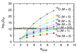
Figure 5: $M$-scheme dimensions as functions of basis-space size, $N_{shell}$.

Besides the $N_{max}$ truncation of the model space in the ab initio shell models, there is the FCI method to give the exact solutions in the fixed model space. Different from the $N_{max}$ truncation in the NCSM and NCFC methods, the FCI truncates the model space by the single-particle states, so-called $N_{shell}$ or $e_{max}(\equiv N_{shell}-1)$. As shown in Fig. 5, the explosion of the dimensionality prohibits the full ab initio solutions of the FCI (and also the NCSM) beyond the lower p-shell region. Similar to the attempts of the IT-NCSM and SA-NCSM, the MCSM is one of the promising candidates to go beyond the FCI method [59, 46]. Note that there is a similar approach to the no-core MCSM referred to as the Hybrid Multi-Determinant method [60]. In the following subsection we will show some recent investigations by the ab initio no-core MCSM.

3.2 Benchmarks of the MCSM to the ab initio no-core FCI

As an exploratory work of the original MCSM has been applied to the no-core calculations for the structure and spectroscopy of the beryllium isotopes [61]. In Ref. [61] the low-lying excited states of ¹⁰Be and ¹²Be are investigated. The excitation energies of the first and second $2^{+}$ states and the B(E2; 2${}^{+}_{1}\rightarrow$ 0${}^{+}_{g.s.}$) for ¹⁰Be with a treatment of spurious center-of-mass motion show good agreement with experimental data. The deformation properties of the $2^{+}_{1}$ and $2^{+}_{2}$ states for ¹⁰Be and of the $2^{+}_{1}$ state for ¹²Be are studied in terms of electric quadrupole moments, E2 transitions and the single-particle occupations. The triaxial deformation of ¹⁰Be is also discussed in terms of the B(E2; 2${}^{+}_{2}\rightarrow$ 2${}^{+}_{1}$) value. This work motivates a further extension of the MCSM application to the ab initio FCI calculations [59]. Currently, the availability of the MCSM for the no-core calculations has been tested extensively in light nuclei [46].

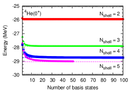
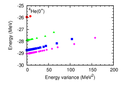
Figure 6: ⁴He ground-state energies as functions of number of basis states (left) and energy variance (right). The red, green, blue and purple solid symbols (horizontal dashed lines in the left figure and open symbols at the zero energy variance in the right figure) are the MCSM (FCI) results in $N_{shell}=2$, $3$, $4$ and $5$, respectively. The harmonic oscillator energies are taken at optimal values for each state and model space. The Coulomb interaction and the spurious center-of-mass motion effect are not considered. Isospin symmetry is assumed.

Figure 7: Comparisons of the energies between the MCSM and FCI along with the fully converged NCFC results where available [46]. The MCSM (FCI) results are shown as the solid (dashed) lines that nearly coincide where both are available. The extrapolated MCSM results are illustrated by bands. From top to bottom, the truncation of the model space is $N_{shell}=2$ (red), $3$ (green), $4$ (blue) and $5$ (purple). Note that the MCSM results are extrapolated by the energy variance with the second-order polynomials [17]. Also note that all of the results of ¹⁰B and ¹²C at $N_{shell}=4$ were obtained only with MCSM.

As a typical example, the behavior of the ground-state energies of ⁴He ($0^{+}$) with respect to the number of basis states and to the energy variance in $N_{shell}=2-5$ are shown in Fig. 6. Figure 7 illustrates the comparisons of the energies for each state and model space between the MCSM and FCI methods. The FCI gives the exact energies in the fixed size of the mode space, while the MCSM gives approximated ones. Thus the comparisons between them show how well the MCSM works in no-core calculations. For this benchmark comparison, the JISP16 two-nucleon interaction is adopted and the Coulomb force is turned off. Isospin symmetry is assumed. The energies are evaluated for the optimal harmonic oscillator frequencies where the calculated energies are minimized for each state and model space. Here the contributions from the spurious center-of-mass motion are ignored for simplicity. In Fig. 7, the comparisons are made for the states; ⁴He($0^{+}$), ⁶He($0^{+}$), ⁶Li($1^{+}$), ⁷Li($1/2^{-}$, $3/2^{-}$), ⁸Be($0^{+}$), ¹⁰B($1^{+}$, $3^{+}$) and ¹²C($0^{+}$). The model space ranges from $N_{shell}=2$ through $5$ for $A\leq 6$ ($4$ for $A\geq 7$). Note that the energies of ¹⁰B($1^{+}$, $3^{+}$) and ¹²C($0^{+}$) in $N_{shell}=4$ are available only from the MCSM results. The $M$-scheme dimensions for these states ($1.82\times 10^{10}$ for $M=1$ and $1.52\times 10^{10}$ for $M=3$ in ¹⁰B and $5.87\times 10^{11}$ for $M=0$ in ¹²C) are already marginal or exceed the current limitation in the FCI approach. The number of basis states are taken up to $100$ in $N_{shell}=2-4$ and $50$ in $N_{shell}=5$. In Fig. 7, the solid (dashed) lines indicate the MCSM (FCI) results. The shaded regions express the extrapolations in the MCSM, and the lower bound of the shaded region corresponds to the extrapolated energy. Furthermore, we also plot the NCFC results for the states of $4\leq A\leq 8$ as the fully converged energies in the infinite model space. As seen in Fig. 7, the energies are consistent with each other where the FCI results are available to within $\sim 100$ keV ($\sim 500$ keV) at most of the MCSM results with(out) the energy-variance extrapolation in the MCSM. The other observables besides the energies also give reasonable agreements between the MCSM and FCI results. The detailed comparisons among the MCSM, FCI and NCFC methods can be found in Ref. Abe:2012wp.

By exploiting the recent development in the computation of the Hamiltonian matrix elements between non-orthogonal Slater determinants [62] and the technique of energy-variance extrapolation [17], the observables give good agreement between the MCSM and FCI results in the $p$-shell nuclei. From the benchmark comparison, the no-core MCSM is now verified in the application to the ab initio no-core calculations for light nuclei. Moreover the application of the no-core MCSM to heavier nuclei is expected in the near future.

3.3 Analysis of intrinsic state

While ab initio approaches have been studied intensively in light nuclei, it is relatively difficult to study the cluster structure in an ab initio way. Among these approaches, the Green’s Function Monte Carlo first provided the two-$\alpha$ structure of the ⁸Be ground state illustratively[64]. This study has shown the possibility that the cluster structure can appear in ⁸Be, without assuming any cluster structure in advance. Generalizing this result, it may be possible to treat cluster structure from a pure single particle picture. In this subsection, we show how to visualize the cluster state in the no-core MCSM calculation and by analyzing the calculations we discuss the appearance of $\alpha$ cluster structure. It is also suited to clarify the relation between the shell-model and cluster pictures [65] from the shell-model point of view. This view point has not been investigated very well yet. Recently, the density profile in the lithium isotopes has been investigated by the NCFC [66]. The method has shown how to calculate the translationally-invariant density. In Li isotopes, the shape distortion and cluster-like structure has been found. Thus, the study of cluster structure has become a realistic subject by using the shell-model calculation.

To extract the cluster structure from the no-core MCSM, we define the intrinsic state to visualize the cluster shape in the intrinsic framework which is extracted from the angular-momentum-projected wave function. The wave function of the no-core MCSM, which is defined in Eq.(5), is represented as an angular-momentum projection of a linear combination of basis states such as

$$|\Psi\rangle=P^{I}|\Phi\rangle\ \ \ \ \ |\Phi\rangle=\sum_{n}f_{n}|\phi_{n}\rangle,$$ (8)

where the total $I$ is assumed to be zero and $K$-quantum number and parity projections are omitted for simplicity. This linear combination of the unprojected basis states, $|\Phi\rangle$, cannot be considered as an intrinsic state because the principal axis of a basis state, $|\phi_{i}\rangle$, is not in the same direction as that of another basis state. Therefore we rotate each basis state so that it has a diagonalized quadrupole-moment; $Q_{zz}>Q_{yy}>Q_{xx}$ and $Q_{ij}=0,(i\neq j)$, respectively, following the concept of Ref. yoshida:2000wp. As a result, these rotated basis states have a large overlap with each other and make a distinct principal axis toward the $z$-axis. The intrinsic wave function $|\Phi^{{\rm intr}}\rangle$ is defined as

$$|\Phi^{{\rm intr}}\rangle \equiv \sum_{n}f_{n}R(\Omega_{n})|\phi_{n}\rangle=\sum_{n}f_{n}|\phi^{R}_{n}\rangle,$$ (9)

where the $R(\Omega_{n})$ is a rotation operator with Euler’s angle $\Omega_{n}$. The $\Omega_{n}$ is determined so that the transformed basis state $|\phi_{n}^{R}\rangle=R(\Omega_{n})|\phi_{n}\rangle$ has the diagonalized quadrupole-moment. The transformed coefficient $D^{R}_{n}$ (by $R(\Omega_{n})$) is derived by the relation in Ref. ppnp_mcsm. This state exactly has the same energy after the angular momentum projection. We calculate the one-body density of the intrinsic state such as

$$\rho^{{\rm intr}}(r) = \langle\Phi^{{\rm intr}}|\sum_{i}\delta(r-r_{i})|\Phi^{{\rm intr}}\rangle,$$ (10)

where $r_{i}$ denotes the position of the $i$-th nucleon.

As an illustrative example, we show the ⁸Be density in $N_{shell}=4$ and $\hbar\omega=20$ MeV with the JISP16 interaction for $J=0^{+}$ states. The Coulomb interaction and the contamination of spurious center-of-mass motion are neglected for simplicity. We show the proton density (a half of the total density) of the $|\Phi\rangle$ and the intrinsic-state density, $\rho^{{\rm intr}}$, in Fig. 8.

The number of basis states is $N_{b}=1,10$ and $100$ for the lower, middle and upper rows, respectively. The energy is almost converged at $N_{b}=100$. Each density distribution is shown along the $yz$ planes at $x=0$ fm and at $x=1$ fm.

Figure 8: ⁸Be proton density for $|\Phi\rangle$ (left panels) and intrinsic (right panels) states for various $N_{b}$ and sliced along the $yz$ plane. The number of basis states is $N_{b}=1,10$ and $100$ for the lower, middle and upper figures, respectively. The slice along the $yz$ plane is the $x=0$ fm plane (left) or $x=1$ fm plane (right) for each panel. The size of each box is 8 fm $\times$ 8 fm.

As shown in the $N_{b}=1$ results, clear deformation and the neck structure to be called a dumbbell shape appear. We can see that as the number of basis states, $N_{b}$, increases the density of $|\Phi\rangle$ are much vague and becomes ordinary prolate rather than dumbbell-like because of the mixture of different directions of principal axes of the basis states. On the other hand, the intrinsic density has clearer dumbbell-like structure for each $N_{b}$. In addition, the density distribution of the intrinsic state is almost unchanged with respect to $N_{b}$. This result indicates the appearance of cluster structure in the no-core MCSM. We also check how the cluster shape differs between $N_{shell}=3$ and $N_{shell}=4$. We find that the neck of dumbbell shape is more enhanced in $N_{shell}=4$ than in $N_{shell}=3$. Since the weights of distribution for both sides of the principal axis are almost the same, this cluster can be considered as two $\alpha$ clusters. The stability of the $\alpha$ cluster is confirmed with respect to $N_{b}$ and $N_{shell}$. This result is consistent with the result of the Green’s Function Monte Carlo [64]. With the use of this method to draw the density, we can study the appearance of cluster structure directly not only for $N=Z$ nuclei but also for the neutron-rich nuclei in the ab initio approach. The study of exotic structure including unstable nuclei in the $p$-shell region is in progress.

4 Application to neutron-rich Cr and Ni isotopes

In this section, we discuss the application of the MCSM to the large-scale shell-model calculations about neutron-rich Cr and Ni isotopes as examples. We take a model space as the $pfg_{9}d_{5}$ shell, which consists of the $0f1p$ shell, the $0g_{9/2}$ orbit, and the $1d_{5/2}$ orbit. By using such a sufficiently large model space, we aim at a unified description of medium-heavy nuclei and at studying the shell evolution [18, 19, 20, 21] and the magicity of $N=28,40,50$ microscopically.

4.1 Ni isotopes and magicity of $N=28,40,50$.

The nuclear shell structure evolves in neutron-rich nuclei and the magic numbers of unstable nuclei are different from those of stable nuclei. The large excitation energy of the $2^{+}$ yrast state and the small $B(E2;0^{+}\rightarrow 2^{+})$ value in ⁶⁸Ni ($Z=28$, $N=40$) might indicate that ⁶⁸Ni is a double-magic nucleus, although $N=40$ is a magic number of the harmonic oscillator, not a magic number of the nuclear shell model. On the other hand, the small excitation energies of the $2^{+}$ yrast state and the large $B(E2;0^{+}\rightarrow 2^{+})$ values in Cr ($Z=24$) isotopes of $N\sim 40$ suggest rather strong deformation. This change of the $N=40$ gap has been studied theoretically [67]. ⁷⁸Ni, which has $Z=28$ and $N=50$ doubly magic numbers, has also been investigated to discuss its magicity and the size of $N=50$ gap [74].

In the $sd$-shell and the light $pf$-shell regions, we can describe properties of stable nuclei in relatively small model spaces. However, we sometimes need a large model space to describe the properties of neutron-rich nuclei. In order to discuss neutron-rich Ni isotopes up to $N=50$, it is essential to include the effects of excitation across the $Z=28$ and $N=50$ gaps by adopting the $pfg_{9}d_{5}$ model space. Concerning this model space, M. Honma et al. proposed the A3DA effective interaction [68] which consists of the GXPF1A [69], JUN45 [41], and $G$-matrix effective interactions with phenomenological modifications. It has succeeded in describing the neutron-rich Cr and Ni isotopes under a severe truncation of the model space utilizing the few-dimensional basis approximation [26]. In this work, we use the new version of the MCSM method, which enables us to precisely evaluate the exact shell-model energy without any truncation and discuss the effective interaction.

4.2 Effective interaction for $pfg_{9}d_{5}$ shell

In this section, we discuss the A3DA effective interaction [68] and its improvement. The two-body matrix elements (TBMEs) of the A3DA interaction consist of three parts. The TBMEs of the $pf$ shell are those of the GXPF1A interaction [69], which is successful for describing spectroscopic properties of light $pf$-shell nuclei. The TBMEs of the $f_{5}pg_{9}$ shell related to the $0g_{9/2}$ orbit are those of the JUN45 interaction [41]. The GXPF1A and JUN45 interactions were determined by combining microscopically derived interactions ($G$ matrix) with a minor empirical fit so as to reproduce experimental data. The other TBMEs are from the $G$-matrix effective interaction[70, 71], which is calculated from the chiral N3LO interaction[48]. The Coulomb interaction is not included and the isospin symmetry is conserved. The $G$ matrix is calculated for the $pfsdg$ shell with ⁴⁰Ca as an inert core and the core-polarization correction is included perturbatively. The single-particle energies and the monopole interaction are adjusted to reproduce the GXPF1A and JUN45 predictions for the $pf$ shell and $g_{9/2}$ orbits, and the Woods-Saxon single-particle energies of stable semi-magic nuclei for the other part.

The original A3DA interaction failed to describe some nuclei around $N\sim 40$. We modify mainly single-particle energies and monopole components related to the $0g_{9/2}$ orbit by comparing the results of the calculations with the experiments. These calculations are far beyond the current limitation of the conventional diagonalization method, and the MCSM method enables us to perform this comparison.

4.3 MCSM results of the neutron-rich Cr and Ni isotopes

We performed systematic calculations of the $0^{+}$ and $2^{+}$ yrast states of neutron-rich Cr and Ni even-even isotopes using the MCSM method and the modified A3DA interaction. We took 50 basis states for the MCSM with the refinement procedure, which is discussed in Sect.2.2. The energies were extrapolated by the energy-variance extrapolation method and the other values were not. The effective charges are taken as $(e_{p},e_{n})=(1.5,0.5)e$.

Figure 9: The excitation energies of $2^{+}_{1}$ states (left) and $B(E2;0^{+}_{1}\rightarrow 2^{+}_{1})$ values (right) obtained by the MCSM for Cr isotopes. Experimental data are taken from Refs.[72, 73].

Figure 9 shows the $2^{+}$ excitation energies and the $B(E2)$ transition probabilities of neutron-rich Cr isotopes. The MCSM results well reproduce the experimental values while the modest overestimation remains. The Cr isotopes do not show any feature of $N=40$ magicity, while the characteristics of $N=28$ magicity can be seen, namely, a sudden increase of excitation energy and slight decrease of the $B(E2)$ value. On the neutron-rich side, the excitation energy decreases and the $B(E2)$ value increases gradually as the neutron number increases, which implies gradual enhancement of the quadrupole deformation.

Figure 10: $2^{+}$ excitation energies for Ni isotopes. Experimental data are taken from Ref.nudat.

Figure 11: $B(E2;0^{+}\rightarrow 2^{+})$ values for Ni isotopes. Experimental data are taken from Ref.BE2.

Figure 12: Occupation numbers of the neutron $g_{9/2}$ orbit for Ni isotopes.

Figure 13: Two-neutron separation energies $S_{2n}$ for Ni isotopes. Experimental data are taken from Ref.nudat.

Figure 14: Total energy surface of $0^{+}_{1}$ (left) and $0^{+}_{2}$ (right) states of ⁶⁸Ni. The positions of red circles represent quadrupole deformations of the MCSM basis states before projection. The areas of those circles represent the overlap probabilities of the basis states and the resulting wave function.

Figure 11 shows $2^{+}$ excitation energies of Ni ($Z=28$) even-even isotopes from ⁵⁶Ni to ⁷⁸Ni. The large $2^{+}$ excitation energy of ⁵⁶Ni ($N=28$) indicates $Z=28$, $N=28$ double magicity. The large value of the calculated $2^{+}$ excitation energy of ⁷⁸Ni ($N=50$) suggests $Z=28$, $N=50$ double magicity. The large $2^{+}$ excitation energy of ⁶⁸Ni ($N=40$) indicates $N=40$ magicity. The calculated values reproduce the experimental values well.

Figure 11 shows $B(E2;0^{+}\rightarrow 2^{+})$ for neutron-rich Ni isotopes. The small value of $B(E2;0^{+}\rightarrow 2^{+})$ at $N=40$ indicates $N=40$ magicity. Neither the theoretical nor experimental value of $B(E2;0^{+}\rightarrow 2^{+})$ at $N=28$ is small unlike that at the $N=40$, and the theoretical $B(E2;0^{+}\rightarrow 2^{+})$ value at $N=50$ becomes large in comparison with those of neighboring nuclei. It suggests that at $N=28,50$ magicity is broken to some extent for ^56,78Ni, respectively. Figure 13 shows the occupation number of the neutron $g_{9/2}$ orbit. The occupation numbers of $0^{+}$ and $2^{+}$ states are very close for Ni isotopes besides ^68,78Ni ($N=40,50$). The occupation numbers of the $2^{+}$ states of ^68,78Ni show a breakdown of the closed-shell structure. Figure 13 shows two-neutron separation energies. The calculated values of neutron-rich nuclei are smaller than experimental values. This means that the binding energies of neutron-rich nuclei are underestimated. The values of $S_{2n}$ increase slightly by considering the Coulomb energy, but calculated values are still smaller than experimental values.

Figure 14 shows the total energy surface of ⁶⁸Ni provided by the $Q$-constrained Hartree-Fock calculation [77]. There are three minimum points for ⁶⁸Ni. Figure 14 also shows quadrupole deformations of the MCSM wave functions of the $0^{+}_{1}$ and $0^{+}_{2}$ states. The scattered circles correspond to the basis states in the MCSM wave function. The position of the circle indicates the quadrupole deformation of the basis state before projection. The area of the circle is proportional to the overlap probability of the projected basis and the resulting wave function. It is quite clear that the $0^{+}_{1}$ state of ⁶⁸Ni corresponds to a spherical shape and the $0^{+}_{2}$ state corresponds to an oblate shape. Spherical and oblate components are mixed to some extent, but the components of the prolate minimum hardly mix.

Figure 15: ESPEs of the neutron orbits for Ni ($Z=28$) isotopes.

Figure 16: ESPEs of the neutron orbits for $N=40$ isotones.

Furthermore, we consider the magicity and the energy gaps for Ni isotopes by using the effective single particle energies (ESPEs) [75]. Figure 16 shows ESPEs of the neutron orbits for Ni isotopes. The $f_{7/2}$-$p_{3/2}$ gap at $N=28$ is $7.1$ MeV and gives the magicity to ⁵⁶Ni. The $g_{9/2}$-$d_{5/2}$ gap at $N=50$ is $4.2$ MeV and gives the magicity to ⁷⁸Ni. This is partly due to the additional lowering of the $g_{9/2}$ orbit caused by pairing correlation between two neutrons in the $g_{9/2}$ orbit, and also due to the effect of the two-neutron repulsive monopole interaction originating in the three-nucleon force like in exotic oxygen isotopes [21]. The $p_{1/2}$-$g_{9/2}$ gap at $N=40$ is $2.6$ MeV, which is smaller than the $N=28,50$ gaps. Figure 16 shows the ESPEs of the neutron orbits for $N=40$ isotones. As the proton number of $f_{7/2}$ increases from $Z=20$ to $Z=28$, the ESPE of $f_{5/2}$ lowers and the $N=40$ gap becomes larger. Because of this evolution of the $N=40$ gap, the properties of $N\sim 40$ nuclei depend on the proton number.

Figure 17: ESPEs of the proton orbits for Ni isotopes (left) and for $N=40$ isotones (right).

In Fig. 17, the ESPEs of the proton orbits for Ni isotopes and for $N=40$ isotones are shown. In the former, rapid lowering of the $f_{5/2}$ orbit from $N=40$ to 50 is clearly seen as suggested in [19, 20], while narrowing of $Z=28$ gap is also visible there. Such changes are responsible partly for the origins of the structure evolution in these Ni isotopes.

5 Summary and future perspectives

We have developed a new generation of the MCSM by introducing the conjugate gradient method and the energy-variance extrapolation, which enhance the applicability of the MCSM greatly. We have two major scopes of this framework: ab initio shell-model calculations and conventional shell-model calculations assuming an inert core. In the former, we have compared the MCSM results with the exact FCI calculations to demonstrate the validity of the MCSM framework and its feasibility beyond the limit of the FCI in Sect.3. In addition, we have proposed a novel method to discuss the intrinsic structure and demonstrated that the cluster structure appears in shell-model-type calculations based on the harmonic-oscillator-basis wave function. In the latter, we discussed in Sect.4 that the MCSM enables us to perform shell-model calculations of neutron-rich Cr and Ni isotopes in the $pfg_{9}d_{5}$ model space in which the isospin symmetry is conserved. We proposed a “modified A3DA” interaction which reproduces the low-lying spectra of neutron-rich Cr and Ni isotopes and guides us towards a unified description including ⁵⁶Ni, ⁶⁸Ni and ⁷⁸Ni, with magic numbers 28, 40, 50, respectively. The prediction of ⁷⁸Ni is especially interesting to see the evolution of shell structure. On the other hand, Cr isotopes do not show any feature of $N=40$ magicity and the collectivity enhances as the neutron number increases. The MCSM and newly proposed effective interaction are expected to provide us with a unified description of $pf$-shell nuclei.

The current status of the computer-code development was also reported in Sect.2.5. At the present stage, we have obtained good parallel scalability of our code up to $10^{5}$ CPU cores via early access to the K computer at RIKEN AICS[76] as measured by the benchmark test. However, such good scalability is not always obtained and further development is in progress. This activity is promoted strongly as a part of the activities of HPCI Strategic Programs for Innovative Research (SPIRE) Field 5 “The origin of matter and the universe”.

By utilizing both the developed code and the K computer, we promote further large-scale shell-model calculations as a part of the SPIRE activities. We plan to perform systematic study with ab initio calculations of light nuclei in $N_{shell}=5$ and some states in $N_{shell}=6$. Concerning the medium-heavy nuclei, because it is difficult to cover whole region of the nuclear chart, we will choose some interesting nuclides as subjects of our investigation, and will perform shell-model calculations of these nuclides with the two-major-shell model space. For example, the shell-model calculations of ¹³⁰Te, ¹²⁸Te, and ¹⁵⁰Nd are extremely interesting to study double beta decay and the nuclear matrix element of neutrinoless decay. We also continue to study the systematic calculations of neutron-rich $pf$-shell nuclei to discuss the shell-evolution phenomenon.

Appendix A Numeration with projected Slater determinants

In this appendix, we show some equations which are needed to perform the calculation discussed in Sect.2.

At the beginning, we define a deformed Slater determinant,

$$|\phi\rangle=\prod_{k=1}^{N_{\rm f}}\left(\sum_{l=1}^{N_{\rm sp}}D_{lk}c^{\dagger}_{l}\right)|-\rangle,$$ (11)

which is parametrized by the complex $N_{\rm sp}\times N_{\rm f}$ matrix $D$ with the normalization condition $D^{\dagger}D=1$. $N_{\rm f}$ and $N_{\rm sp}$ are the numbers of fermions and single-particle states, respectively. The $|-\rangle$ denotes an inert core in the conventional shell-model calculations or the vacuum in ab initio shell-model calculations. Because we do not mix the proton and neutron space in practical calculations, the wave function is written as a product of proton and neutron Slater determinants, namely, $|\phi\rangle=|\phi_{\rm proton}\rangle\otimes|\phi_{\rm neutron}\rangle$. For simplicity, we do not write this isospin degree of freedom explicitly. One can easily reproduce the equations representing the explicit proton-neutron degree of freedom by taking $D$ of the proton-neutron sector as zero such as

$$D=\left(\begin{array}[]{cc}D^{\pi}&0\\ 0&D^{\nu}\end{array}\right)$$ (12)

where $D^{\pi}$ and $D^{\nu}$ represent Slater determinants of protons and neutrons, respectively.

The angular-momentum, parity projector $P^{I\pi}_{MK}$ in Eq.(6) is performed by discretizing the integral concerning the Euler angles such as

$$P^{I\pi}_{MK}=\sum_{\lambda}W^{I\pi(\lambda)}_{MK}R^{(\lambda)}$$ (13)

where the $\lambda$ denotes an index of mesh point of the discretization (here, a set of Euler’s angle $\Omega=(\alpha,\beta,\gamma)$ and parity variable $\pi^{\lambda}=\pm 1$). In this paper, the parity projection is described by the summation of 2 mesh points such as $P^{\pi}=\frac{1+\pi\Pi}{2}=\sum_{\lambda=1}^{2}\pi^{(\lambda)}\Pi^{(\lambda)}$ with $\pi^{(1)}=\frac{1}{2}$, $\pi^{(2)}=\frac{\pi}{2}$, $\Pi^{(1)}=1$, and $\Pi^{(2)}=\Pi$ with $\Pi$ being the parity-conversion operator. $W^{(\lambda)}$ is a weight of the mesh point $\lambda$, and $R^{(\lambda)}$ is a product of the rotation and parity-conversion operators such as

$$W^{I\pi(\lambda)}_{MK} = \frac{2I+1}{8\pi^{2}}D^{I*}_{MK}(\alpha_{\lambda},\beta_{\lambda},\gamma_{\lambda})\pi^{(\lambda)},$$

$$R^{(\lambda)} = e^{i\alpha_{\lambda}J_{z}}e^{i\beta_{\lambda}J_{y}}e^{i\gamma_{\lambda}J_{z}}\Pi^{(\lambda)}.$$ (14)

Note that the operator $R^{\lambda}$ does not change the form of a Slater determinant, i.e.,

$$|\phi^{(\lambda)}_{n}\rangle=R^{(\lambda)}|\phi_{n}\rangle,$$ (15)

where a matrix $D^{n(\lambda)}$ represents the single Slater determinant $|\phi^{(\lambda)}_{n}\rangle$, thanks to the Baker-Hausdorff’s theorem [12].

The norm matrix and hamiltonian matrix spanned by $N$ Slater determinants are written as

$${\cal N}_{mM,nK} = \langle\phi_{m}|P^{I\pi}_{MK}|\phi_{n}\rangle$$ (16)

$${\cal H}_{mM,nK} = \langle\phi_{m}|HP^{I\pi}_{MK}|\phi_{n}\rangle.$$ (17)

The coefficient, $f_{nK}$ in Eq.(5), is determined by solving the generalized eigenvalue problem

$$\sum_{nK}{\cal H}_{mM,nK}f_{nK}={\cal E}\sum_{nK}{\cal N}_{mM,nK}f_{nK},$$ (18)

and the normalization condition $\langle\Psi|\Psi\rangle=1$. The lowest eigenvalue of ${\cal E}$ is taken as $E_{N}$ if you would like to obtain the yrast state.

By combining Eqs. (13) and (16), the norm matrix is calculated as

$${\cal N}_{mM,nK}=\sum_{\lambda}W^{I\pi(\lambda)}_{MK}\langle\phi_{m}|R^{(\lambda)}|\phi_{n}\rangle=\sum_{\lambda}W^{I\pi(\lambda)}_{MK}\langle\phi_{m}|\phi_{n}^{(\lambda)}\rangle,$$ (19)

with

$$\langle\phi_{m}|\phi_{n}^{(\lambda)}\rangle={\rm det}\left(D^{m\dagger}D^{n(\lambda)}\right).$$ (20)

In the same way, the hamiltonian matrix is obtained as

$${\cal H}_{mM,nK} = \sum_{\lambda}W^{I\pi(\lambda)}_{MK}\langle\phi_{m}|HR^{(\lambda)}|\phi_{n}\rangle$$

$$= \sum_{\lambda}W^{I\pi(\lambda)}_{MK}\langle\phi_{m}|\phi_{n}^{(\lambda)}\rangle{\rm Tr}\left(\rho^{(\lambda)}(t+\frac{1}{2}\Gamma^{(\lambda)})\right).$$

where the generalized density matrix, $\rho^{(\lambda)}$, and the self-consistent field, $\Gamma^{(\lambda)}$, [77] are defined as

$$\rho^{(\lambda)}_{ij}=\frac{\langle\phi_{m}|c^{\dagger}_{j}c_{i}|\phi^{(\lambda)}_{n}\rangle}{\langle\phi_{m}|\phi_{n}^{(\lambda)}\rangle}=(D^{n(\lambda)}(D^{m\dagger}D^{n(\lambda)})^{-1}D^{m\dagger})_{ij}$$ (22)

$$\Gamma^{(\lambda)}_{ik} = \sum_{jl}\overline{v}_{ijkl}\rho^{(\lambda)}_{lj}$$ (23)

with $\overline{v}_{ijkl}=v_{ijkl}-v_{ijlk}$. The trivial summations and their indices for the matrix products are omitted for readability. The indices $m,n$ of $\rho^{(\lambda)}$ and $\Gamma^{(\lambda)}$ are also omitted.

The most-time-consuming part is the calculation of the $\Gamma^{(\lambda)}_{ik}$, which can be rewritten following the idea of Ref.[42],

$$\Gamma^{(\lambda)}_{a} = \sum_{b}\overline{v}_{ab}\rho^{(\lambda)}_{b}$$ (24)

where $a=(i,k)$, and $b=(j,l)$. Because $\overline{v}_{ab}$ is a block-antidiagonal form owing to the symmetry of the Hamiltonian, Eq.(24) is calculated as the products of the dense block matrices and the dense matrices in terms of the indices $a,b,\lambda$ efficiently avoiding trivial zero matrix elements of $v_{ab}$. This method is referred to as the matrix-matrix method in Ref.mcsm_tuning. This matrix-matrix method enables us to use a CPU utilizing the BLAS level 3 library quite efficiently, and the performance reaches $70\sim 80\%$ of the theoretical peak performance [42].

This efficient computation of $\Gamma^{(\lambda)}$ is useful also for the evaluation of the energy gradient, which is essential for the conjugate gradient method. The energy gradient of the Slater-determinant coefficients is written as

$$\frac{\partial E_{N}}{\partial D^{m*}} = (1-D^{m}D^{m\dagger})\sum_{M,n,K,\lambda}f_{mM}^{*}f_{nK}W^{I\pi(\lambda)}_{MK}\langle\phi_{m}|\phi^{(\lambda)}_{n}\rangle$$

$$\times\left((1-\rho^{(\lambda)})(t+\Gamma^{(\lambda)})+\left({\rm Tr}\bigl{(}(t+\frac{1}{2}\Gamma^{(\lambda)}\bigr{)}\rho^{(\lambda)}\bigr{)}-E_{N}\right)\right)\rho^{(\lambda)}D^{m}.$$

To evaluate the energy variance $\langle\Delta H^{2}\rangle_{N}=\langle H^{2}\rangle_{N}-E_{N}^{2}$, the expectation value of the $H^{2}$ with the wave function in Eq.(5) is written as

$$\langle\Psi_{N}|H^{2}|\Psi_{N}\rangle = \sum_{m,M,n,K,\lambda}f_{mM}^{*}f_{nK}W^{I\pi(\lambda)}_{MK}\langle\phi_{m}|H^{2}|\phi_{n}^{(\lambda)}\rangle.$$ (26)

From Ref.mcsm_extrap, the matrix element of the Hamiltonian squared is computed such as

$$\frac{\langle\phi_{m}|H^{2}|\phi^{(\lambda)}_{n}\rangle}{\langle\phi_{m}|\phi^{(\lambda)}_{n}\rangle} = \sum_{i<j,k<l,\alpha<\beta,\gamma<\delta}v_{ijkl}\Theta^{(\lambda)}_{kl\alpha\beta}v_{\alpha\beta\gamma\delta}\Lambda^{(\lambda)}_{\gamma\delta ij}$$

$$+{\rm Tr}((t+\Gamma^{(\lambda)})(1-\rho^{(\lambda)})(t+\Gamma^{(\lambda)})\rho^{(\lambda)})+\left({\rm Tr}(\rho^{(\lambda)}(t+\frac{1}{2}\Gamma^{(\lambda)}))\right)^{2}$$

$$\Lambda^{(\lambda)}_{ijkl} = \rho^{(\lambda)}_{ik}\rho^{(\lambda)}_{jl}-\rho^{(\lambda)}_{il}\rho^{(\lambda)}_{jk}$$ (28)

$$\Theta^{(\lambda)}_{ijkl} = (1-\rho^{(\lambda)})_{ik}(1-\rho^{(\lambda)})_{jl}-(1-\rho^{(\lambda)})_{il}(1-\rho^{(\lambda)})_{jk}.$$ (29)

The most-time-consuming part in the evaluation of the energy variance is to calculate the first term of the right-hand side of Eq.(A). By substituting $(i,j),(k,l),(\alpha,\beta)$, and $(\gamma,\delta)$ by $a,b,c$, and $d$, respectively, this term is efficiently calculated as the products of the matrices, namely, $\sum_{abcd}v_{ab}\Theta_{bc}v_{cd}\Lambda_{da}$. Note that the $v_{ab}$ has a block-diagonal form, which again enables us to use the BLAS level 3 library, avoiding trivial zero matrix elements.

Another formulation to compute the expectation values in projected Slater determinants can be found in Refs.[29, 78], in which the two-body interaction is decomposed into a sum of the squares of the one-body operators.

References

- [1] H. Kamada et al., \PRC64,2001,044001.
- [2] M. G. Mayer, \PR75,1949,1969; O. Hazel, J. H. D. Jensen, and H. E. Suess, \PR75,1949,1766.
- [3] B. A. Brown and B. H. Wildenthal, Ann. Rev. Nucl. Part. Sci. 38 (1988), 29.
- [4] B. A. Brown and W. A. Richter, \PRC74,2006,034315.
- [5] A. Poves, J. Sánchez-Solano, E. Caurier, and F. Nowacki, \NPA694,2001,157.
- [6] M. Honma, T. Otsuka, B. A. Brown, and T. Mizusaki, \PRC65,2002,061301(R); \PRC69,2004,034335.
- [7] P. Navrátil, J. P. Vary, and B. R. Barrett, Phys. Rev. Lett. 84 (2000), 5728; Phys. Rev. C 62 (2000), 054311; S. Quaglioni and P. Navrátil, Phys. Rev. Lett. 101 (2008), 092501; Phys. Rev. C 79 (2009), 044606.
- [8] SciDAC Review, Issue 6 (2007), pp. 42-51.
- [9] M. Honma, T. Mizusaki, and T. Otsuka, \PRL77,1996,3315.
- [10] M. Honma, T. Mizusaki, and T. Otsuka, Phys. Rev. Lett. 75 (1995), 1284.
- [11] S. E. Koonin, D. J. Dean, and K. Langanke, Phys. Rep. 278 (1997), 1.
- [12] T. Otsuka, M. Honma, T. Mizusaki, N. Shimizu, and Y. Utsuno, Prog. Part. Nucl. Phys. 47 (2001), 319.
- [13] N. Shimizu, T. Otsuka, T. Mizusaki, and M. Honma, \PRL86,2001,1171.
- [14] K. W. Schmid, Prog. Part. Nucl. Phys. 52 (2004), 565.
- [15] T. Otsuka, M. Honma, and T. Mizusaki, \PRL81,1998,1588.
- [16] N. Shimizu, Y. Utsuno, T. Abe, and T. Otsuka, RIKEN Accel. Prog. Rep. 43 (2010), 46.
- [17] N. Shimizu, Y. Utsuno, T. Mizusaki, T. Otsuka, T. Abe, and M. Honma, Phys. Rev. C 82 (2010), 061305(R).
- [18] T. Otsuka, R. Fujimoto, Y. Utsuno, B. A. Brown, M. Honma, and T. Mizusaki, Phys. Rev. Lett. 87 (2001), 082502.
- [19] T. Otsuka, T. Suzuki, R. Fujimoto, H. Grawe, and Y. Akaishi, Phys. Rev. Lett. 95 (2005), 232502.
- [20] T. Otsuka, T. Suzuki, M. Honma, Y. Utsuno, N. Tsunoda, K. Tsukiyama, and M. H.-Jensen, Phys. Rev. Lett. 104, (2010), 012501.
- [21] T. Otsuka, T. Suzuki, J. D. Holt, A. Schwenk, and Y. Akaishi, Phys. Rev. Lett. 105, (2010) 032501.
- [22] B. A. Brown, Prog. Part. Nucl. Phys. 47 (2001), 517.
- [23] N. Shimizu, Y. Utsuno, T. Mizusaki, T. Otsuka, T. Abe and M. Honma, AIP Conf. Proc. 1355 (2011), 138.
- [24] A. M. Shirokov, J. P. Vary, A. I. Mazur and T. A. Weber, Phys. Letts. B 644 (2007), 33; A. M. Shirokov, J. P. Vary, A. I. Mazur, S. A. Zaytsev and T. A. Weber, Phys. Lett. B 621 (2005), 96; subroutines to generate this interaction in the relative-center-of-mass HO basis are available at nuclear.physics.iastate.edu
- [25] D.H. Gloeckner and R.D. Lawson, Phys. Lett. 53B (1974), 313.
- [26] M. Honma, B. A. Brown, T. Mizusaki, and T. Otsuka, Nucl. Phys. A 704, (2002), 134c, M. Honma, T. Otsuka, B.A. Brown and T. Mizusaki, Phys. Rev. C 65 (2002), 061301(R).
- [27] K. W. Schmid, Prog. Part. Nucl. Phys. 52 (2004), 565.
- [28] G. Puddu, Eur. Phys. J. A 34 (2007), 413.
- [29] G. Puddu, J. Phys. G: Nucl. Part. Phys. 32 (2006), 321.
- [30] Numerical Recipes in Fortran 77, the Art of Scientific Computing, 2nd ed., Cambridge University Press: Cambridge, (1992).
- [31] J. L. Egido, J. Lessing, V. Martin, L. M. Robledo, Nucl. Phys. A 594 (1995), 70.
- [32] T. Mizusaki, N. Shimizu, Y. Utsuno, and M. Honma, code MSHELL64, unpublished.
- [33] M. Horoi, A. Volya, and V. Zelevinsky, Phys. Rev. Lett. 82 (1999), 2064; M. Horoi, B. A. Brown, and V. Zelevinsky, Phys. Rev. C 67 (2003), 034303.
- [34] T. Mizusaki and M. Imada, Phys. Rev. C 65 (2002), 064319; ibid. 67 (2003), 041301.
- [35] T. Papenbrock and D. J. Dean, Phys. Rev. C 67 (2003), 051303(R).
- [36] J.J. Shen, Y. M. Zhao, A. Arima, and N. Yoshinaga, Phys. Rev. C 83 (2011), 044322.
- [37] M. Imada and T. Kashima, J. Phys. Soc. Jpn. 69 (2000), 2723.
- [38] W.A. Richter, M.G. van der Merwe, R.E. Julies and B.A. Brown, Nucl. Phys. A523, 325, (1991).
- [39] N. Shimizu, Y. Utsuno, T. Mizusaki, M. Honma, Y. Tsunoda, and T. Otsuka, Phys. Rev. C, 85 (2012), 054301.
- [40] T. Mizusaki, T. Otsuka, Y. Utsuno, M. Honma and T. Sebe, Phys. Rev. C 59 (1999), R1846.
- [41] M. Honma, T. Otsuka, T. Mizusaki, and M. Hjorth-Jensen, Phys. Rev. C 80 (2009), 064323.
- [42] Y. Utsuno, N. Shimizu, T. Otsuka and T. Abe, arXiv:1202.2957 [nucl-th] (2012).
- [43] M. Honma et al., unpublished.
- [44] Intel Math Kernel Library, http://software.intel.com/en-us/articles/intel-mkl/
- [45] T2K Open Supercomputers, http://www.cc.u-tokyo.ac.jp/system/ha8000/
- [46] T. Abe, P. Maris, T. Otsuka, N. Shimizu, Y. Utsuno and J. P. Vary, arXiv:1204.1755 [nucl-th].
- [47] E. Epelbaum, W. Glöckle, and Ulf-G. Meissner, Nucl. Phys. A 637 (1998), 107; 671 (2000), 295.
- [48] D. R. Entem and R. Machleidt, Phys. Rev. C 68 (2003), 041001(R).
- [49] R. B. Wiringa, V. G. J. Stoks and R. Schiavilla, Phys. Rev. C 51 (1995), 38.
- [50] S. C. Pieper, V. R. Pandharipande, R. B. Wiringa, and J. Carlson, Phys. Rev. C 64 (2001), 014001.
- [51] S. C. Pieper, AIP Conf. Proc. 1011 (2008), 143.
- [52] S. C. Pieper, R. B. Wiringa, and J. Carlson, Phys. Rev. C 70 (2004), 054325; K. M. Nollett, S. C. Pieper, R. B. Wiringa, J. Carlson, and G. M. Hale Phys. Rev. Lett. 99 (2007), 022502; S. C. Pieper Proceedings of the International School of Physics ”Enrico Fermi”, Course CLXIX, edited by A. Covello, F. Iachello and R. A. Ricci (Societ Italiana di Fisica, Bologna, 2008) 111. arXiv:0711.1500v1 [nucl-th]; Reprinted in La Rivista del Nuovo Cimento, 31 (2008), 709; and references therein.
- [53] G. Hagen, T. Papenbrock and M. Hjorth-Jensen, Phys. Rev. Lett. 104 (2010), 182501 and references therein.
- [54] S. Okubo, Prog. Theor. Phys. 12 (1954), 603; S. Y. Lee and K. Suzuki, Phys. Lett. B, 91 (1980), 173; K. Suzuki and S. Y. Lee, Prog. Theor. Phys. 64 (1980), 2091; K. Suzuki, R. Okamoto, Prog. Theor. Phys. 70 (1983), 439.
- [55] S. K. Bogner, R. J. Furnstahl and A. Schwenk, Prog. Part. Nucl. Phys. 65 (2010), 94.
- [56] P. Maris, J. P. Vary, P. Navratil, W. E. Ormand, H. Nam and D. J. Dean, Phys. Rev. Lett. 106 (2011), 202502.
- [57] R. Roth, Phys. Rev. C 79 (2009), 064324; R. Roth, S. Binder, K. Vobig, A. Calci, J. Langhammer and P. Navratil, arXiv:1112.0287 [nucl-th].
- [58] T. Dytrych, K. D. Sviratcheva, C. Bahri, J. P. Draayer and J. P. Vary, Phys. Rev. Lett. 98 (2007), 162503; T. Dytrych, K. D. Sviratcheva, C. Bahri, J. P. Draayer and J. P. Vary, J. Phys. G. 35 (2008), 095101; T. Dytrych, K. D. Sviratcheva, J. P. Draayer, C. Bahri and J. P. Vary, J. Phys. G. 35 (2008), 123101.
- [59] T. Abe, P. Maris, T. Otsuka, N. Shimizu, Y. Utsuno, and J. P. Vary, AIP Conf. Proc. 1355 (2011), 173.
- [60] G. Puddu, arXiv:1201.0600 [nucl-th].
- [61] L. Liu, T. Otsuka, N. Shimizu, Y. Utsuno and R. Roth, Phys. Rev. C in press.
- [62] Y. Utsuno, N. Shimizu, T. Otsuka and T. Abe, arXiv:1202.2957 [nucl-th].
- [63] P. Maris, J. P. Vary, A. M. Shirokov, Phys. Rev. C 79 (2009), 014308; P. Maris, A. M. Shirokov and J. P. Vary, Phys. Rev. C 81 (2010), 021301(R); C. Cockrell, J. P. Vary and P. Maris, arXiv:1201.0724.
- [64] R. B. Wiringa, S. C. Pieper, J. Carlson, and V. R. Pandharipande, Phys. Rev. C 62 (2000), 014001.
- [65] N. Itagaki, H. Masui, M. Ito, and S. Aoyama, Phys. Rev. C 71 (2005), 064307.
- [66] C. Cockrell, J. P. Vary and P. Maris, arXiv:1201.0724 [nucl-th].
- [67] S. M. Lenzi, F. Nowacki, A. Poves, and K. Sieja, \PRC82,2010,054301.
- [68] M. Honma et al., unpublished.
- [69] M. Honma, T. Otsuka, B. A. Brown, and T. Mizusaki, Eur. Phys. J. A 25 (2005), s01, 499.
- [70] M. Hjorth-Jensen, T. T. S. Kuo, and E. Osnes, \PR261,1995,125.
- [71] M. Hjorth-Jensen, private communication.
- [72] National Nuclear Data Center, information extracted from the NuDat 2 database, http://www.nndc.bnl.gov/nudat2/
- [73] B. Pritychenko, J. Choquette, M. Horoi, B. Karamy, and B. Singh, arXiv:1102.3365v2.
- [74] M.-G. Porquet, and O. Sorlin, \PRC85,2012,014307
- [75] Y. Utsuno, T. Otsuka, T. Mizusaki, and M. Honma, Phys. Rev. C 60 (1999), 054315.
- [76] K computer, http://www.aics.riken.jp/en/
- [77] P. Ring and P. Schuck, The Nuclear Many-Body Problem, Springer-Verlag, New York, 1980.
- [78] G. Puddu, arXiv:1201.0600 [nucl-th].