DETECTION OF IRON K EMISSION FROM A COMPLETE SAMPLE OF SUBMILLIMETER GALAXIES
Abstract
We present an X-ray stacking analysis of a sample of 38 submillimeter galaxies with discovered at significance in the Lockman Hole North with the MAMBO array. We find a detection in the stacked soft band (0.5–) image, and no significant detection in the hard band (2.0–). We also perform rest-frame spectral stacking based on spectroscopic and photometric redshifts and find a detection of emission with an equivalent width of . The centroid of the emission lies near , indicating a possible contribution from highly ionized Fe XXV or Fe XXVI; there is also a slight indication that the line emission is more spatially extended than the X-ray continuum. This is the first X-ray analysis of a complete, flux-limited sample of SMGs with statistically robust radio counterparts.
1 Introduction
Submillimeter galaxies (SMGs) are distant star-forming systems with tremendous infrared luminosities ( [8–1000). In the (sub)millimeter waveband they are observable out to high redshifts due to the strong negative -correction in the Rayleigh-Jeans regime of their thermal spectrum (see, e.g., Blain et al., 2002). The prevalence of SMGs at (Chapman et al., 2005) in combination with their high rates of dust-obscured star-formation imply that they may be responsible for the production of a significant fraction of all the stellar mass in present-day galaxies. X-ray (Alexander et al., 2003, 2005b) and mid-infrared (Valiante et al., 2007; Menéndez-Delmestre et al., 2007, 2009; Pope et al., 2008) spectroscopy shows that SMGs frequently contain active galactic nuclei (AGN) as well as powerful starbursts. This connection between star formation and accretion at high redshift may help explain the black hole mass-bulge mass relation in present-day galaxies (e.g., Alexander et al., 2005a). However, it remains hard to determine the relative importance of accretion and star formation for the SMG population as a whole because of the challenge of assembling large, statistically unbiased SMG samples.
Studying the X-ray properties of SMGs is difficult for two main reasons. First, the X-ray counterparts to SMGs are extremely faint. The count rate is so low that even the deepest and spectra of SMGs cannot resolve features that serve as sensitive diagnostics of the physical conditions inside galaxies, like the Fe K emission line. Fe K emission is a ubiquitous feature in spectra of optically-selected AGN up to (e.g., Brusa et al., 2005; Chaudhary et al., 2010; Iwasawa et al., 2011), but the Fe K emission properties of SMGs remain considerably more uncertain (Alexander et al., 2005b). Second, the requirement that SMGs need radio, (sub)millimeter, or mid-IR counterparts capable of nailing down their positions in high-resolution X-ray maps can lead to concessions of inhomogeneously-selected samples (e.g., including radio-selected galaxies; Alexander et al., 2005b), yielding results that conflict with X-ray studies of purely submillimeter-selected SMG samples (Laird et al., 2010; Georgantopoulos et al., 2011). To disentangle the relationship between SMGs and X-ray selected AGN, we need to overcome the uncertainty introduced by inhomogeneously selected samples, requiring X-ray spectral analyses of large, flux-limited samples of (sub)millimeter-selected SMGs with robust counterparts.
In this work, we report on an X-ray stacking analysis of a sample of 38 SMGs detected in a map of the Lockman Hole North (LHN), one of the fields in the Wide-Area Infrared Extragalactic (SWIRE) Survey (Lonsdale et al., 2003), using data from the -SWIRE survey (Polletta et al., 2006; Wilkes et al., 2009). The high radio counterpart identification rate of the LHN SMG sample (93%; Lindner et al., 2011) is afforded by the extremely deep map of the same field (Owen & Morrison, 2009), and allows for reliable X-ray photometry. The sample benefits from spectroscopic (Polletta et al., 2006; Owen & Morrison, 2009; Fiolet et al., 2010) and optically-derived photometric (Strazzullo et al., 2010) redshifts. Additionally, analyses of observations of the LHN (Magdis et al., 2010; Roseboom et al., 2012) have delivered reliable photometric redshifts and infrared luminosities for a large fraction of the sample by fitting far-IR photometry with thermal-dust spectral energy distribution (SED) models.
In §2, we describe the observations used in our analysis. §3 outlines our X-ray stacking technique, and our method for deriving rest-frame luminosities. In §4, we compare our results to previous X-ray studies of SMGs, and discuss the possible origins of the Fe K emission seen in our stacked spectrum. In §5, we present our conclusions. In our calculations, we assume a cosmology with , , and (Komatsu et al., 2011).
2 Data and Sample Selection
2.1 Millimeter observations
and stacking sample
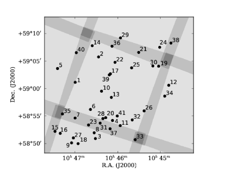
Our SMG sample consists of 38 of the 41 significant detections in the map (Lindner et al., 2011) of the LHN made using the Max Planck Millimeter Bolometer (MAMBO; Kreysa et al., 1998) array on the Institut de Radioastronomie Millimétrique telescope. We exclude one source that lacks a plausible radio counterpart (L20), one that has a likely X-ray counterpart (L26), and one nearby galaxy at (L29) from the stacking sample. Of our final sample of 38 galaxies, 37 (97%) have robust radio counterparts with a chance of spurious association (; Downes et al., 1986) of ; the remaining galaxy, L32, has . Stacking is performed with the coordinates of the SMGs’ radio counterparts, which have a mean offset of with respect to the SMG centroids. Five of our stacking targets have positions that are not listed in the catalog of Owen & Morrison (2008) because they had S/N (L9, L28, and L36), or they were blended together with nearby radio sources (L17 and L39) during extraction (Owen & Morrison, 2008; Lindner et al., 2011). The sample has a mean redshift of (see Table 1).
2.2 ACIS-I Observations
Our X-ray data are from the -pointing raster mosaic of the LHN obtained with the Advanced CCD Imaging Spectrometer (ACIS-I; Weisskopf et al., 1996) on the X-ray telescope by Polletta et al. (2006). The final mosaic comprises nine pointings arranged with overlap (see Figure 1). It covers a total area of and has a limiting conventional broad band (; 0.5-8.0) sensitivity of (Polletta et al., 2006). Fiolet et al. (2009) used these same data to search for a stacked X-ray signal among 33 -selected starburst galaxies, and found no significant –-band emission.
Within the sample of 41 MAMBO detections in the LHN, only L26 has a likely X-ray counterpart (CXOSWJ104523.6+585601) in the catalog of Wilkes et al. (2009). This X-ray source has conventional broad band (; 0.5-8.0), soft band (; 0.5–2.0), and hard band (; 2.0–8.0) X-ray fluxes of , , and , respectively, and a hardness ratio of . The hardness ratio is defined by , where and are the counts in the conventional hard and soft bands, respectively.
3 Stacking Analysis
In this section we describe our reduction of the X-ray data products and the methods used in our stacking analysis. We use two techniques: (1) image-based stacking in binned X-ray maps (§3.1), and (2) a photon-based spectral stacking procedure using optimized apertures (§3.2). The following subsections describe our implementation of these two methods.
3.1 Image-based stacking
We generate -pixel gridded maps of the total counts and effective exposure time in the , , and energy bands using the Interactive Analysis of Observations (CIAO; Fruscione et al., 2006) script fluximage. The characteristic energies input to fluximage to compute effective areas were , , and for the , , and bands, respectively. We then used the CIAO scripts reproject_image to merge the maps of each observation into one mosaic, and dmimgcalc to produce an exposure-corrected flux image in units of [photons ].
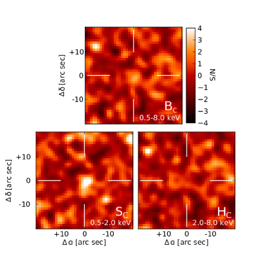
Figure 2 shows the resulting stacked image in each energy band. The S/N postage stamp images are shown with a color stretch from S/N= to . The peak S/N is 3.2, 4.8, and 2.0 in the , , and bands, respectively. The peak of the strong stacked detection in the band has an offset from the mean radio counterpart centroid position of .
3.2 Optimized broad-band stacking
Our second stacking technique does not use a binned X-ray map. Instead, we compute the stacked count rate and flux by directly counting photons at the stacking positions. The photometric aperture at each stacking location is derived using a technique similar to the optimized stacking algorithm presented in Treister et al. (2011, supplementary information).
The size and shape of the aperture at each stacking position is chosen to maximize the point-source S/N at that position on the ACIS-I chips. The apertures are constructed as follows. For each stacking position (shown in Figure 1), we (1) use the CIAO script mkpsf to generate a 2D image of the local PSF, (2) convolve this PSF with a Gaussian smoothing kernel (see below), and (3) find the enclosed-energy fraction (EEF) contour that maximizes the S/N of the flux within the aperture. The area enclosed by this contour defines the aperture. Because Poisson noise from the X-ray background is stronger than the flux at each position and the average exposure time does not change rapidly with increasing aperture size, the S/N within the aperture can be parametrized by as
| (1) |
where is the total area enclosed by the contour . This expression is the same as that derived by Treister et al. (2011), except that instead of using only circular apertures, we allow for non-axisymmetric apertures that follow the local shape of the PSF.
We compensate for the change in shape of the PSF with photon energy by generating two optimal apertures at each stacking position, one for each energy band (i.e., for characteristic energies of and ). Parts of the LHN mosaic were imaged multiple times due to the overlapping edges of the individual exposures (see Figure 1). For these positions we find the total effective aperture by maximizing Equation 1 using a linear combination of PSFs, one for each overlapping observation.
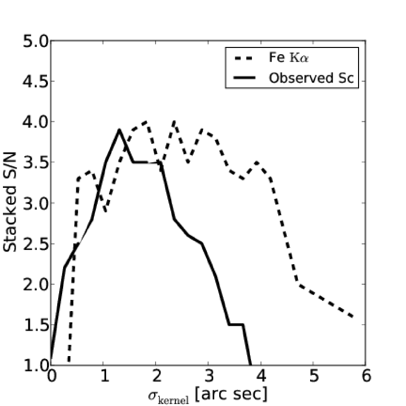
We broaden the local PSFs to accommodate photons that do not lie at the stacking centers due to intrinsic wavelength offsets in the galaxies and astrometric errors. Previous X-ray stacking analyses find the optimal aperture radius to be – (Lehmer et al., 2005; Georgantopoulos et al., 2011). We find similarly that our broad band stacked S/N is maximized with a smoothing kernel radius (see Figure 3), so we adopt this value for our subsequent broadband photometry. The smallest angular separation of any pair of stacking targets ( for L17 and L39) is larger than the maximum radial extent of the largest X-ray stacking aperture, so we can ignore the effects of X-ray blending within our sample.
The photons used for background subtraction are collected from arrays of large circular apertures positioned next to each stacking target position. The apertures are manually positioned to exclude any bright nearby X-ray sources that could contaminate the background estimate. To avoid possible systematic uncertainties associated with the background subtraction (see, e.g., Treister et al., 2011; Willott, 2011), we do not impose any S/N-based clipping or additional filtering in the background regions.
Table 3 shows the average stacked count rate and energy flux per galaxy in the three broad energy bands. We find a significant stacked detection in the soft band, and no significant detection in the hard band. To convert the stacked count rate into energy flux, we used the web-based CIAO Portable Interactive Multi-Mission Simulator111http://cxc.harvard.edu/toolkit/pimms.jsp (PIMMS- version 4.4; Cycle 5). The fluxes are corrected for Galactic absorption using the column density in the direction of the LHN center, (Stark et al., 1992). Our non-detection in the hard band leaves our calculation of the hardness ratio relatively unconstrained, (setting a limit on the photon index ), although it is clear that our sample has a steeply declining photon spectrum characteristic of star-forming galaxies (e.g., Ranalli et al., 2012). This estimate of HR was made after subtracting out the count rate in the soft band that is due to the strong Fe K line (see §3.3), which is a contribution for -broadened photometric apertures.
A high photon index of () is found by Laird et al. (2010), who stack on SCUBA-detected SMGs in the Deep Field North (CDF-N). An even steeper photon index of () is measured by Georgantopoulos et al. (2011), who stack on LABOCA-detected SMGs in the Extended Chandra Deep Field South (ECDF-S). We have used values of and to compute the stacked flux in each energy band (e.g., see Table 3), although the difference between the two estimates is less than the Poisson uncertainty (see Table 3).
3.3 Optimized spectral stacking
In addition to stacked broad-band fluxes, we also calculate the observed-frame and rest-frame stacked count-rate spectra for our sample.
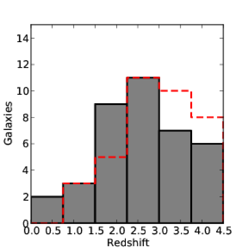
For each stacking target, we use redshift information in the following order of priority, subject to availablility: (1) spectroscopic (Polletta et al., 2006; Owen & Morrison, 2009; Fiolet et al., 2010), (2) -based photometric (Magdis et al., 2010; Roseboom et al., 2012), (3) -quality optical-based photometric (Strazzullo et al., 2010), and (4) millimeter/radio photometric estimated using the Carilli & Yun (1999) spectral index technique (Lindner et al., 2011). The redshift distribution of our sample is shown in Figure 4.
We use a flat sum of the observed counts at each stacking-target position with no weighting factors. Although this technique gives more weight to the brightest members of the stack, it is necessary given that of our stacking targets are individually detected and therefore S/N-based weights (used in, e.g., Treister et al., 2011) cannot be reliably assigned. For the rest-frame data, we separately coadd, blueshift, and bin the background photons to avoid creating artificial spectral features (see, e.g., Yaqoob, 2006).
The uncertainty in the rest-frame energy of the photons as a function of the observed photon energies due to the typical redshift error is estimated by the equation
| (2) |
This uncertainty is always larger than the energy resolution of the ACIS-I chips, so we set the rest-frame energy bin widths to match (Equation 2) using our sample’s average redshift and redshift uncertainty (see Table 2).
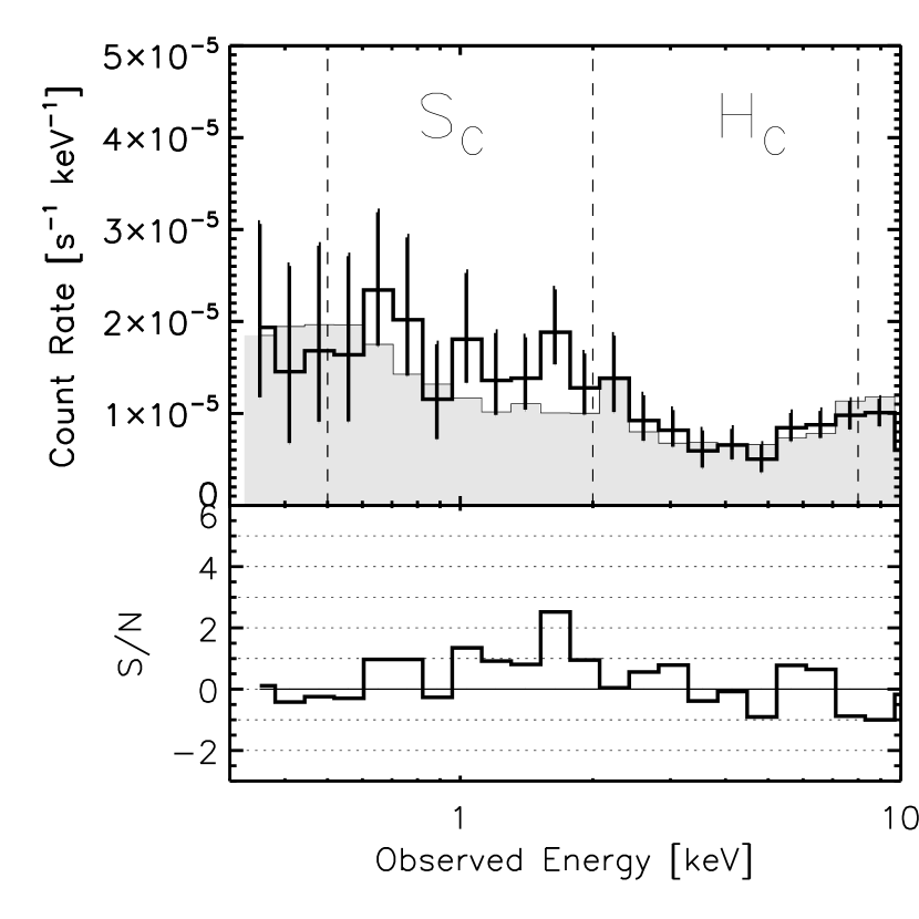
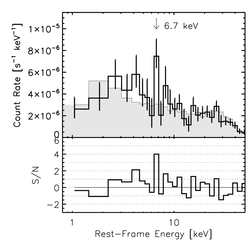
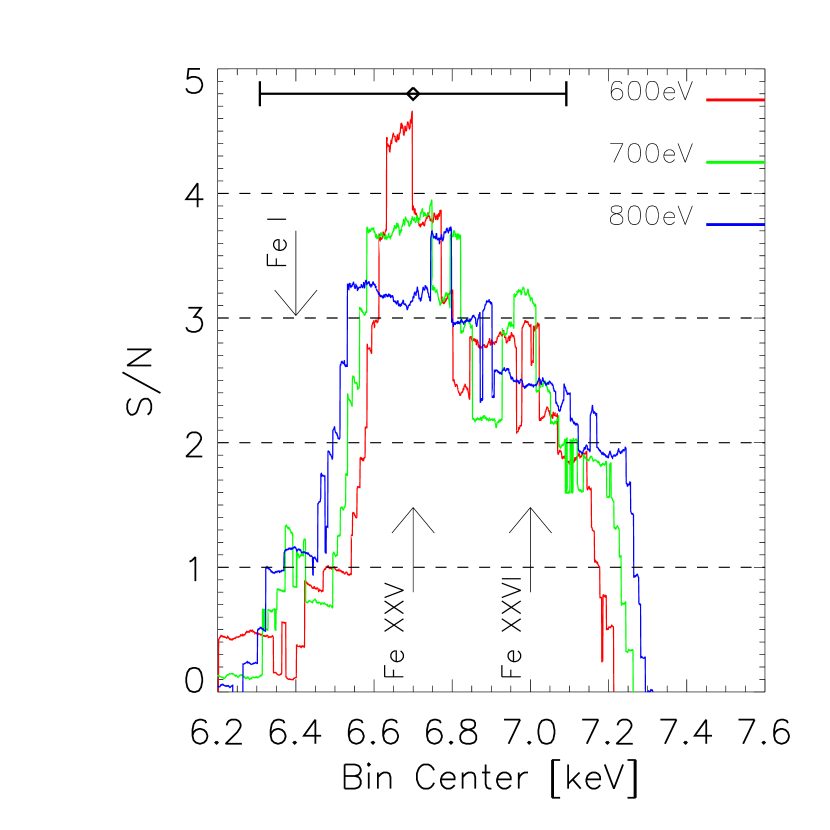
Figures 5 and 6 show the net observed and rest-frame count-rate spectra for our SMG sample, respectively. The rest-frame spectrum contains a emission feature with a centroid near , which we attribute to Fe K line emission from a mixture of Fe ionization states including Fe XXV (see §5.1.3). It is apparent from this rest-frame spectrum that a significant fraction of the observed soft-band flux is due to the Fe K emission line. If strong unresolved Fe K emission is a common feature in the X-ray spectra of other SMG samples, it may artificially lower their measured HR values by inflating their observed soft-band fluxes.
To ensure our stacking signal is not the result of contamination from a few strong targets, we performed a bootstrapping Monte Carlo analysis to recover the probability distribution for the single -energy bin (). The mean number of on-target counts in is 16, while the mean number of background counts in the bin is 8. Figure 7 shows that the resulting distribution closely matches that of an ideal Poisson distribution with a mean of 16, confirming that our stacking signal is characteristic of the entire sample, not a few outliers.
3.4 Estimating and
The mean stacked rest-frame hard-band X-ray luminosity, , of our sample is given by
| (3) |
where is the stacked energy flux per galaxy inside the observed – energy band (the energy band, redshifted by ), and is the luminosity distance at the redshift of each stacking target. We convert the observed count rate to an energy flux using PIMMS. The resulting rest frame X-ray luminosity is .
To estimate the equivalent width and line flux of the Fe K feature, we assume that the line emission is contained only within the single elevated bin at (see Figure 6) and estimate the local count-rate continuum around the feature by averaging together the 8 bins between 3–9 keV (excluding the bin containing the line). This results in an equivalent width of . Although the EW is relatively unconstrained, it is with 90% confidence. Using the nominal equivalent width and Equation A7, we find a mean stacked line flux of , and a mean line luminosity .
Figure 3 also shows that that the S/N of the Fe K signal only drops at a larger radius than the broad-band signal. If we interpret the X-ray continuum as originating from the galaxies’ nuclear regions, then this relative offset between the Fe K emission and the X-ray continuum indicates that the Fe K photons in our sample are systematically offset from the galaxies’ centers. By measuring the distance between the peaks of the two curves in Figure 3, we estimate the radial offset to be . For our computation of the Fe K line luminosity, we adopt an aperture broadening kernel suited to maximize the S/N of the Fe K emission line, .
We use a two-sample Kolmogorov-Smirnov (KS) test to determine the significance of the apparent angular extension of the Fe K emission relative to the continuum emission. First, we compute the PSF at the location of each stacking target, then sample the PSFs at the positions of their respective collections of optimally-selected photons (see §3.3). The PSFs are peak-normalized and smoothed by an amount to reflect intrinsic wavelength offsets and astrometric errors in the photon positions. We then compare the cumulative distributions of the observed soft-band (0.5–2.0) continuum photons (excluding those in the rest-frame Fe K bin) and the rest-frame Fe K photons using the two-sample KS test to determine with what confidence ( is the KS test significance) we can rule out the null hypothesis that the two samples are drawn from a common distribution. When using all 38 stacking positions, we find a maximum confidence of at (63 continuum counts and 15 Fe K counts). When we use only the stacking positions that have Fe K photon, the maximum confidence occurs at the same value of but has a reduced (29 continuum counts and 15 Fe K counts). Therefore, the extension in the Fe K emission relative to the continuum emission indicated by Figure 3 is a (71% confidence) effect, whose significance is limited primarily by the small number of Fe K photons.
4 Obscuration and Star Formation Rate
Two galaxies in our sample have [8–1000] estimated from Magdis et al. (2010), and 12 from Roseboom et al. (2012). For the remaining galaxies without SED fits, we estimate by scaling the SED from the nearby, bolometrically-star formation dominated ULIRG, :
| (4) |
in terms of
| (5) |
, the observed flux density , luminosity distance , target redshift , and redshift . The values for all stacking targets are presented in Table 1; the average value of our whole sample is
| (6) |
The mean radio luminosity density is calculated using our sample’s redshift distribution and flux densities (Owen & Morrison, 2008; Lindner et al., 2011):
| (7) |
We estimate the average star formation rate in our sample using the scaling relations of of Kennicutt (1998) in the infrared and Bell (2003) at radio wavelengths, giving and , respectively. These values are consistent with each other, but greater than the estimate using the X-ray scaling relation from Vattakunnel et al. (2012), . All three scaling relations assume a Salpeter (1955) initial mass function with limiting masses of 0.1 and . The SFR estimated using the X-ray luminosity may be low due to intrinsic absorption. We can derive a lower limit on the average absorbing column in our sample by computing how much obscuration is required to reduce the value of from an intrinsic value consistent with and . In this case, we would require based on our observed flux in the – band assuming and using . If we use this argument to estimate the X-ray luminosity, we find .
5 DISCUSSION
5.1 Comparison to previous surveys
In this section, we compare our results to those of previous X-ray analyses of SMG samples from the CDFN (Alexander et al., 2005b; Laird et al., 2010) and the (E)CDF-S (Georgantopoulos et al., 2011).
5.1.1 Detection rate
With only one significant X-ray counterpart in the LHN, the Lindner et al. (2011) SMG sample has an X-ray detection rate of . Alexander et al. (2005b) find a high X-ray detection rate of among SMGs and submillimeter-targeted radio galaxies (which constitute of their sample) in the CDFN. Laird et al. (2010) find a lower detection rate of using their purely submillimeter-selected sample derived from the inhomogenously covered SCUBA supermap (Borys et al., 2003). The LESS sample of Georgantopoulos et al. (2011) is also purely submillimeter-selected and has an X-ray detection rate of . However, unlike the SCUBA supermap, the LESS survey is produced with a single observing mode, and with uniform coverage.
We can place these four surveys in a common framework if we ask what fraction of SMGs in each survey have X-ray counterparts above the X-ray detection threshold in the LHN. In this case, we find 11 of 20 () for Alexander et al. (2005b), 0 of 35 () for Laird et al. (2010), and 11 of 126 () for Georgantopoulos et al. (2011). The latter two are in agreement with our sample in the LHN. These results indicate that a lower X-ray detection rate may be more characteristic of strictly submillimeter-detected SMGs from surveys made with uniform coverage.
5.1.2 vs. vs.
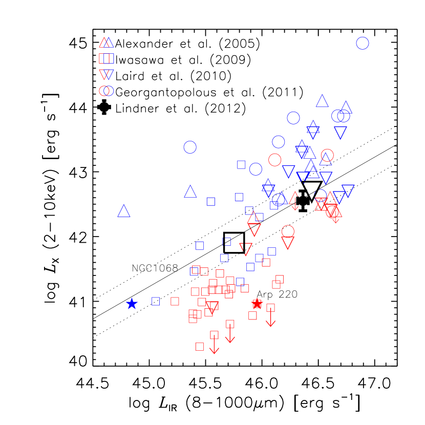
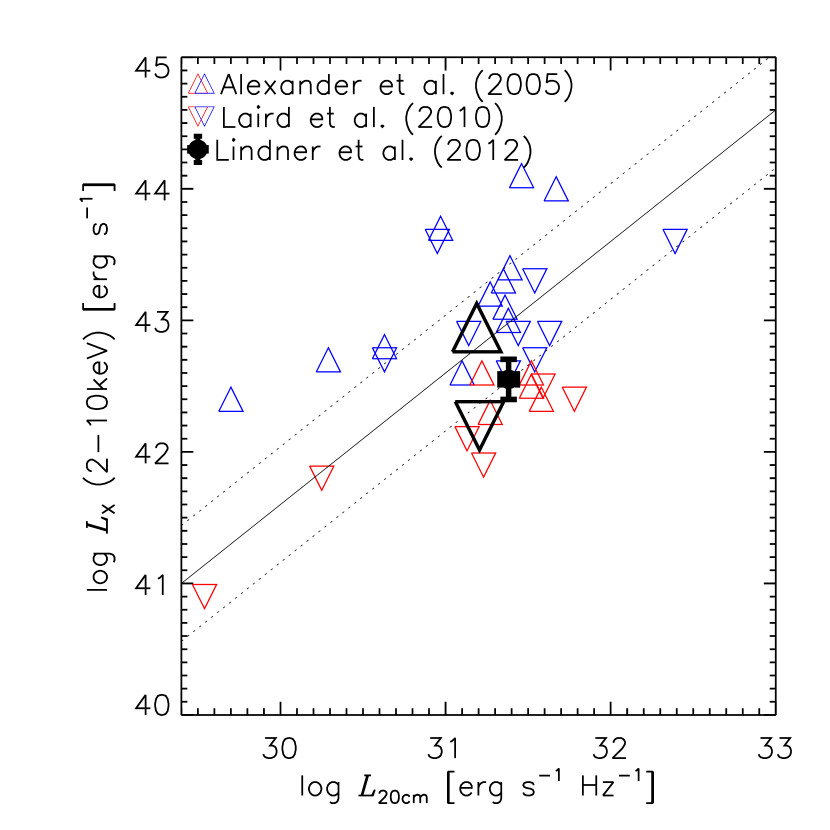
Figure 8 shows our sample’s average X-ray (corrected only for Galactic absorption), radio, and IR luminosities compared to those of other stacked SMG samples (Laird et al., 2010; Georgantopoulos et al., 2011), individually X-ray-detected SMGs (Alexander et al., 2005b; Laird et al., 2010; Georgantopoulos et al., 2011), and nearby LIRGs and ULIRGs (sample drawn from Iwasawa et al., 2009). Where available, we use the value from Table A2 of Pope et al. (2006) for the SMGs from the CDFN. For the twelve SMGs in Alexander et al. (2005b) that are not in the catalog of Pope et al. (2006), we scale using the average conversion factor for the eight SMGs common between the two samples, . The -detected SMGs from the (E)CDF-S are plotted with –. The local LIRGs and ULIRGs from Iwasawa et al. (2009) also have their – estimates scaled by . We also show the total sample luminosity average for Laird et al. (2010), including the contribution from their stacked SMGs that were not individually detected in the X-ray. The average properties of our stacking sample are in agreement with the total luminosities of Laird et al. (2010).
Figures 8 and 9 also indicate the AGN classification of each galaxy. Galaxies whose mid-IR or X-ray spectral properties are consistent with emission produced entirely by star formation are plotted in red, while those requiring the presence of an AGN are shown in blue. Georgantopoulos et al. (2011) divide their sample by using a probabilistic approach; those galaxies requiring the presence of a torus-dust component in their mid-IR SED according to an F-test are categorized as AGN. Laird et al. (2010) and Alexander et al. (2005b) separate out the AGN based on the most favored model of their X-ray spectra according to the Cash (1979) statistic. The sample of Iwasawa et al. (2009) is divided based on hardness ratio.
The division between AGN and non-AGN systems can be roughly determined based on the X-ray scaling relations of purely star-forming galaxies in the local universe (Ranalli et al., 2003; Vattakunnel et al., 2012), shown as solid black lines. The average properties of our stacking sample lie very near the Ranalli et al. (2003) relation. Considering the substantial intrinsic scatter in the spectral classifications of the Laird et al. (2010) sample, our stacking sample also probably contains a substantial fraction of both star-formation-only and AGN-required systems.
5.1.3 Fe K emission properties
The Fe K photons in our stacking sample may be more spatially extended than the continuum photons by (see §3.4). Extended and misaligned Fe K emission has been observed in Arp 220 (Iwasawa et al., 2005) and NGC 1068 (Young et al., 2001). We may also be blending together the emission from multiple components of merging systems of which only one component has strong Fe K emission (like, e.g., Arp 299; Ballo et al., 2004).
The bin width in our stacked rest-frame X-ray spectrum, which is set by the redshift uncertainties of our SMG sample, is larger than the rest energy separation between Fe K emission from neutral and highly-ionized iron (); therefore, it is difficult to determine the average Fe ionization fraction in our sample. Close inspection of the photons near the rest-frame Fe K line (see Figure 10) reveals a range of values between –, with a local maximum at . Given that the Fe line photons are contributed fairly evenly by the 38 targets in our stacking sample, and have been assigned to their bins based on a wide variety of redshift estimation techniques (spectroscopic, optical-photometric, -photometric, millimeter/radio-photometric), they are unlikely all to be systematically biased high or low. Therefore, a significant fraction of the detected Fe K photons likely originate from the highly-ionized species of Fe XXV or Fe XXVI. However, the rest-frame uncertainty in the energy of each photon implies an uncertainty in the centroid of the line profile of , insufficient to determine the relative fractions of each ionization state with certainty.
Strong emission () from highly ionized Fe K has been observed in the nearby ULIRG Arp 220 by Iwasawa et al. (2005) using . Iwasawa et al. (2009) also find strong emission () from the stacked spectrum of nearby ULIRGs (including Arp 220) that have no evidence of AGN emission (termed X-ray-quiet ULIRGs). Alexander et al. (2005b) detected strong () Fe K emission in the stacked SMG spectrum of the six SMGs in their sample with , and find that the line centroid is between and , indicating a substantial contribution from highly ionized gas.
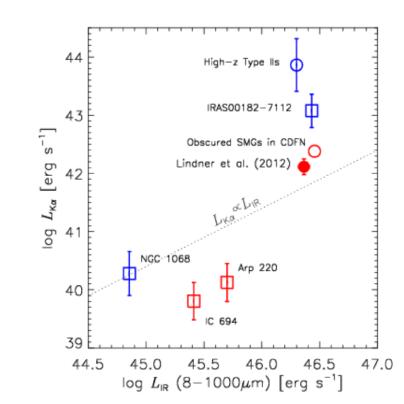
In Figure 11 we compare the relation between and in our sample with those for other individual systems and stacked samples with measured Fe K line luminosities and bolometrically dominant energy sources that are well understood. The dashed line represents a linear slope between and and has been normalized to NGC 1068, a nearby prototypical Seyfert II LIRG. Red symbols represent systems that do not have significant observed AGN bolometric contributions, like SMGs and local X-ray quiet ULIRGs; the blue symbols represent systems that have significant bolometric AGN contributions. Figure 11 shows that the relative Fe K/infrared luminosity fraction, , increases with increasing . If the Fe K emission is due to AGN activity, then this result may be in agreement with the observed trend that LIRGs/ULIRGs tend to be increasingly AGN-dominated with increasing (e.g., Tran et al., 2001).
5.2 Origin of the Fe K emission
This section discusses three possible physical origins for the Fe K emission detected in our stacked SMG sample: supernovae, galactic-scale winds, and AGNs. Because a significant fraction of our sample’s Fe K emission likely originates from the highly-ionized species Fe XXV (see, e.g., Figure 10) and because evidence for highly-ionized Fe K emission from other (U)LIRGs exists at both high (Alexander et al., 2005b) and low (e.g., Iwasawa et al., 2005) redshifts, the following sections focus on the origin of this high-ionization component.
5.2.1 Supernovae
Here we consider if the observed Fe K feature can be attributed to X-ray luminous supernovae. X-ray observations of the supernova SN 1986J in the nearby spiral galaxy NGC 831 reveal strong hard-band emission and a significant () line (Houck et al., 1998). Supernova 1986J decayed in the 2– band as from 1991 to 1996. We will take a conservative approach and use only the luminosity information in this time interval for our calculation. Given the X-ray luminosity and decay rate of SN 1986J (Houck et al., 1998), and assuming the star formation rate of our sample of order giving a supernova rate of , we would expect X-ray luminous supernovae to be visible at any given time. The combined supernova X-ray luminosity is therefore . Considering the fact that prior to 1991 SN 1986J was probably still dimming at a rate close to , this calculation is an underestimate. Therefore, supernovae like 1986J can satisfy the bolometric requirements for explaining the hard X-ray emission the Fe K line that we see in our stacked SMG sample.
However, if the supernovae associated with massive star formation are visible, then so must be high-mass X-ray binaries given the short time lifetimes of massive stars. These systems would dominate the hard X-ray emission from star-forming regions, and would severely dilute the Fe K emission (see, e.g., Iwasawa et al., 2009). We therefore rule out X-ray luminous supernovae and supernova remnants as the source of the Fe K emission in our sample.
5.2.2 Galactic-scale winds
As discussed in Iwasawa et al. (2005), who consider the emission line in Arp 220, a starburst-driven galactic-scale superwind of hot gas is energetically plausible as the source of the Fe K emission. Large outflows could also explain why the the Fe K line emission appears more extended than the X-ray continuum emission in our stacking sample. To explore this scenario, we used the X-ray spectral-fitting package XSPEC (Arnaud, 1996) to model an absorbed diffuse thermal X-ray (zphabs * mekal) spectrum and estimate the gas metallicity required to produce the strong high-ionization Fe K emission detected in our SMG sample. We computed the model EW values using the spectral window –, the same energy width as the bin containing the Fe K emission in our stacked rest-frame spectrum (Figure 6), which includes all Fe K ionization states. We fixed the gas temperature to Arp 220’s best-fit value (Iwasawa et al., 2005), the gas density to , the redshift to our sample’s average , and the obscuring hydrogen column density to (§4). Both the Fe K line luminosity and the continuum intensity vary linearly with , allowing us to express the relation between EW and as
| (8) |
where . EW is approximately proportional to for and approaches the constant value for . Because of this non-linear behavior, an abundance of can produce (90% confidence lower-limit) while a significantly greater abundance is needed to explain our nominal value . If a significant amount of our rest-frame 2–10 keV luminosity is from X-ray binaries, incapable of generating the observed line emission, then the required metallicity would be even higher. While the lower limit on our measured EW can be explained by thermal emission from a diffuse ionized plasma, especially considering the extreme enrichment taking place in systems like SMGs, generating an EW with a value close to our nominal measurement would require an unrealistic degree of high- enrichment.
5.2.3 AGN activity
AGNs hidden behind large hydrogen column densities may be responsible for the observed Fe K emission in our sample. The Fe K emission line is the signature spectral feature of the reprocessed (reflected) spectrum of an AGN (Matt et al., 2000). As the ionizing luminosity increases, so does the ionization fraction of the gas, shifting the dominant emission feature from (neutral and intermediate ionization states) to (helium-like Fe XXV) and (hydrogen-like Fe XXVI).
Some insight into the properties of SMGs can be gained from reviewing the well-studied Fe K emission properties of AGN and nearby ULIRGs. Strong () emission has been observed in systems that are bolometrically AGN-dominated, like IRAS 00182-7112 (Nandra & Iwasawa, 2007) and NGC 1068 (Young et al., 2001), as well as systems that appear to be energetically AGN-free, like Arp 220 (Iwasawa et al., 2005) and IC 694 (Ballo et al., 2004). However, direct evidence of a black hole accretion disk has been observed in Arp 220 by Downes & Eckart (2007) with the detection of a compact () continuum source in the center of the west nucleus torus. This source has a surface luminosity of , which is energetically incompatible with being powered by even the most extreme compact starbursts known. Only an accretion disk can be responsible for heating the dust. Highly ionized Fe K emission has also been observed in the AGN systems Mrk 273 (Balestra et al., 2005), NGC 4945 (Done et al., 2003), and NGC 6240 (Boller et al., 2003), along with a neutral Fe K component.
The narrow “cold” Fe K emission line is a ubiquitous feature in the spectra of optically-selected active galaxies out to high redshift (e.g., Corral et al., 2008; Iwasawa et al., 2011; Falocco et al., 2011). However, Iwasawa et al. (2011) also find evidence for highly ionized Fe K emission in two subsets of their X-ray selected AGN sample: Type I AGN with the highest Eddington ratios, and Type II AGN with the highest redshifts. The subsamples with highly ionized K emission show no evidence of a broad line Fe K feature; therefore, the highly-ionized Fe K photons probably do not originate from the accretion disk, but from more distant and tenuous outflowing gas. This scenario may also explain why the Fe K photons in our sample appear spatially extended with respect to the X-ray continuum photons.
A significant caveat is that it remains difficult to reconcile the power source required to produce offsets as large as in the photon distribution of our sample’s stacked Fe K emission (relative to the nuclear continuum; see §3.4) given the sample’s low average X-ray luminosity. For example, we can calculate the maximum radial distance out to which low-density gas can remain highly photoionized by a single ionizing source by assuming that our sample’s stacked infrared luminosity is produced by deeply-buried AGNs, i.e., . Using the ionization parameter ( is required for a significant Fe XXV ionization fraction: Kallman et al., 2004) with , we find . At our sample’s average redshift of , this corresponds to a typical angular offset of . Angular offsets larger than , like those tentatively indicated by our sample (see Figure 3), can be explained by SMGs that host multiple distributed ionizing sources. In particular, the radio continuum emission (defining our stacking positions) might be more closely associated with the X-ray continuum than with Fe K line emission in a complex, multi-component system. These results highlight the importance of resolving the sizes and morphologies of SMGs with high-resolution (sub)millimeter imaging (e.g., Tacconi et al., 2006).
If the high-ionization Fe K emission is ultimately due to star-formation processes (shocked gas from SNe), and the SFR is traced by the , then we should expect a linear relation between and . If the systems with the highest have an infrared contribution from obscured AGN that are not also emitting Fe K photons, then we would expect a slope that is even less than unity. However, Figure 11 shows that is relatively much more dominant in SMGs and high- AGN than in their lower-luminosity, lower-redshift analogues. This distinction indicates that highly ionized Fe K emission cannot be explained solely by star-formation processes and is more likely to be the result of AGN activity.
6 Conclusions
We analyze the X-ray properties of a complete sample of SMGs with radio counterparts from the LHN. This sample’s X-ray detection rate of is consistent with those for other uniformly-mapped, submillimeter-detected samples, considering the depth of our X-ray data. The X-ray undetected SMGs show a strong stacked detection in the band, and no significant detection in the band, similar to results from SMG stacking in the CDF-N (Laird et al., 2010) and CDF-S (Georgantopoulos et al., 2011).
We also use the available redshift information of our SMGs to compute the rest-frame, stacked count-rate spectrum of our sample. The rest-frame spectrum shows strong () emission from Fe K, possibly with contributions from Fe XXV and Fe XXVI. A comparison with other high-ionization Fe K-emitting systems from the literature indicates that accretion onto obscured AGNs is the likely explanation for the strong Fe K emission line. In our sample, the Fe K emission is responsible for of the observed soft-band X-ray flux. Therefore, if strong Fe line emission is a common feature in other SMG samples, it would significantly decrease the measured values of HR and lead to overestimates of the continuum spectral index .
We find a tentative indication (71% confidence) that our sample’s stacked distribution of Fe K photons is more spatially extended than that of the X-ray continuum. If confirmed by future studies, this result can help determine the physical origin of the prominent Fe K emission in SMGs.
Appendix A Detailed descriptions of calculations
A.1 Optimized spectral stacking method
We begin by labeling all the photons within the optimized apertures (see Section 3.1) of all of the stacking targets with the index , and those within the background regions for the targets . is the energy of the photon, and is the total effective exposure time in the mosaic at the position of . The notation refers to all the photons that have energies located the energy bin. The stacked mean count rate in the energy bin, , is then
| (A1) |
where is the aperture correction for the optimal aperture of the energy band of the photon. The background mean count rate in the bin is
| (A2) |
where is the ratio of the areas of the background region of the stacking position of the photon, and of the optimal aperture of that stacking position. It follows that the expected number of background counts in the bin, , is
| (A3) |
We use the double-sided 68%-confidence upper and lower limits, , and (Gehrels, 1986), to compute the count rate deviations in the bin due to the background, :
| (A4) |
Therefore, the net count rate density per galaxy in the bin, , is
| (A5) |
where is the width of the energy bin. We calculate the corresponding rest-frame spectrum by binning the photons according to their rest-frame energies, , where is the redshift of the stacking target associated with the photon.
A.2 Fe K energy flux
We use the CIAO script eff2evt to tabulate the local effective area (), and quantum efficiency (), for each photon in the on-target (background) apertures.
The mean stacked on-target and background photon fluxes in the bin, , and , are then
| (A6) |
and
| (A7) |
respectively.
References
- Alexander et al. (2003) Alexander, D.M., Bauer, F. E., Brandt, W. N. et al. 2003, AJ, 125, 383
- Alexander et al. (2005a) Alexander, D. M., Smail, I., Bauer, F. E., et al. 2005, Nature, 434, 738
- Alexander et al. (2005b) Alexander, D. M., Bauer, F. E., Chapman, S. C., et al. 2005, ApJ, 632, 736
- Arnaud (1996) Arnaud, K. A., 1996, Astronomical Data Analysis Software and Systems V, eds. Jacoby G. and Barnes J., p17, ASP Conf. Series Volume 101
- Balestra et al. (2005) Balestra, I., Boller, Th., Gallo, L., Lutz, D., & Hess, S. 2005, A&A, 442, 469
- Ballo et al. (2004) Ballo, L., Braito, V., Della Ceca, R., et al. 2004, ApJ, 600, 634
- Barger et al. (1998) Barger, A., Cowie, L., Sanders, D., et al. 1998, Nature, 394, 248
- Barger et al. (2001) Barger, A. J., Cowie, L. L., Steffen, A. T., et al. 2001, ApJ, 560, L23
- Bell (2003) Bell, E. F. 2003, ApJ, 586, 794
- Blain et al. (2002) Blain, A. W., Smail, I., Ivison, R. J., Kneib, J.P., & Frayer, T. 2002, Phys. Rep., 369, 111
- Boller et al. (2003) Boller, Th., Keil, R., Hasinger, G., et al. 2003, A&A, 411, 63
- Borys et al. (2003) Borys, C., Chapman, S., Halpern, M., & Scott, D. 2003, MNRAS, 344, 385
- Brandt et al. (2001) Brandt, W. N., Alexander, D. M., Hornschemeier, A. E., et al. 2001, AJ, 122, 2810
- Brusa et al. (2005) Brusa, M., Billi, R., & Comastri, A. 2005, ApJ, 621, L5
- Carilli & Yun (1999) Carilli, C. L., & Yun, M. S. 1999, ApJ, 513, L13
- Cash (1979) Cash, W. 1979, ApJ, 228, 939
- Chaudhary et al. (2010) Chaudhary, P., Brusa, M., Hasinger, G., Merloni, A., & Comastri, A. 2010, A&A, 518, A58
- Chapman et al. (2005) Chapman, S. C., Blain, A. W., Smail, I., Ivison, R. J. 2005, ApJ, 622, 772
- Corral et al. (2008) Corral, A., Page, M. J., Carrera, F. J., et al. 2008, A&A, 492, 71
- Done et al. (2003) Done, C., Madejski, G. M., Zycki, P. T., & Greenhill, L. J. 2003, ApJ, 588, 763
- Downes et al. (1986) Downes, A. J. B., Peacock, J. A., Savage, A., & Carrie, D. R. 1986, MNRAS, 218, 31
- Downes & Eckart (2007) Downes, D., & Eckart, A. 2007, A&A, 468, L57
- Falocco et al. (2011) Falocco, S., Carrera, F., Corral, A., et al. 2012, A&A, 538, 83
- Fiolet et al. (2009) Fiolet, N., Omont, A., Polletta, M., et al. 2009, å, 508, 117
- Fiolet et al. (2010) Fiolet, N., Omont, A., Lagache, G., et al. 2010, A&A, 524, A33
- Fruscione et al. (2006) Fruscione, A., McDowell, J. C., Allen, G. F., et al. 2006, Proc. SPIE, 6270, 62701V
- Gehrels (1986) Gehrels, N. 1986, ApJ, 303, 336
- Georgantopoulos et al. (2011) Georgantopoulos, I., Rovilos, E., & Comastri, A. 2011, A&A, 526, A46
- Holland et al. (1999) Holland, W. S., Robson, E. I., Gear, W. K., et al. 1999, MNRAS, 303, 659
- Houck et al. (1998) Houck, J., Bregman, J., Chevalier, R., & Tomisaka, K. 1998, ApJ, 493, 431
- Hughes et al. (1998) Hughes, D. H., Serjeant, S., Dunlop, J., et al. 1998, Nature, 394, 241
- Iwasawa et al. (2005) Iwasawa, K., Sanders, D. B., Evans, A. S., et al. 2005, MNRAS, 357, 565
- Iwasawa et al. (2009) Iwasawa, K., Sanders, D. B., Evans, A. S., et al. 2009, ApJ, 695, L103
- Iwasawa et al. (2011) Iwasawa, K., Sanders, D. B., Teng, S. H., et al. 2011, A&A, 529, A106
- Iwasawa et al. (2012) Iwasawa, K., Mainieri, V., Brusa, M., et al. 2012, A&A, 537, 86
- Kallman et al. (2004) Kallman, T. R., Palmeri, P., Bautista, M. A., Mendoza, C., & Krolik, J. H. 2004, ApJS, 155, 675
- Kennicutt (1998) Kennicutt, R. 1998, ARA&A, 36, 189
- Kreysa et al. (1998) Kreysa, E., Gemuend, H.-P., Gromke, J., et al. 1998, Proc. SPIE, 3357, 319
- Komatsu et al. (2011) Komatsu, E., Smith, K. M., Dunkley, J., et al. 2011, ApJS, 192, 18
- Laird et al. (2010) Laird, E. S., Nandra, K., Pope, A., & Scott, D. 2010, MNRAS, 401, 2763
- Lindner et al. (2011) Lindner, R. R., Baker, A. J., Omont, A., et al. 2011, ApJ, 737, 83
- Lehmer et al. (2005) Lehmer, B. D., Brandt, W. N., Alexander, D. M., et al. 2005, ApJ, 129, 1
- Lonsdale et al. (2003) Lonsdale, C. J., Smith, H., Rowan-Robsinson, M., et al. 2003, PASP, 115, 897
- Magdis et al. (2010) Magdis, G. E., Elbaz, D., Hwang, H., et al. 2010, MNRAS, 409, 22
- Matt et al. (2000) Matt, G., Fabian, A. C., Guainazzi, M., et al. 2000, MNRAS, 318, 173
- Menéndez-Delmestre et al. (2007) Menéndez-Delmestre, K., Blain, A., Alexander, D., et al. 2007, ApJ, 655, L65
- Menéndez-Delmestre et al. (2009) Menéndez-Delmestre, K., Blain, A., Smail, I., et al. 2009, ApJ, 699, 667
- Nandra & Iwasawa (2007) Nandra, K., & Iwasawa, K. 2007, MNRAS, 382, L1
- Owen & Morrison (2008) Owen, F. N., & Morrison, G. E. 2008, ApJ, 136, 1889
- Owen & Morrison (2009) Owen, F. N., & Morrison, G. E., 2009, ApJS, 182, 625
- Ozawa et al. (2009) Ozawa, M., Koyama, K., Yamaguchi, H., Masai, K., & Tamagawa, T. 2009, ApJ, 706, L71
- Pilbratt et al. (2010) Pilbratt, G. L., Riedinger, J. R., Passvogel, T., et al. 2010, A&A, 518, L1
- Polletta et al. (2006) Polletta, M., Wilkes, B., Siana, B., et al. 2006, ApJ, 642, 673
- Pope et al. (2006) Pope, A., Scott, D., Dickinson, M., Chary, R.-R., et al. 2006, MNRAS, 370, 1185
- Pope et al. (2008) Pope, A., Chary, R.-R., Alexander, D., et al. 2008, ApJ, 675, 1171
- Ranalli et al. (2003) Ranalli, P., Comastri, A., & Setti, G. 2003, A&A, 399, 39
- Ranalli et al. (2012) Ranalli, P., Comastri, A., Zamorani, G., et al. 2012, A&A, 542, A16
- Roseboom et al. (2012) Roseboom, I. G., Ivison, R. J., Greve, T. R., et al. 2012, MNRAS, 419, 2758
- Salpeter (1955) Salpeter, E. E. 1955, ApJ, 121, 161
- Sanders et al. (2003) Sanders, D. B., Mazzarella, J. M., Kim, D.-C., Surace, J. A., & Soifer, B. T. 2003, AJ, 126, 1607
- Smail et al. (1997) Smail, I., Ivison, R., & Blain, A. 1997, ApJ, 490, L5
- Spergel et al. (2007) Spergel, D. N., Bean, R., Doré, O., et al. 2007, ApJS, 170, 377
- Stark et al. (1992) Stark, A. A., Gammie, C. F., Wilson, R. W., et al. 1992, ApJS, 79, 77
- Strazzullo et al. (2010) Strazzullo, V., Pannella, M., Owen, F. N., et al. 2010, ApJ, 714, 1305
- Tacconi et al. (2006) Tacconi, L., J., Neri, R., Chapman, S. C., et al. 2006, ApJ, 640, 228
- Teng & Veilleux (2010) Teng, H., T. & Veilleux, S. 2010, ApJ, 725, 1848
- Tran et al. (2001) Tran, Q. D., Lutz, D., Genzel, R., et al. 2001, ApJ, 552, 527
- Treister et al. (2011) Treister, E., Schawinski, K., Volonteri, M., Natarajan, P., & Gawiser, E. 2011, Nature, 474, 356
- Valiante et al. (2007) Valiante, E., Lutz, D., Sturm, E., et al. 2007, ApJ, 660, 1060
- Vattakunnel et al. (2012) Vattakunnel, S., Tozzi, P., Matteucci, F., et al. 2012, MNRAS, 420, 2190
- Wall & Jenkins (2003) Wall, J. V., & Jenkins, C. R., 2003, Cambridge University Press, 130
- Wardlow et al. (2011) Wardlow, J. L., Smail, I., Coppin, K. E. K., et al. 2011, MNRAS, 415, 1479
- Wilkes et al. (2009) Wilkes, B. J., Kilgard, R., Kim, D.-W., et al. 2009, ApJS, 185, 433
- Willott (2011) Willott, C. J. 2011, ApJ, 742, L8
- Weiss et al. (2009) Weiss, A., Kovács, A., Coppin, K., et al. 2009, ApJ, 707, 1201
- Weisskopf et al. (1996) Weisskopf, M. C., O’dell, S. L., & van Speybroeck, L. P. 1996, Proc. SPIE, 2805, 2
- Yaqoob (2006) Yaqoob, T. 2006, Proceedings IAU Symposium No. 230, 461
- Young et al. (2001) Young, A. J., Wilson, A. S., & Shopbell P. L. 2001, ApJ, 556, 6

| ID | Name | RAaaPosition of radio counterpart | DecaaPosition of radio counterpart | typebbRedshift type: S = spectroscopic, P-IR = -based photometric, P-O = optical-based photometric, CY = estimated using the spectral index (Carilli & Yun, 1999). | referenceccReferences: P06 = Polletta et al. (2006), O09 = Owen & Morrison (2009), F10 = Fiolet et al. (2010), M10 = Magdis et al. (2010), S10 = Strazzullo et al. (2010), L11 = Lindner et al. (2011), R12 = Roseboom et al. (2012), L12 = This Work | dd8– | referenceccReferences: P06 = Polletta et al. (2006), O09 = Owen & Morrison (2009), F10 = Fiolet et al. (2010), M10 = Magdis et al. (2010), S10 = Strazzullo et al. (2010), L11 = Lindner et al. (2011), R12 = Roseboom et al. (2012), L12 = This Work | |
|---|---|---|---|---|---|---|---|---|
| J2000 | J2000 | |||||||
| L1 | 161.75083 | 59.018778 | 2.562 | S | P06 | 13.3 | R12 | |
| L2 | 161.61192 | 59.095778 | 4.09 | P-IR | R12 | 12.9 | L12 | |
| L3 | 161.63112 | 58.848889 | 1.8 | CY | L11 | 13.0 | L12 | |
| L4 | 161.53050 | 58.903889 | 4.4 | CY | L11 | 12.7 | L12 | |
| L5 | 161.85592 | 59.060139 | 3.00 | P-O | S10 | 13.1 | R12 | |
| L6 | 161.66112 | 58.936806 | 2.03 | S | F10 | 12.9 | R12 | |
| L7 | 161.75054 | 58.911500 | 2.74 | P-IR | R12 | 12.7 | L12 | |
| L8 | 161.63779 | 58.866417 | 2.07 | P-IR | R12 | 12.8 | L12 | |
| L9 | 161.77071 | 58.835750 | 3.9 | CY | L11 | 12.9 | L12 | |
| L10 | 161.59604 | 58.993000 | 3.01 | P-IR | R12 | 12.7 | L12 | |
| L11 | 161.48721 | 58.888556 | 1.95 | S | F10 | 12.9 | R12 | |
| L12 | 161.19829 | 59.009972 | 2.16 | P-O | S10 | 12.7 | R12 | |
| L13 | 161.53646 | 58.974583 | 0.32 | P-IR | R12 | 12.3 | L12 | |
| L14 | 161.64937 | 59.130139 | 2.26 | P-IR | R12 | 12.9 | R12 | |
| L15 | 161.86654 | 58.870583 | 2.78 | P-IR | R12 | 13.3 | R12 | |
| L16 | 161.83633 | 58.864722 | 3.24 | P-IR | R12 | 12.8 | L12 | |
| L17 | 161.54383 | 59.045000 | 2.65 | P-IR | R12 | 12.7 | L12 | |
| L18 | 161.73021 | 58.834444 | 2.15 | P-IR | R12 | 12.9 | L12 | |
| L19 | 161.25833 | 59.067583 | 4.1 | CY | L11 | 12.6 | L12 | |
| L20 | 161.57058 | 58.913694 | CY | L11 | – | – | ||
| L21 | 161.37575 | 59.110083 | 2.52 | P-IR | R12 | 12.6 | L12 | |
| L22 | 161.51763 | 59.080389 | 1.44 | P-IR | R12 | 12.3 | R12 | |
| L23 | 161.67129 | 58.890500 | 3.6 | CY | L11 | 12.6 | L12 | |
| L24 | 161.25279 | 59.126000 | 3.24 | P-O | S10 | 12.7 | R12 | |
| L25 | 161.41679 | 59.063333 | 3.5 | CY | L11 | 12.6 | L12 | |
| L26 | 161.34833 | 58.933611 | CY | L11 | – | – | ||
| L27 | 161.76000 | 58.850861 | 1.62 | P-IR | R12 | 12.7 | L12 | |
| L28 | 161.58804 | 58.909722 | 3.8 | CY | L11 | 12.5 | L12 | |
| L29 | 161.48129 | 59.154528 | 0.044 | S | O09 | 8.0 | R12 | |
| L30 | 161.29329 | 59.068639 | 0.71 | P-IR | R12 | 12.5 | L12 | |
| L31 | 161.60379 | 58.896444 | 2.90 | P-IR | R12 | 12.7 | R12 | |
| L32 | 161.41579 | 58.906917 | 2.40 | P-IR | M10 | 12.57 | M10 | |
| L33 | 161.39608 | 58.847139 | 2.63 | P-IR | R12 | 12.8 | L12 | |
| L34 | 161.22346 | 58.978194 | 2.46 | P-IR | R12 | 12.6 | L12 | |
| L35 | 161.82546 | 58.923833 | 2.14 | P-IR | R12 | 12.9 | L12 | |
| L36 | 161.53421 | 59.129444 | 4.5 | CY | L11 | 12.5 | L12 | |
| L37 | 161.54575 | 58.879139 | 1.72 | P-IR | M10 | 12.81 | M10 | |
| L38 | 161.18704 | 59.138361 | 3.6 | CY | L11 | 12.5 | L12 | |
| L39 | 161.55012 | 59.042583 | 2.59 | P-IR | R12 | 12.5 | L12 | |
| L40 | 161.74304 | 59.109306 | 0.78 | P-IR | R12 | 12.5 | L12 | |
| L41 | 161.50129 | 58.917944 | 1.49 | P-IR | R12 | 12.6 | L12 |
| Redshift type | N galaxies | References | |
|---|---|---|---|
| Spectroscopic | 3 | Polletta et al. (2006) | |
| Fiolet et al. (2010) | |||
| Owen & Morrison (2009) | |||
| Optical-based photometric | 3 | 0.2 | Strazzullo et al. (2010) |
| Infrared-based photometric | 23 | 0.4 | Magdis et al. (2010) |
| Roseboom et al. (2012) | |||
| Spectral index-based estimate | 9 | 0.6 | Lindner et al. (2011) |
| (Carilli & Yun, 1999) |
| Band | Energy | Net Rate | Flux () | Flux () | |
|---|---|---|---|---|---|
| keV | |||||
| 0.5–2.0 | – | ||||
| 2.0–8.0 | – | ||||
| 0.5–8.0 | – | ||||
| 0.55-2.22 | |||||
| 0.55-2.78 |
Note. — Unabsorbed fluxes calculated assuming the given photon index with Galactic absorption only. Hydrogen column density taken as that of the central Chandra pointing, (Stark et al., 1992). Luminosity calculation uses .