ABJ Triality: from Higher Spin Fields to Strings
Abstract:
We demonstrate that a supersymmetric and parity violating version of Vasiliev’s higher spin gauge theory in AdS4 admits boundary conditions that preserve or supersymmetries. In particular, we argue that the Vasiliev theory with Chan-Paton and boundary condition is holographically dual to the 2+1 dimensional ABJ theory in the limit of large and finite . In this system all bulk higher spin fields transform in the adjoint of the gauge group, whose bulk t’Hooft coupling is . Analysis of boundary conditions in Vasiliev theory allows us to determine exact relations between the parity breaking phase of Vasiliev theory and the coefficients of two and three point functions in Chern-Simons vector models at large . Our picture suggests that the supersymmetric Vasiliev theory can be obtained as a limit of type IIA string theory in AdS, and that the non-Abelian Vasiliev theory at strong bulk ’t Hooft coupling smoothly turn into a string field theory. The fundamental string is a singlet bound state of Vasiliev’s higher spin particles held together by gauge interactions. This is illustrated by the thermal partition function of free ABJ theory on a two sphere at large and even in the analytically tractable free limit. In this system the traces or strings of the low temperature phase break up into their Vasiliev particulate constituents at a deconfinement phase transition of order unity. At a higher temperature of order Vasiliev’s higher spin fields themselves break up into more elementary constituents at a deconfinement temperature, in a process described in the bulk as black hole nucleation.
1 Introduction and Summary
It has long been speculated that the tensionless limit of string theory is a theory of higher spin gauge fields. One of the most important explicit and nontrivial construction of interacting higher spin gauge theory is Vasiliev’s system in . It was conjectured by Klebanov and Polyakov [1], and by Sezgin and Sundell [2, 3], that the parity invariant A-type and B-type Vasiliev theories are dual to 2+1 dimensional bosonic and fermionic or vector models in the singlet sector. Substantial evidence for these conjectures has been provided by comparison of three-point functions [4, 5], and analysis of higher spin symmetries [6, 7, 8, 9].
It was noted in [10, 11] that, at large , the free and theories described above each have a family of one parameter conformal deformations, corresponding to turning on a finite Chern-Simons level for the or gauge group. It was conjectured in [11] that the bulk duals of the resultant Chern-Simons vector models is given by a one parameter family of parity violating Vasiliev theories. In the bulk description parity is broken by a nontrivial phase in function in Vasiliev’s theory that controls bulk interactions. This conjecture appeared to pass some nontrivial checks [11] but also faced some puzzling challenges [11]. In this paper we will find significant additional evidence in support of the proposal of [11] from the study of the bulk duals of supersymmetric vector Chern-Simons theories.
The duality between Vasiliev theory and 3d Chern-Simons boundary field theories does not rely on supersymmetry, and, indeed, most studies of this duality have been carried out in the non-supersymmetric context. However it is possible to construct supersymmetric analogues of the Type A and type B bosonic Vasiliev theories [12, 13, 14, 3, 15, 16]. With appropriate boundary conditions, these supersymmetric Vasiliev theories preserve all higher spin symmetries and are conjectured to be dual to free boundary supersymmetric gauge theories. In the spirit of [11] it is natural to attempt to construct bulk duals of the one parameter set of interacting supersymmetric Chern-Simons vector theories obtained by turning on a finite level for the Chern-Simons terms (recall that Chern Simons coupled gauge fields are free only in the limit ). Interacting supersymmetric Chern-Simons theories differ from their free counterparts in three ways. First, as emphasized above, their Chern-Simons level is taken to be finite. According to the conjecture of [11] this is accounted for by turning on the appropriate phase in Vasiliev’s equations. Second the Lagrangian includes potential terms of the schematic form and Yukawa terms of the schematic form , where and are fundamental and antifundamental scalars and fermions in the field theory. These terms may be regarded as double and triple trace deformations of the field theory; as is well known, the effect of such terms on the dual bulk theory may be accounted for by an appropriate modification of boundary conditions [17]. Lastly, supersymmetric field theories with and supersymmetry necessarily have two gauge groups with matter in the bifundamental. Such theories may be obtained by from theories with a single Chern-Simons coupled gauge group at level and fundamental matter by gauging a global symmetry with Chern-Simons level . In the dual bulk theory this gauging is implemented by a modification of the boundary conditions of the bulk vector gauge field [18].
These elements together suggest that it should be possible to find one parameter families of Vasiliev theories that preserve some supersymmetry upon turning on the parity violating bulk phase, if and only if one also modifies the boundary conditions of all bulk scalars, fermions and sometimes gauge fields in a coordinated way. In this paper we find that this is indeed the case. We are able to formulate one parameter families of parity violating Vasiliev theory (enhanced with Chan-Paton factors, see below) that preserve or supersymmetries depending on boundary conditions. In every case we identify conjectured dual Chern-Simons vector models dual to our bulk constructions.111A similar analysis of the breaking of higher spin symmetry by boundary conditions allows us to demonstrate that all deformations of type A or type B Vasiliev theories break all higher spin symmetries other than the conformal symmetry. We are also able to use this analysis to determine the functional form of the double trace part of higher spin currents that contain a scalar field.
The identification of parity violating Vasiliev theory with prescribed boundary conditions as the dual of Chern-Simons vector models pass a number of highly nontrivial checks. By considering of boundary conditions alone, we will be able to determine the exact relation between the parity breaking phase of Vasiliev theory, and two and three point function coefficients of Chern-Simons vector models at large . These imply non-perturbative relations among purely field theoretic quantities that are previously unknown (and presumably possible to prove by generalizing the computation of correlators in Chern-Simons-scalar vector model of [19] using Schwinger-Dyson 222See [11] for these equations in the Chern-Simons fermion model. equations to the supersymmetric theories). The results also agree with the relation between and Chern-Simons ’t Hooft coupling determined in [11] by explicit perturbative computations at one-loop and two-loop order.
From a physical viewpoint, the most interesting Vasiliev theory presented in this paper is the theory. It was already suggested in [11] that a supersymmetric version of the parity breaking Vasiliev theory in should be dual to the vector model limit of the ABJ theory, that is, a Chern-Simons-matter theory in the limit of large but finite . Since the ABJ theory is also dual to type IIA string theory in with flat -field, it was speculated that the Vasiliev theory must therefore be a limit of this string theory. The concrete supersymmetric Vasiliev system presented in this paper allows us to turn the suggestion of [11] into a precise conjecture for a duality between three distinct theories that are autonomously well defined atleast in particular limits.
The Vasiliev theory, conjectured below to be dual to theory has many elements absent in more familiar bosonic Vasiliev systems. First theory is ‘supersymmetric’ in the bulk. This means that all fields of the theory are functions of fermionic variables which obey Clifford algebra commutation relations (all bulk fields are also functions of the physical spacetime variables () as well as Vasiliev’s twistor variables , , , , as in bosonic Vasiliev theory). Next the star product used in the bulk equations is the usual Vasiliev star product times matrix multiplication in an auxiliary space. The physical effect of this maneuver is to endow the bulk theory with a gauge symmetry under which all bulk fields transform in the adjoint. Finally, for the reasons described above, interactions of the theory are also modified by a bulk phase, and bulk scalars, fermions and gauge fields obey nontrivial boundary conditions that depend on this phase.
The triality between ABJ theory, type IIA string theory on , and supersymmetric parity breaking Vasiliev theory may qualitatively be understood in the following manner. The propagating degrees of freedom of ABJ theory consist of bifundamental fields that we denote by and antibifundamental fields that we will call . A basis for the gauge singlet operators of the theory is given by the traces . As is well known from the study of ABJ duality, these single trace operators are dual to single string states. The basic ‘partons’ (the and fields) out of which this trace is composed are held together in this string state by the ‘glue’ of and gauge interactions.
Let us now study the limit . In this limit the glue that joins type fields to type fields (provided by the gauge group ) is significantly weaker than the glue that joins fields to fields (this glue is supplied by interactions). In this limit the trace effectively breaks up into weakly interacting particles , … . These particles, which transform in the adjoint of , are the dual to the adjoint fields of the dual Vasiliev theory. Indeed the spectrum of operators of field theory operators of the form precisely matches the spectrum of bulk fields of the dual Vasiliev system.
If our picture is correct, the fields of Vasiliev’s theory must bind together to make up fundamental IIA strings as is increased. We now describe a qualitative way in which this might happen. The bulk Vasiliev theory has gauge coupling , It follows that the bulk ’t Hooft coupling is . In the limit , the bulk Vasiliev theory is effectively weakly coupled. As increases, a class of multi-particle states of higher spin fields acquire large binding energies due to interactions, and are mapped to the single closed string states in type IIA string theory. Roughly speaking, the fundamental string of string theory is simply the flux tube string of the non abelian bulk Vasiliev theory.
Note that although we claim a family of supersymmetric Vasiliev theory with Chan-Paton factors and certain prescribed boundary conditions is equivalent to string theory on , we are not suggesting that Vasiliev’s equations are the same as the corresponding limit of closed string field equations. Not all single closed string states are mapped to single higher spin particles; infact the only closed strings that are mapped to Vasiliev’s particles are those dual to the operators of the form . Closed string field theory is the weakly interacting theory of the ‘glueball’ bound states of the Vasiliev fields; it is not a weakly interacting description of Vasiliev’s fields themselves.
We have asserted above that the glue between and partons is significantly weaker than the glue between and partons in the limit . This claim may be made quantitatively precise in a calculation in the ABJ theory with taken to be an arbitrary parameter. The computation in question is the partition function of free ABJ field theories on a sphere in the t’Hooft large and limit. We use the fact that the path integral that computes this partition function, even in the limit , is not completely free [20]. This path integral includes the effects of strong interactions between matter and the Polyakov line of and gauge fields. This computation of the partition function is a straightforward application of the techniques described in [20], but yields an interesting result (see Section 7, and see [21, 11] for related earlier work in the context of models with fundamental matter). We find that the theory undergoes two phase transitions as a function of temperature. At low temperature the theory is in a confined phase. This phase may be thought of as a gas of traces of the form , or, roughly, closed strings. Upon raising the temperature the field theory undergoes a first order phase transition at a temperature of order unity. Above the phase transition temperature, group deconfines while the group continues to completely confine333Throughout this paper we assume without loss of generality that . (we make this statement precise below.) The intermediate temperature phase has an effective description in terms of the partition function of a gauge theory whose effective matter degrees of freedom are simply the set of adjoint ‘mesons’ of the form . These adjoint degrees of freedom are deconfined. In other words the traces of the low temperature phase (dual to fundamental strings of ABJ theory) split up into a free gas of smaller - but not yet indivisible units, i.e. the fields of Vasiliev’s theory. Upon further raising the temperature, the theory undergoes yet another phase transition, this time of third order. This transition occurs at a temperature of order and is associated with the complete ‘deconfinement’ of the gauge group . At temperatures much higher than the second phase transition temperature, the system may be thought of as a plasma of the bifundamental and anti-bifundamental letters and . In other words the basic units, , of the intermediate temperature phase, split up into their basic building blocks in the high temperature phase. This extreme high temperature phase is presumably dual to a black hole in the bulk theory. 444In the very high temperature limit, this phase has recently been studied in closely related supersymmetric Chern Simons theories even away from the free limit [22] (generalizing earlier computations in nonsupersymmetric theories in [11].In the special case the intermediate phase never exists; the system directly transits from the string to the black hole phase. The fact that the deconfinement temperature is much smaller than the deconfinement temperature demonstrates that the glue between and type partons is much weaker than than between and type partons. Our computations also strongly suggests that the string dual to ABJ theory has a new finite temperature phase - one composed of a gas of Vasiliev’s particles - even at finite values of .
Let us note a curious aspect of the conjectured duality between Vasiliev’s theory and ABJ theory. The gauge groups and appear on an even footing in the ABJ field theory. In the bulk Vasiliev description, however, the two gauge groups play a very different role. The gauge group is manifest as a gauge symmetry in the bulk. However symmetry is not manifest in the bulk (just as the symmetry is not manifest in the bulk dual of Yang Mills); the dynamics of this gauge group that leads to the emergence of the background spacetime for Vasiliev theory. The deconfinement transition for is simply a deconfinement transition of the adjoint bulk degrees of freedom, while the deconfinement transition for is associated with the very different process of ‘black hole formation’. If our proposal for the dual description is correct, the gauged Vasiliev theory must enjoy an symmetry, which, from the bulk viewpoint is a sort of level – rank duality. Of course even a precise statement for the claim of such a level rank duality only makes sense if Vasiliev theory is well defined ‘quantum mechanically’ (i.e. away from small ) at least in the large limit.
We have noted above that Vasiliev’s theory should not be identified with closed string field theory. There may, however, be a sense in which it might be thought of as an open string field theory. We use the fact that there is an alternative way to engineer Chern-Simons vector models using string theory [23], that is by adding D6-branes wrapped on inside the , which preserves supersymmetry and amounts to adding fundamental hypermultiplets of the Chern-Simons gauge group. In the “minimal radius” limit where we send to zero, with flat -field flux , the geometry is entirely supported by the D6-branes [24].555We thank Daniel Jafferis for making this important suggestion and O. Aharony for related discussions. This type IIA open+closed string theory is dual to Chern-Simons vector model with hypermultiplet flavors. The duality suggests that the open+closed string field theory of the D6-branes reduces to precisely a supersymmetric Vasiliev theory in the minimal radius limit. Note that unlike the ABJ triality, here the open string fields on the D6-branes and the nonabelian higher spin gauge fields in Vasiliev’s system both carry Chan-Paton factors, and we expect one-to-one correspondence between single open string states and single higher spin particle states.
2 Vasiliev’s higher spin gauge theory in and its supersymmetric extension
The Vasiliev systems that we that we study in this paper are defined by a set of bulk equations of motion together with boundary conditions on the bulk fields. In this section we review the structure of the bulk equations. We turn to the consideration of boundary conditions in the next section.
In this section we first present a detailed review of bulk equations of the ‘standard’ Vasiliev theory. We then describe nonabelian and supersymmetric extensions of these equations. Throughout this paper we work with the so-called non-minimal version of Vasiliev’s equations, which describe the interactions of a field of each non-negative integer spin in . Under the AdS/CFT correspondence non-minimal Vasiliev equations are conjectured to be dual to gauged Chern-Simons-matter boundary theories.666 The non minimal equations admit a consistent truncation to the so-called minimal version of Vasiliev’s equations; this truncation projects out the gauge fields for odd spins and are conjectured to supply the dual to Chern-Simons boundary theories.
There are exactly two ‘standard’ non-minimal Vasiliev theories that preserve parity symmetry. These are the type A/B theories, which are conjectured to be dual to bosonic/fermionic vector models, restricted to the -singlet sector. Parity invariant Vasiliev theories are particular examples of a larger class of generically parity violating Vasiliev theories. These theories appear to be labeled by a real even function of one real variable. In subsection 2.1 we present a review of these theories. It was conjectured in [11] that a class of these parity violating theories are dual to Chern-Simons vector models.
In subsection 2.2 we then present a straightforward nonabelian extension of Vasiliev’s system, by introducing Chan-Paton factors into Vasiliev’s star product. The result of this extension is to promote the bulk gauge field to a gauge field; all other bulk fields transform in the adjoint of . The local gauge transformation parameter of Vasiliev’s theory is also promoted to a local matrix field that transforms in the adjoint of . The nature of the boundary CFT dual to the non abelian Vasiliev theory depends on boundary conditions. With ‘standard’ magnetic type boundary conditions for all gauge fields (that set prescribed values for the field strengths restricted to the boundary) the dual boundary CFT is obtained simply by coupling copies of (otherwise non interacting) matter multiplets to the same boundary Chern-Simons gauge field. The boundary theory has a ‘flavour’ global symmetry that acts on the identical matter multiplets.
In subsection 2.3 we then introduce the so called -extended supersymmetric Vasiliev theory (generalizing the special cases studied earlier in [12, 13, 14, 3, 15]). The main idea is to enhance Vasiliev’s fields to functions of fermionic fields (; we assume to be even) which obey a Clifford algebra777We emphasize that should not be confused with the number of globally conserved supercharges (equivalently is the number of supercharges in the superconformal algebra of the dual three-dimensional CFT). characterizes only the local structure of Vasiliev’s equations of motion. on the other hand depends on the choice of boundary condition for bulk fields of spin , and . As we will see is for parity violating Vasiliev theories, as expected from the dual CFT3 (, or course, can be arbitrarily large ). . This extension promotes the usual Vasiliev’s fields to dimensional matrices (or operators) that act on the dimensional representation of the Clifford algebra. The local Vasiliev gauge transformations are also promoted to functions of , and so matrices or operators888The bulk equations of motion the extended supersymmetric Vasiliev theory is identical to the theory extended by Chan Paton factors. However, the language of extended supersymmetric Vasiliev theory is more convenient when the boundary conditions of the problem break part of this symmetry, as will be the case later in this paper. . Half of the resultant fields (and gauge transformations) are fermionic; the other half are bosonic.
2.1 The standard parity violating bosonic Vasiliev theory
In this section we present the ‘standard’ non minimal Vasiliev equations, allowing, however, for parity violation.
2.1.1 Coordinates
In Euclidean space the fields of Vasiliev’s theory are functions of a collection of bosonic variables . () are an arbitrary set of coordinates on the four dimensional spacetime manifold. and are spinors under while and are spinors under a separate . As we will see below, Vasiliev’s equations enjoy invariance under local (in spacetime) rotations of , , and . This local rotational invariance, which, as we will see below is closely related to the tangent space symmetry of the first order formulation of general relativity, is only a small part of the much larger gauge symmetry of Vasiliev’s theory.
2.1.2 Star Product
Vasiliev’s equations are formulated in terms of a star product. This is just the usual local product in coordinate space; whereas in auxiliary space it is given by
| (2.1) | ||||
In the last line, the integral representation of the star product is defined by the contour for along in the complex plane, and along the contour . It is obvious from the first line of (LABEL:defstar) that ; this fact may be used to set the normalization of the integration measure in the second line. The star product is associative but non commutative; in fact it may be shown to be isomorphic to the usual Moyal star product under an appropriate change of variables. In Appendix A.1 we describe our conventions for lowering spinor indices and present some simple identities involving the star product.
Below we will make extensive use of the so called Kleinian operators and defined as
| (2.2) |
They have the property (see Appendix A.1 for a proof)
| (2.3) | ||||
2.1.3 Master fields
Vasiliev’s master fields consists of an -space 1-form
a -space 1-form
and a scalar , all of which depend on spacetime as well as the internal twistor coordinates which we denote collectively as . It is sometimes convenient to write and together as a 1-form on -space
will be regarded as a gauge connection with respect to the -algebra.
We also define
| (2.4) | ||||
Let be the exterior derivative with respect to the spacetime coordinates and denote by the exterior derivative with respect to the twistor variables . We will write . We will also find it useful to define the field strength
| (2.5) |
Note also that
| (2.6) |
2.1.4 Gauge Transformations
Vasiliev’s master fields transform under a large set of gauge symmetries. We will see later that the vacuum solution partially Higgs or breaks this gauge symmetry group down to a subgroup of large gauge transformations - either the higher spin symmetry group or the conformal group depending on boundary conditions.
Infinitesimal gauge transformations are generated by an arbitrary real function . By definition under gauge transformations
| (2.7) |
In other words the 1-form master field transforms as a gauge connection under the star algebra while transforms as a ‘twisted’ adjoint field. The operation that appears in (2.7) is defined as follows
Since does not involve differentials in , the action of on is equivalent to conjugation by , namely . ( acting on a 1-form in acts by conjugation by together with flipping the sign of ).
2.1.5 Truncation
The following truncation is imposed on the master fields and gauge transformation parameter . Define
We require
| (2.11) |
More explicitly, this is the statement that , and are even functions of whereas are odd in ,
| (2.12) |
A physical reason for the imposition of this truncation is the spin statistics theorem. As the physical fields of Vasiliev’s theory are all commuting, they must also transform in the vector (rather than spinor) conjugacy class of the tangent group; the projection (2.12) ensures that this is the case. One might expect from this remark that the consistency of Vasiliev’s equations requires this truncation; we will see explicitly below that this is the case.
2.1.6 Reality Conditions
It turns out that Vasiliev’s master fields admit two consistent projections that may be used to reduce their number of degrees of freedom. These two projections are a generalized reality projection (somewhat analogous to the Majorana condition for spinors) and a so called ‘minimal’ truncation (very loosely analogous to a chirality truncation for spinors). These two truncations are defined in terms of two natural operations defined on the master field; complex conjugation and an operation defined by the symbol . In this subsection we first define these two operations, and then use them to define the generalized reality projection. We will also briefly mention the minimal projection, even though we will not use the later in this paper.
Vasiliev’s fields master fields admit a straightforward complex conjugation operation, , defined by complex conjugating each of the component fields of Vasiliev theory and also the spinor variables 999As complex conjugation of interchanges left and right moving spinors, our definition of complex conjugation (the analytic continuation of the Lorentzian notion) must also have this property.
| (2.13) |
It is easily verified that
| (2.14) |
where is an arbitrary form and and arbitrary form. In other words complex conjugation commutes with the star and wedge product, without reversing the order of either of these products. Note also that the complex conjugation operation squares to the identity.
We now turn to the definition of the operation ; this operation is defined by
| (2.15) |
The signs in (2.15) are chosen101010Changing the RHS of (2.15) by an overall sign makes no difference to fields that obey (2.12) to ensure
| (2.16) |
(see (A.7) for a proof). In other words reverses the order of the product. Note however that by definition does not affect the order of wedge products of forms. As a consequence picks up an extra minus sign when acting on the product of two oneforms
(see (A.8) for a proof; the same equation is true if is a form and a form provided and are both odd; if atleast one of and is even we have no minus sign).
We now define the generalized reality projection that we will require Vasiliev’s master fields to obey throughout this paper (this projection defines the non-minimal Vasiliev theory which we study through this paper). The projection is defined by the conditions
| (2.17) |
The equality of the two different expressions supplied for in (2.17) follows upon using the fact commutes with (see (2.11)).
It is easily verified that (2.17) implies that
| (2.18) |
(see (A.13) for an expansion in components) and that
| (2.19) |
(2.17) may be thought of as a combination of two separate projections. The first is the ‘standard’ reality projection (see (A.9)). The second is the ‘minimal truncation’(A.10). As discussed in Appendix 2.12, it is consistent to simultaneously impose invariance of Vasiliev’s master field under both these projections. This operation defines the minimal Vasiliev theory (dual to Chern-Simons field theories). We will not study the minimal theory in this paper.
2.1.7 Equations of motion
Vasiliev’s gauge invariant equations of motion take the form
| (2.20) | ||||
where is a holomorphic function of , its complex conjugate, and the corresponding -function of . Namely, is defined by replacing all products of in the Taylor series of by the corresponding star products.
Note that both sides of the first of (LABEL:veqns) are gauge adjoints, while the second line of that equation transforms in the twisted adjoint. In Appendix A.4 we have demonstrated that the second equation of (LABEL:veqns) may be derived from the first (assuming that is a non-degenerate function) using the Bianchi identity
| (2.21) |
In Appendix A.4 we have also expanded Vasiliev’s equations in components to clarify their physical content. As elaborated in (LABEL:veqnsb) and (LABEL:veqnsc), it follows from (LABEL:veqns) that the field strength is flat and that the adjoint fields , and are covariantly constant. In addition, various components of these adjoint fields commute or anticommute with each other under the star product (see Appendix A.24 for a listing). The fields and , however, fail to commute with each other; their commutation relations are given by
| (2.22) |
2.1.8 Equivalences from field redefinitions
Vasiliev’s equations are characterized by a single complex holomorphic function . In this subsection we address the following question: to what extent to different functions label different theories?
Any field redefinition that preserves the gauge and Lorentz transformation properties of all fields, but changes the form of clearly demonstrates an equivalence of the theories with the corresponding choices of . The most general field redefinitions consistent with gauge and Lorentz transformations and the form of Vasiliev’s equations are
| (2.23) |
Several comments are in order. First note that the field redefinitions above obviously preserve form structure and gauge transformations properties. In particular these redefinitions preserve the fact that , and transform in the adjoint representation of the gauge group. Second the field redefinitions above are purely holomorphic (e.g. is a function only of but not of ). It is not difficult to convince oneself that this is necessary in order to preserve the holomorphic form of Vasiliev’s equations. Finally we have chosen to multiply the redefined functions and with functions from the right rather than the left. There is no lack of generality in this, however, as
| (2.24) | ||||
((LABEL:scomut) follows immediately from (A.24) derived in the Appendix). Finally, we have inserted a minus sign into the argument of the function for future convenience.
The reality conditions (2.17) impose constraints on the functions , and . It is not difficult to verify that is forced to be an odd real function . is forced to be odd because the complex conjugation operation turns into . When is odd, however, the truncation (2.11) may be used to turn back into . For instance, with , the field redefinition is
| (2.25) |
The RHS is still real because (it would not be real if were not odd).
In order to examine the constraints of (2.17) on the functions and note that
| (2.26) |
(where in the last step we have used (LABEL:scomut)). It follows that the redefined function obeys the reality condition (2.17) if and only if
where is the complex conjugate of the function .
The effect of the field redefinition of is simply to permit a redefinition of the argument of the function in Vasiliev’s equations by an arbitrary odd real function. The effect of the field redefinition of may be deduced as follows. The component of Vasiliev’s - the assertion that is a flat connection (see (LABEL:veqnsb)) - is clearly preserved by this field redefinition. The components of the equation asserts that and are covariantly constant. As and are also covariantly constant (see (LABEL:veqnsc)) the redefinition (2.23) clearly preserves this equation as well. However the components of the equations become
| (2.27) | ||||
Using (LABEL:scomut) and the fact that commutes with (this is obvious as and commute), these equations may be recast as
| (2.28) | ||||
(LABEL:hmp) is precisely the component of the Vasiliev equation (the third equation in (LABEL:veqnsb) ) with the replacement
| (2.29) |
or simply .
So we see that the theory is really defined by up to a change of variable for some odd real function and multiplication by an invertible holomorphic even function. Provided that the function admits a power series expansion about and that ,111111This condition can probably be weakend, but cannot be completely removed. For example if is an odd function, it is easy to convince oneself that it cannot be cast into the form (2.30). In this paper we will be interested in the Vasiliev duals to field theories. In the free limit, the dual Vasiliev theories to the field theory in question are given by of the form (2.30) with . It follows that, atleast in a power series in the field theory coupling, the Vasiliev duals to the corresponding field theories are defined by an that can be put in the form (2.30). in Appendix A.6 we demonstrate that we can can use these field redefinitions to put in the form
| (2.30) |
where is an arbitrary real even function.
Ignoring the special cases for which cannot be cast into the form (2.30), the function determines the general parity-violating Vasiliev theory.
2.1.9 The AdS solution
While Vasiliev’s system is formulated in terms of a set of background independent equations, the perturbation theory is defined by expanding around the vacuum. In order to study this solution it is useful to establish some conventions. Let and () denote the usual vielbein and spin connection one-forms on any space (the index transforms under the vector representation of the tangent space ). We define the corresponding bispinor objects
| (2.31) |
(see Appendix A.7 for definitions of the matrices that appear in this equation.) Let and be the vielbein and spin connection of Euclidean with unit radius. It may be shown that (see Appendix A.8 for some details)
| (2.32) | ||||
solves Vasiliev’s equations. We refer to this solution as the vacuum (as we will see below this preserves the invariance of space).
In the sequel we will find it convenient to work with a specific choice of coordinates and a specific choice of the vielbein field. For the metric on AdS space we work in Poincaré coordinates; the metric written in Euclidean signature takes the form
| (2.33) |
We also define the vielbein oneform fields
| (2.34) |
( runs over the index and ). The corresponding spin connection one form fields are given by
| (2.35) |
Using (2.31) we have explicitly
| (2.36) | ||||
Here our convention for contracting spinor indices is , etc (see Appendix A.7).
2.1.10 Linearization around AdS
The linearization of Vasiliev’s equations around the solution of the previous subsection, yields Fronsdal’s equations for the fields of all spins together with the free minimally coupled equation for an scalar field. The demonstration of this fact is rather involved; we will not review it here but instead refer the reader to [14, 25] for details. In this subsubsection we content ourselves with reviewing a few structural features of linearized solutions that will be of use to us in the sequel.
In the linearization of Vasiliev’s equations around , it turns out that the the physical degrees of freedom are contained entirely in the master fields restricted to . The spin- degrees of freedom are contained in
| (2.37) | ||||
for and . In particular, contains the rank- symmetric (double-)traceless (metric-like) tensor gauge field121212In order to formulate Fronsdal type equations with higher spin gauge symmetry of the form , the spin- gauge field is taken to be a rank- symmetric double-traceless tensor field . The trace part can be gauged away, however, leaving a symmetric rank- traceless tensor., and contain the self-dual and anti-self-dual parts of the higher spin generalization of the Weyl curvature tensor (and involve up to spacetime derivatives on the symmetric tensor field). While the components of and listed above are sufficient to recover all information about the spin fields, they are not the only components of the Vasiliev field that are turned on in the linearized solution. The linearized Vasiliev equations relate the components
| (2.38) | ||||
Starting from , the arrows (to the left as well as to the right) are generated by the action of derivatives. This may schematically be understood as follows. has symmetrized type and symmetrized type indices. Acting with the derivative , symmetrizing with all the type indices but contracting with one of the type indices yields an object with type indices but only type indices, taking us along the right arrow from in (LABEL:lefr). A similar operation, interchanging the role of dotted and undotted indices takes us along to the left.
The equations for the metric-like fields of the standard form can be extracted from Vasiliev’s equation by solving the auxiliary fields in terms of the metric-like fields order by order.
2.1.11 Parity
We wish to study Vasiliev’s equations in an expansion around space (with asymptotically boundary conditions, as we will detail in the next section). Consider the action of a parity operation. In the coordinates of (2.33) this operation acts as (for ). In order to fix the action of parity on the spinors , and and we adopt the choice of vielbein (2.34). With this choice the vielbein’s are oriented along the coordinate axes and the parity operator on spinors takes the standard flat space form . Using the explicit form for listed in (A.29), it follows that under parity
| (2.39) | ||||
(while the parity transformation of the oneform fields and are fixed by the transformations of and , the scalar can be either parity odd or parity even). With the choice of conventions adapted in Appendix A.7, . Consequently parity symmetry acts on by exchanging , , and so exchanges the two terms and in the equation of motion.
When are Vasiliev’s equations invariant under parity transformations? As we have seen above, may be either parity even or odd. Thus we need either or . Combined with (2.30), we have
| (2.40) |
They define the A-type and B-type Vasiliev theories, respectively.
Without imposing parity symmetry, however, the interactions of Vasiliev’s system is governed by the function , or the phase . If is not or , parity symmetry is violated. Parity symmetry is formally restored, however if we assign nontrivial parity transformation on (i.e. on the coupling parameters ) as well; there are two ways of doing this, with the scalar master field being parity even or odd:
| (2.41) | ||||
This will be useful in constraining the dependence of correlation functions on the coupling parameters .
2.1.12 The duals of free theories
The bulk scalar of Vasiliev’s theory turns out to have an effective mass in units of the AdS radius. Near the boundary in the coordinates of (2.33) the equation of motion the bulk scalar field to take the form
| (2.42) |
while the bulk vector field takes the form
| (2.43) |
In order to completely specify Vasiliev’s dynamical system we need to specify boundary conditions for the bulk scalar and vector fields (the unique consistent boundary condition of fields of higher spin is that they decay near the boundary like .) We postpone a systematic study of boundary conditions to the next section. In this subsubsection we specify the boundary conditions that define, respectively, the Vasiliev dual to the theory of free bosons and free fermions.
The type A bosonic Vasiliev theory with (for the unique bulk scalar) and (for the unique bulk vector field) is conjectured to be dual to the theory of a single fundamental boson coupled to Chern-Simons theory at infinite level . The primary single trace operators of this theory have quantum numbers
(the first label above refers to the scaling dimension of the operator, while the second label its spin), exactly matching the linearized spectrum of type A Vasiliev theory. In subsection 3.2 below we demonstrate that these are the only boundary conditions for the type A theory that preserve higher spin symmetry, the necessary and sufficient condition for these equations to be dual to the theory of free scalars [8].
The spectrum of primaries of a theory of free fermions subject to a singlet condition is given by
This is exactly the spectrum of the type B Vasiliev theory with boundary conditions . It is not difficult to convince oneself that these are the unique boundary conditions for the type B theory that preserve conformal invariance; in subsection 3.2 below that they also preserve the full the higher spin symmetry algebra, demonstrating that this Vasiliev system is dual to a theory of free fermions.
2.2 Nonabelian generalization
Vasiliev’s system in admits an obvious generalization to non-abelian higher spin fields, through the introduction of Chan-Paton factors, much like in open string field theory. We simply replace the master fields by matrix valued fields, and replace the -algebra in the gauge transformations and equations of motion by its tensor product with the algebra of complex matrices. In making this generalization we modify neither the truncation (2.11) nor the reality condition (2.17) (except that the complex conjugation in (2.17) is now defined with Hermitian conjugation on the matrices). We will refer to this system as Vasiliev’s theory with Chan-Paton factors.
One consequence of this replacement is that the gauge field in the bulk turns into a gauge field, and all other bulk fields are matrices that transform in the adjoint of this gauge group.
It is natural to conjecture that the non-minimal bosonic Vasiliev theory with Chan-Paton factors is then dual to vector model with flavors. Take the example of A-type theory in with boundary condition. The dual CFT is that of free massless complex scalars , , , restricted to the -singlet sector. The conserved higher spin currents are single trace operators in the adjoint of the global flavor symmetry. The dual bulk theory has a coupling constant . The bulk ’t Hooft coupling is then
| (2.44) |
We thus expect the bulk theory to be weakly coupled when . The latter will be referred to as the “vector model limit” of quiver type theories.
At the classical level the non abelian generalization of Vasiliev’s theory has different massless spin fields, and in particular different massless gravitons. This might appear to suggest that the dual field theory has exactly conserved stress tensors, in contradiction with general field theory lore for interacting field theories. In fact this is not the case. In Appendix A.9 we argue that effects lift the scaling dimension of all but one of the apparent stress tensors for every choice of boundary conditions except the one that is dual to a theory of decoupled free scalar or fermionic boundary fields.
2.3 Supersymmetric extension
To construct Vasiliev’s system with extended supersymmetry, we introduce Grassmannian auxiliary variables , , that obey Clifford algebra , and commute with all the twistor variables . By definition, the ’s do not participate in the -algebra. The master fields , as well as the gauge transformation parameter , are now all functions of ’s as well as of .
The operators may be thought of as matrices that act on an auxiliary dimensional ‘spinor’ space (we assume from now on that is even). Note that an arbitrary dimensional matrix can be written as a linear sum of products of matrices.131313This fact gives a map from the space of dimensional matrices to constant forms on an dimensional space, where is regarded as a basis one-form. Every dimensional matrix can be uniquely decomposed into the sum of a zero form , a one form , a two form an form . The number of basis forms is , precisely matching the number of independent matrix elements. Consequently at this stage the extension of Vasiliev’s system to allow for all fields to be functions of is simply identical to the non abelian extension of the previous subsection, for the special case . The construction of this subsection differs from that of the previous one in the truncation we apply on fields. The condition (2.11) continues to take the form
| (2.45) |
but with now defined as
| (2.46) |
and where
| (2.47) |
(note that and that it is still true that ).
While the modified truncation (2.45) looks formally similar to (2.11), it has one very important difference. As with (2.11) it ensures that those operators that commute with (i.e. are even functions of ) are also even functions of the spinor variables . However odd functions of , which anticommute with , are now forced to be odd functions of . Such functions transform in spinorial representations of the internal tangent space . Consequently, the new projection introduces bulk spinorial fields into Vasiliev’s theory, and simultaneously ensures that such fields are always anticommuting, in agreement with the spin statistics theorem.
The reality projection we impose on fields is almost unchanged compared to (2.17). We demand
| (2.48) |
The operation and the complex conjugation on the master fields, , are defined in the section 2.1, in combination with but reverses the order of the product of ’s, and ’s are real under complex conjugation. We require to reverse the order of in order to ensure that
(the reversal in the order of compensates for the sign picked up by the factor of under complex conjugation in (2.47)). The only other modification in (2.48) compared to (2.17) is in the factor on in the action on ; this additional factor is necessary in order for the two terms on the RHS of to be the same, after using the truncation equation (2.45), given that in this section has an additional factor of as compared to the bosonic theory.
Vasiliev’s equations take the form
| (2.49) | ||||
Compared to the bosonic theory, the only change in the first Vasiliev equation is the factor of in the argument of ; this factor is needed in order to preserve the reality of Vasiliev equations under the operation (2.48), as it follows from (2.48) that
The second Vasiliev equation is unchanged in form from the bosonic theory; however the operator is now taken to mean conjugation by together with , or equivalently, by the truncation condition (2.45) on the fields, conjugation by together with . Note in particular that
| (2.50) | ||||
As in the case of the bosonic theory, can generically be cast into the form by a field redefinition.
The expansion into components of the first of (LABEL:veqnss) is given by (LABEL:veqnsb), with the last line of that equation replaced by
| (2.51) |
The expansion in components of the second line of (LABEL:veqnss) is given by (LABEL:veqnsc) with no modifications.
As in the case of the bosonic theory, the second equation in (LABEL:veqnss) follows from the first using the Bianchi identity for the field strength. The details of the derivation differ in only minor ways from the bosonic derivation presented in Appendix A.4.141414(A.17) holds unchanged, (A.18) holds with these two equations are equivalent by (2.45). Equation (A.20) holds unchanged. (A.22) applies with . (A.23) holds unchanged.
Parity acts as
| (2.52) | ||||
The factor of in the last of (LABEL:susypar) is needed in order that the theory with is parity invariant.
2.4 The free dual of the parity preserving susy theory
In this subsection we consider the dual description of the parity preserving Vasiliev theory with appropriate boundary conditions. The equations we study have . Let us examine the bulk scalar fields which are given by the bottom component of the master field, namely , which obeys the truncation condition , i.e. is even in the ’s. There are real scalars, half of which are parity even, the other half parity odd. We impose boundary conditions to ensure that for the parity even scalars and for the parity odd scalars (see the next sections for details). In other words the fall off near the boundary is given by (2.42), with for parity even scalars, for all parity odd scalars. The boundary fall off for all gauge fields is given by (2.43) with .
The bulk theory has also has spin half bulk fermions, whose boundary conditions we now specify. Recall (see e.g. [26]) that the AdS/CFT dictionary for such fermions identifies the ‘source’ with the coefficient of the fall off of the parity even part of the bulk fermionic field (the same information is also present in the fall off of the parity odd part of the fermion field), while the ‘operator vev’ is identified with the coefficient of the of the parity odd part of the bulk fermion field (the same information is also present in the fall off of the parity even part of the fermion field). We impose the standard boundary conditions that set all sources to zero, i.e. we demand that the leading fall off of the fermionic field is entirely parity odd. We believe these boundary conditions preserve the fermionic higher spin symmetry (see section 5.4.1 for a partial verification) and so yield the theory dual to a free field theory.
The field content of this dual field theory is as follows; we have complex scalars in the fundamental representation and the same number of fundamental fermions (so that the singlets constructed out of bilinears of scalars or fermions match with the bulk scalars). We organize the fields in the boundary theory in the form
where is the index, are chiral and anti-chiral spinor indices of an global symmetry, and denotes the spacetime spinor index of . The singlet scalar operators, of dimension and , are
| (2.53) |
They are dual to the bulk fields (projected to the parity even and parity odd components, respectively)
| (2.54) |
The free CFT has bosonic flavor symmetry that act on the scalars and fermions separately, as well as complex fermionic symmetry currents
| (2.55) |
The Vasiliev bulk dual of the global symmetry is given by Vasiliev gauge transformations with independent of , or , but an arbitrary real even function of (i.e. an arbitrary even Hermitian operator built out of ). Operators of this nature may be subdivided into parity even and parity odd Hermitian operators which mutually commute. The parity even operators of this nature generate one factor of while the complementary parity even operators generate the second factor. The two central elements are generated by and respectively; these operators clearly commute with all even functions of , and so commute with all other generators, establishing their central nature.151515 As an example let us consider the case that is of particular interest to us below. The parity even is generated by while the parity odd is generated by (where ). It is easily verified that parity even Vasiliev scalars transform are neutral under the parity odd but transform in the adjoint of the parity even (the reverse statement is also true). On the other hand the parity even/odd spin half fields of Vasiliev theory transform in the (fundamental, antifundamental) and (fundamental, antifundamental), all in agreement with field theory expectations.
With the boundary conditions described in this section, the bulk theory may be equivalently written as the (i.e. minimally) extended supersymmetric Vasiliev theory with Chan-Paton factors and boundary conditions that preserved this symmetry. Our main interest in the bulk dual of the free theory, however, is as the starting point for the construction of the bulk dual of interacting theories. This will necessitate the introduction of parity violating phases into the theory and simultaneously modifying boundary conditions. The boundary conditions we will introduce break the global symmetry down to a smaller subgroup. In every case of interest the subgroup in question will turn out to be a subgroup of that is also a subgroup of the 161616As we will see in the sequel, we will find it possible to choose boundary conditions to preserve up to supersymmetries together with a flavour symmetry group which is a subgroup of . that rotates the ’s (here are the fermionic fields that enter Vasiliev’s construction, not the fermions of the dual boundary theory). As the preserved symmetry algebras have a natural action on , the language of extended supersymmetry will prove considerably more useful for us in subsequent sections than the language of the non abelian extension of the theory, which we will never adopt in the rest of this paper.
3 Higher Spin symmetry breaking by boundary conditions
In this technical section, we will demonstrate that higher spin bulk symmetries are broken by nontrivial values of the phase function and by generic boundary conditions.
In this section we study mainly the bosonic Vasiliev theory. We demonstrate that higher spin symmetry is broken by generic boundary conditions and generic values of the Vasiliev phase. Higher spin symmetry is preserved only for the type A and type B Vasiliev theories with boundary conditions described in subsection 2.1.12. We will see this explicitly by showing that, in every other case, the nonlinear (higher) spin- gauge transformation on the bulk scalar field, at the presence of a spin- boundary source, violates the boundary condition for the scalar field itself for every other choice of phase or boundary condition. We also use this bulk analysis together with a Ward identity to compute the coefficient in the schematic equation
where the RHS includes the contributions of descendants of and descendants of . The violation of the scalar boundary condition is directly related to a double trace term in the anomalous “conservation” law of the boundary spin- current, via a Ward identity.
This section does not directly relate to the study of the bulk duals of supersymmetric Chern Simons theories. Apart from the basic formalism for the study of symmetries in Vasiliev theory (see subsection 3.1 below) the only result of this subsection that we will use later in the paper are the identifications (3.28) and (3.31) presented below. The reader who is willing to take these results on faith, and who is uninterested in the bulk mechanism of higher spin symmetry breaking, could skip directly from subsection (3.1) to the next section.
3.1 Symmetries that preserve the AdS Solution
The asymptotic symmetry group of Vasiliev theory in is generated by gauge parameters that leave the vacuum solution (LABEL:adss) invariant. in the solution (LABEL:adss) is preserved if and only if the gauge transformation parameter is independent of , i.e it takes the form . As transforms homogeneously under gauge transformations, (in (LABEL:adss)) is preserved under arbitrary gauge transformations. The nontrivial conditions on arise from requiring that is preserved. For this to be the case is required to obey the equation
| (3.1) |
As the gauge field in the vacuum obeys the equation , is a flat connection and so may may be written in the “pure gauge” form.
| (3.2) |
where is the -inverse of . We may formally move to the gauge in which ;171717Note that the formal gauge transformation by is not a true gauge symmetry of the theory, as it violates the AdS boundary condition. We regard it as merely a solution generating technique. is preserved if and only if is independent of . Transforming back to the original gauge we conclude that the most general solution to (3.1) is given by of the form
| (3.3) |
where is independent of and is restricted, by the truncation condition, to be an even function of .181818This is obvious in the gauge in which vanishes. In the gauge (3.3) it follows from the truncation condition , and that the fact that , we see that .
The gauge function is not uniquely defined; it may be obtained by integrating the flat connection along a path from a base point to . We would then have and . See [27, 4] for explicit formulae for in Poincaré coordinates. We have used the explicit form of to obtain an explicit form for . We now describe our final result, which may easily independently be verified to obey (3.1)
Let us define . The -contraction between and is zero, and is nonzero only between and . Namely, we have
| (3.4) | ||||
In Poincaré coordinates, may be written in terms of as
| (3.5) |
A generating function for solutions to (3.1) is given by
| (3.6) | ||||
where , and are given in terms of constant spinors and by
| (3.7) | ||||
as defined in (3.6) may directly be verified to obey the linear equation (3.1). (3.6) is a generating function for solutions to that equation in the usual: upon expanding in a power series in the arbitrary constant spinors and the coefficients of different powers in this Taylor expansion independently obey (3.1) (this follows immediately from the linearity of (3.1)).
Notice that the various Taylor coefficients in (3.6) contains precisely all generating parameters for the universal enveloping algebra of (in the bosonic case) or its appropriate supersymmetric extension (in the susy case).
Let us first describe the bosonic case. Recall that, on the boundary, the conserved currents of the higher spin algebra may be obtained by dotting a spin conserved current with conformal killing vectors. Let us define the ‘spin charges’ as the charges obtained out of the spin conserved current by this dotting process. The spin- global symmetry generating parameter, , is then obtained from the terms in (3.6) of homogeneous degree in (or equivalently in and ).
As a special case consider the ‘spin two’ charges, i.e. the charges whose conserved currents correspond to the stress tensor dotted with a single conformal killing vector, i.e the conformal generators. These generators are quadratic in . These generators may be organized under the action of the boundary (i.e. the diagonal action of and ) as , corresponding to 3d angular momentum generators, momenta, boosts and dilations, in perfect correspondence with generators of the three dimensional conformal group .191919It may be checked that The Poincaré generators are obtained by simply setting to zero. Indeed the set of quadratic Hamiltonians in , with product defined by the star algebra, provides an oscillator construction of .
Let us now turn to the supersymmetric theory. The generators of the full extended superconformal algebra are given by terms that are quadratic in . Terms quadratic in are conformal generators. Terms quadratic in but independent of are symmetry generators. Terms linear in both and (we denote these by ) are supersymmetry and superconformal generators. More precisely the terms involving are Poincaré supersymmetry parameters, where the terms involving are special supersymmetry generators (in radial quantization with respect to the origin ).
In the sequel we will will make use of the following easily verified algebraic property of the generating function (3.6) under product,
| (3.8) | ||||
3.2 Breaking of higher spin symmetries by boundary conditions
Any given Vasiliev theory is defined by its equations of motion together with boundary conditions for all fields. Given any particular boundary conditions one may ask the following question: which of the large gauge transformation described in the previous subsection preserve these boundary conditions? In other words which if any of the gauge transformations have the property that they return a normalizable state (i.e. a solution of Vasiliev’s theory that obeys the prescribed boundary conditions) when acting on an arbitrary normalizable state? Such gauge transformations are genuine global symmetries of the system.
In this paper we will study the exact action of the large gauge transformations of the previous section on an arbitrary linearized solution of Vasiliev’s equations. The most general such solution may be obtained by superposition of the linearized responses to arbitrary boundary sources. Because of the linearity of the problem, it is adequate to study these sources one at a time. Consequently we focus on the linearized solution created by a spin source at on the boundary of . Such a source creates a response of the field everywhere in , and in particular in the neighborhood of the boundary at the point . We study the higher spin gauge transformations (for arbitrary ) on the master field at this point. The response to this gauge variation contains fields of various spins . As we will see below the response for always respects the standard boundary conditions for spin fields. However the same is not true of the response of the fields of low spins, namely , or . As we have seen in the previous section, for these fields it is possible to choose different boundary conditions, some of which turn out to be violated by the symmetry variation .
In the rest of this section we restrict our attention to the bosonic Vasiliev theory. The variation under an asymptotic symmetry generated by in (3.6) is given by (2.7).
Let be the spin- component of the linearized sourced by a current on the boundary, i.e. the boundary to bulk propagator for the spin- component of the master field with the source inserted at . only contains terms of order and , ; as we have explained above, the coefficients of these terms are spacetime derivatives of the basic spin field. We will work in Poincaré coordinates (2.33), with the spin- source located at . Without loss of generality, it suffices to consider the polarization tensor for , a three-dimensional symmetric traceless rank- tensor, of the form , for an arbitrary polarization spinor . The corresponding boundary-to-bulk propagator is computed in [4]. Here we generalize it slightly to the parity violating theory, by including the interaction phase , as
| (3.9) |
where and are defined as
| (3.10) |
Note that this formula is valid for spin , for the standard “magnetic” boundary condition in the case and for boundary condition in the case. The variation of under the asymptotic symmetry generated by is given by
where we made use of the properties (LABEL:epsid). Using the explicit expression of the boundary-to-bulk propagator, this is
| (3.11) | ||||
Note that although the source is a spin- current, there are nonzero variation of fields of various spins in . The self-dual part of the higher spin Weyl tensor, in particular, is obtained by restricting to . The variation of the self-dual part of the Weyl tensors of various spins are given by
| (3.12) | ||||
Now let us examine the behavior of near the boundary of . In the limit, the leading order terms in are given by
| (3.13) | ||||
The variation of the spin- Weyl tensor, , is extracted from terms of order in the above formula, which falls off like as . This is consistent with the boundary condition for fields of spin , independently of the phase . As promised above, the spin component of the response to an arbitrary gauge variation automatically obeys the prescribed boundary conditions for such field and so appears to yield no restrictions on allowed boundary conditions for the theory.
3.2.1 Anomalous higher spin symmetry variation of the scalar
The main difference between the scalar field and fields of arbitrary spin is that the prescribed boundary conditions for scalars involve both the leading as well as the subleading fall off of the scalar field. So while the leading fall off of the scalar field will never be faster than (in agreement with the general analysis above upon setting ), this is not sufficient to ensure that the scalar field variation obeys its boundary conditions.
Let us examine the variation of the scalar field due to a higher spin gauge transformation, at the presence of a spin- source at on the boundary. The spin component of the symmetry variation is given by (LABEL:deltabs) with set to zero,
| (3.14) | ||||
When expanded in a power series in , the RHS of (3.14) has the schematic form
Recall that the spin- symmetry variation (see the previous subsection for a definition) is extracted from terms of order in . It follows that we find a scalar response to spin gauge transformations only for . When this is the case (i.e. when is positive and even)
| (3.15) | ||||
Recall that , and , are arbitrary constant spinors. For generic parity violating phase , and with even , terms of order and are both nonzero, and so both and boundary conditions would be violated, leading to the breaking of spin- symmetry.
Note that the condition and that is even means that the broken symmetry has spin . In particular the conformal symmetries are never broken.212121Note that the extrapolation of this formula to the case assumes boundary to bulk propagator, and the variation is always consistent with the boundary condition.
The exceptional cases are when either or . These are precisely the interaction phase of the parity invariant theories. In the A-type theory, , we see that , and so boundary condition is preserved while boundary condition would be violated. This is as expected: the A-type theory with boundary condition is dual to the free or theory which has exact higher spin symmetry, whereas the A-type theory with boundary condition is dual to the critical theory, where the higher spin symmetry is broken at order . For the B-type theory, , we see that , and so the boundary condition is preserved, while boundary condition is violated. This is in agreement with the former case being dual to free fermions, and the latter dual to critical Gross-Neveu model where the higher spin symmetry is broken.
In summary, the only conditions under which any higher spin symmetries are preserved are the type A theory with or the type B theory with . These are precisely the theories conjectured to be dual to the free boson and free fermion theory respectively, in agreement with the results of [8].
3.2.2 Ward identity and current non-conservation relation
To quantify the breaking of higher spin symmetry, we now derive a sort of Ward identity that relates the anomalous spin- symmetry variation of the bulk fields, as seen above, to the non-conservation relation of the three-dimensional spin- current that generates the corresponding global symmetry of the boundary CFT.
Let us first word the argument in boundary field theory language. Let us consider the field theory quantity
where denote arbitrary current insertions away from the point , and denotes averaging with the measure of the field theory path integral. On the path integral we now perform the change of variables corresponding to a spin ‘symmetry’. Let denote the corresponding current. When is conserved this change of variables leaves the path integral unchanged in the neighborhood of (it acts on the insertions, but we ignore those as they are well separated from ). When the current is not conserved, however, it changes the action by . Let us suppose that
| (3.16) |
where is a differential operator, It follows that, in the large limit, the change in the path integral induced by this change of variables is given by
(where we have used the fact that the insertion of canonically normalized double trace operator contributes in the large limit only under conditions of maximal factorization). In other words the symmetry transformation amounts to an effective operator insertion of . Specializing to the case we conclude that, in the presence of a spin source , a spin symmetry transformation should turn on a non normalizable mode for the scalar field given by
| (3.17) |
Before proceeding with our analysis, we pause to restate our derivation of (3.26) in bulk rather than field theory language. Denote collectively by all bulk fields, and by a particular bulk field of some spin . Consider the spin- symmetry generated by gauge parameter , under which . Let be the renormalized boundary value of , namely as . Let us consider the expectation value of at the presence of some boundary source (of some other spin ) located away from . The path integral is invariant under an infinitesimal field redefinition , where takes the form of the asymptotic symmetry variation in the bulk, but vanishes for less than a small cutoff near the boundary, so as to preserve the prescribed boundary condition, . From this we can write
| (3.18) | ||||
The spin- source is subject to the transversality condition . Now should reduce to a boundary term,
| (3.19) |
where is a differential operator, and is the boundary current associated with the global symmetry generating parameter which is now a constant along the cutoff surface, which is then taken to . On the RHS of (3.19), we omitted possible higher order terms in the fields. From (3.18) we then obtain the relation
| (3.20) | ||||
Now specialize to the case , i.e. is the scalar field subject to the boundary condition such that the dual operator has dimension . The anomalous symmetry variation shows up in terms of order in . After integrating out using the two-point function of and taking the limit , we obtain the relation
| (3.21) |
Keep in mind that is the spin- transverse boundary source, and is the spin- global symmetry generating parameter. The differential operator appears in the spin- current non-conservation relation of the form
| (3.22) |
In particular, the double trace term on the RHS that involves a scalar operator takes the form
| (3.23) |
Knowing the LHS of (3.21) from the gauge variation of Vasiliev’s bulk fields, and using that fact that is given by the boundary two-point function of the spin- current, we can then derive using this Ward identity. In other words we have rederived (3.17).
(3.17) applies to arbitrary sources and also to arbitrary spin symmetry transformations. Let us assume that our sources is of the form specified in the previous subsection; all spinor indices on the source are dotted so with a constant spinor which is chosen so that
In other words our source is uniformly polarized in the direction. Let us also choose the spin variation to be generated by the current with
where is a constant vector. In other words we have chosen to specialize attention to those symmetries generated by the spin current contracted with translations in the direction rather than with a generic conformal killing vector. If we compare with the asymptotic symmetry variation the bulk scalar derived earlier we must set to zero and . It follows from the previous subsection that
| (3.24) | ||||
In the case, the anomalous variation comes from the order term in (3.24), giving
| (3.25) |
Here is a numerical constant that depends only on and .
(3.25) gives a formula for the appropriate term in (3.16) when the operators that appear in this equation have two point functions
| (3.26) |
Note in particular that these two point functions are independent of the phase . Let us now compare this relation to the results of Maldacena and Zhiboedov [9]. Those authors determined the non-conservation relation of currents of spin , which in the lightcone direction to take the form
| (3.27) |
where stands for double trace terms involving two currents of nonzero spins, total derivatives, and triple trace terms. Note that the first term we exhibited on the RHS of (LABEL:djsimp) is not a primary by itself, but when combined with the total derivatives term in becomes a double trace primary operator in the large limit. We have used the notation of [9] in the case of quasi-boson theory, but normalized the two-point function of to be independent of .
Indeed with , and the identification
| (3.28) |
the structure of the divergence of the current agrees with (3.25) obtained from the gauge transformation of bulk fields.
Similarly, in the case, the anomalous variation comes from the order term in (3.24). We have
| (3.29) |
This should be compared to the current non-conservation relation in the quasi-fermion theory, of the form
| (3.30) |
Once again, this agrees with the structure of (3.29), with , and the identification
| (3.31) |
Following the argument of [9], the double trace terms involving a scalar operator in the current non-conservation relation we derived from gauge transformation in Vasiliev theory allows us to determine the violation of current conservation in the three-point function, , and hence fix the normalization of the parity odd term in the three-point function.
Here we encounter a puzzle, however. By the Ward identity argument, we should also see an anomalous variation under global higher spin symmetry of a field of spin . This is not the case for our as computed in (LABEL:deltabs). Presumably the resolution to this puzzle lies in the gauge ambiguity in extracting the correlators from the boundary expectation value of Vasiliev’s master fields, which has not been properly understood thus far. This gauge ambiguity may also explain why one seems to find vanishing parity odd contribution to the three point function by naively applying the gauge function method of [5].222222We thank S. Giombi for discussions on this.
3.2.3 Anomalous higher spin symmetry variation of spin-1 gauge fields
Since one can choose a family of mixed electric-magnetic boundary conditions on the spin-1 gauge field in , such a boundary condition will generically be violated by the nonlinear asymptotic higher spin symmetry transformation as well.
Let us consider the self-dual part of the spin-1 field strength, whose variation is given in terms of , i.e. the terms in of order and independent of . According to (LABEL:bdryb), the leading order terms in , namely order terms, of in the presence of a spin- boundary source at is given by
| (3.32) | ||||
The anti-self-dual components, , is related by complex conjugation. Note that by the linearized Vasiliev equations with parity violating phase , and are related to the ordinary field strength of the vector gauge field by
| (3.33) | ||||
The factor here comes from the -dependence of the vielbein in . The two point functions of the operators dual to the gauge field in the equation above are given by
| (3.34) |
where is the bulk gauge coupling constant. The mixed boundary condition
is equivalent to232323In order to see this let us, for instance, take the special case . The relation becomes , so that
| (3.35) |
We see that precisely when or , the standard magnetic boundary condition, i.e. (), is consistent with higher spin gauge symmetry. For generic , however, there is no choice of for the boundary condition to be consistent with the higher spin symmetry variation on and . Therefore, we see again that the parity violating phase breaks all higher spin symmetries. From this one can also derive the double trace term involving a spin-1 current in the divergence of the spin- current of the boundary theory, using the method of the previous subsection.
4 Partial breaking of supersymmetry by boundary conditions
In this very important section we now turn to supersymmetric Vasiliev theory. We investigate the action of asymptotic supersymmetry transformations on bulk fields of spin 0, , and 1. As in the case of higher spin symmetries, we find that no supersymmetry transformation preserves generic boundary conditions. In other words generic boundary conditions on fields violate all supersymmetries. However we identify special classes of boundary conditions that that preserve and supersymmetries242424Theories with supersymmetry involve and gauge groups on the boundary. Such theories presumably have bulk duals in terms of the ‘minimal’ Vasiliev theory, which we, however, never study in this paper. We thank O. Aharony and S. Yokoyama for related discussions. in the next section. We go on present conjectures for CFT duals for these theories.
We emphasize that the boundary conditions presented in this section preserve supersymmetry when acting on linearized solutions of Vasiliev’s theory. The study of arbitrary linearize solutions is insufficient to completely determine the boundary conditions that preserve supersymmetry as we now explain.
Consider a linearized solution of a bulk scalar dual to an operator of dimension unity. The solution to such a scalar field decays at small like , and the boundary condition on this scalar asserts the vanishing of the term. However terms quadratic in are of at leading order, and so could potentially violate the boundary condition. It follows that the linearized boundary conditions studied presented in this section are not exact, but will be corrected at nonlinear order. Indeed we know one source of such corrections; the boundary condition deformations dual to the triple trace deformations of the dual boundary Chern Simons theory. We ignore all such nonlinear deformations in this section (see the next section for some remarks).
4.1 Structure of Boundary Conditions
Consider the -extended supersymmetric Vasiliev theory with parity violating phase . We already know that all higher spin symmetries are broken by any choice of boundary condition on fields of low spins, as expected for any interacting CFT. We also expect that any parity non-invariant CFT to have at most supersymmetry, and the question is whether the breaking of supersymmetries to in the -extended Vasiliev theory can be seen from the violating of boundary conditions by supersymmetry variations. The answer will turn out to be yes. In fact, we will be able to identify boundary conditions that preserve and supersymmetries, in precise agreement with the various -extended supersymmetric Chern-Simons vector models that differ from one another by double and triple trace deformations.
To begin we shall describe a set of boundary condition assignments on all bulk fields of spin , , and , that will turn out to preserve various number of supersymmetries and global flavor symmetries. The supersymmetry transformation of the bulk fields of spin , , and are derived explicitly in terms of the master field in Appendix B. For convenience we will speak of the -extended parity violating supersymmetric Vasiliev theory with no extra Chan-Paton factors, though our discussion can be straightforwardly generalized to include Chan-Paton factors. The bulk theory together with the prescribed boundary conditions are then conjectured to be holographically dual to supersymmetric Chern-Simons vector models with various number of supersymmetries and superpotentials.
4.1.1 Scalars
Vasiliev’s theory contains parity even scalar fields and an equal number of parity odd scalar fields. We expect the most general allowed boundary condition for these fields to take the form (5.6) (with set to zero, as we restrict attention to linear analysis in this section). If we view the collection of scalar fields as a linear vector space of dimension then (5.6) asserts that the component of scalars lies in a particular half dimensional subspace of this vector space, while the component of the scalars lies in a complementary half dimensional subspace (obtained from the first space by switching the role of parity even and parity odd scalars). Now the Vasiliev master field packs all scalars into a single even function of . In order to specify the boundary conditions on scalars, we must specify the dimensional subspace (of the dimensional space of even functions of ) that multiply in the small expansion of these fields. We must also choose out a half dimensional subspace of functions that multiply (as motivated above, this subspace will always turn out to be complementary to the first).
How do we specify the subspaces of interest? The technique we adopt is the following. We choose any convenient reference subspace that has the property that is the full space. Let be an arbitrary hermitian operator (built out of the fields) that acts on the subspace - i.e. is the exponential of a linear combination of projectors for the basis states of . An arbitrary real half dimensional subspace in the space of functions is given by . The complementary subspace (obtained by flipping parity even and parity odd functions) is given by . In other words the most general boundary conditions for the scalar part of takes the form
| (4.1) |
where and represent any function - not necessarily the same - that lie within the reference real half dimensional subspace on the space of functions of , and is an operator, to be specified, that acts on this subspace. It is not difficult to verify that (C.1) is consistent with the reality of . (C.1) may also be rewritten as
| (4.2) |
a form that makes the connection with (5.6) more explicit.
In the special case , and can be arbitrary (i.e. the reference half dimensional space can be chosen arbitrarily) and (C.1) simply asserts that parity odd scalars have dimension 1 while parity even scalars have dimension 2.
4.1.2 Spin half fermions
Boundary conditions for spin half fermions are specified more simply than for their scalar counterparts. The most general boundary condition relates the parity even part of any given fermion (the ‘source’) to the parity odd piece of all other fermions (‘the vev’). The most general real boundary condition of this form is that the spin- part of take the form
| (4.3) |
where is an arbitrary spinor and is an arbitrary hermitian operator (i.e. function of ). Reality of imposes .
In the limit these boundary conditions simply assert that the fall off of the fermion is entirely parity odd. Recall that according to the standard AdS/CFT rules, the parity even component of the fermion field may be identified with the expectation value of the boundary operator, while the parity odd part is an operator deformation. When (which in general is a linear operator that acts on , which are functions of ) is nonzero, the boundary conditions assert a linear relation between parity even and parity odd pieces, of the sort dual to a fermion-fermion double trace operator.
4.1.3 Gauge Fields
The electric-magnetic mixed boundary condition on the spin-1 field is
| (4.4) |
Here is equal to for the magnetic boundary condition, corresponding to ungauged flavor group in the boundary CFT (recall that is identified with the bulk Maxwell field strength; see above). Once again is, in general, an operator that acts on . Reality of gives
We will see that the and boundary conditions requires taking to be a nontrivial linear operator that acts on , which amounts to gauging a flavor group with a finite Chern-Simons level.
Now to characterize the boundary condition, we simply need to give the linear operators , , which act on , , , and a set of linear conditions on .
We now proceed to enumerate boundary conditions that preserve different degrees of supersymmetry. In each case we also conjecture a field theory dual for the resultant Vasiliev theory. For future use we present the Lagrangians of the corresponding field theories in Appendix D.
4.2 The theory with two chiral multiplets
Let us start with extended supersymmetric Vasiliev theory. The master fields depend on the auxiliary Grassmannian variables . With , and in the fermion and scalar boundary conditions, respectively, the dual CFT is the free theory of 2 chiral multiplets (in language) in the fundamental representation of , with a total number of 16 supersymmetries. Now we will turn on nonzero , and describe a set of boundary conditions that preserve supersymmetry (4 supercharges) and flavor symmetry. The boundary condition for the spin-1 field is the standard magnetic one. The boundary condition for spin- and spin-0 fields are given by (B.10), (B.11), (B.18), with
| (4.5) |
where stands for the projection onto the subspace spanned by the monomials ; are subject to the constraint that they commute with , or equivalently, are spanned by . The 2 supersymmetry parameters are given by , , with
| (4.6) |
where . is a constant Grassmannian spinor parameter that anti-commutes with all ’s.
Clearly, with , (LABEL:VspV) obeys the fermion boundary condition (B.10), (B.11), and (LABEL:FspF) obeys the magnetic boundary condition on the spin-1 fields (B.1), (B.2). (LABEL:fermiontoboson) with obeys (B.18) with of the form , or , both of which commute with . Finally, in the RHS of (LABEL:VgbV), all commutators of vanish, leaving the terms with anti-commutators only, which satisfy (C.21), (B.11) with . Clearly, an flavor symmetry rotating is preserved by this boundary condition.
It is natural to propose that the extended parity violating Vasiliev theory with this boundary condition is dual to Chern-Simons vector model with 2 fundamental chiral multiplets. There is no gauge invariant superpotential in this case, while there is an flavor symmetry252525Note that the field theory is left invariant under a larger set of transformations, which rotates the chiral multiplets into each other. However the diagonal in acts in the same way on all fundamental fields, and so is part of the gauge symmetry. There is nonetheless a bulk gauge field - with content I -formally corresponding to this factor. rotating the two chiral multiplets, which is identified with the symmetry of rotations in , and preserved by the boundary conditions listed above.
Let us elaborate on, for instance, the scalar boundary conditions. There are a total of eight scalars in the problem (the number of even functions of ). A basis for parity even scalars is given by and where . A basis for parity odd scalars is given by and . In each case the scalars transform in the of . Recall that the fundamental fields of the field theory (scalars as well as fermions) transform in the of the flavour symmetry ; it follows that bilinears in these fields also transform in the of , establishing a natural map between bulk fields and field theory operators.
The boundary conditions (4.5) assert that the coefficient of the term of the parity even scalars/vectors is equal to times the coefficient of the of the corresponding parity odd scalars/vectors. Similarly the coefficient of the term of the parity odd scalars/vectors is equal to times the coefficient of the of the corresponding parity even scalars/vectors. This is exactly the kind of boundary condition generated by a double trace deformation that couples the dual dimension one and dimension two operators, with equal couplings in the scalar and vector (of ) channels. We will elaborate on this in much more detail in the next section.
4.3 A family of theories with two chiral multiplets
If we keep only the supersymmetry generator given by
| (4.7) |
then a one-parameter family of boundary conditions that preserve supersymmetry is given by
| (4.8) |
where and are the projection operators that projects an odd function of ’s onto the subspaces spanned by
| (4.9) |
and
| (4.10) |
respectively. is now an arbitrary phase (independent of ).
This family of boundary conditions is dual to deformations of the theory with two chiral flavors, by turning on an (non-holomorphic) superpotential that preserves the flavor symmetry (corresponding to the bulk symmetry that rotates ).
The same theory can also be rewritten as the extended supersymmetric Vasiliev theory with matrix extension. The spin-1, fermion, and scalar boundary conditions are given by
| (4.11) |
It is natural to wonder about the relationship between the parameter above and the field theory parameter (see (D.7)). General considerations leave this relationship undetermined; however we will present a conjecture for this relationship in the next section.
4.4 The theory with a chiral multiplet and a chiral multiplet
Now let us describe a boundary condition that preserve the two supersymmetries generated by
| (4.12) |
It is given by
| (4.13) |
where stands for the projection onto the subspace spanned by the monomials , as before; are now subject to the constraint that they commute with either or , i.e. are spanned by , , , , . Note that when acting on the latter four monomials, vanishes, and and may be replaced by and . Therefore, only half of the components of are independent, as required. One can straightforwardly verified that this set of boundary conditions preserve the two supersymmetries (4.12). Clearly, the flavor symmetry that rotates is still preserved, but there is no flavor symmetry. We also have the R symmetry corresponding to rotations of .
The Vasiliev theory with this boundary is then naturally proposed to be dual to Chern-Simons vector model with a fundamental and an anti-fundamental chiral flavor, with flavor symmetry 262626 One of these two factors is actually part of the gauge group and so acts trivially on all gauge invariant operators. (corresponding to the components of the bulk vector gauge field proportional to 1 and ) besides the R-symmetry, which means that the superpotential vanishes, since a nonzero superpotential would break the flavor symmetry to a single .
4.5 A family of theories with a chiral multiplet and a chiral multiplet
The boundary condition in the above section is a special point inside a one-parameter family of boundary conditions which preserved the same set of supersymmetries. It is given by
| (4.14) | ||||
This one-parameter family of deformations is naturally identified with the superpotential deformation of the Chern-Simons vector model with a fundamental and an anti-fundamental chiral flavor. This superpotential is marginal at infinite ; at finite there are two inequivalent conformally invariant fixed points [28]. The point is the boundary condition on the above section, describing the theory with no superpotential, whereas give the point, as will be discussed in the next subsection.
4.6 The theory
The boundary condition that preserve supersymmetry generated by the parameters
| (4.15) |
is given by
| (4.16) |
This boundary condition is dual to the Chern-Simons vector model with a single fundamental hypermultiplet, which may be obtained from the theory with a fundamental and an anti-fundamental chiral multiplet by a turning on a superpotential. The symmetry of rotations in , and maps to the R-symmetry of the model. Notice that unlike the case studied in section 4.2, reflecting the fact that the R symmetry, unlike a flavor symmetry, acts differently on bosons and fermions.
4.7 The theory
The boundary condition that preserve supersymmetry generated by the parameters
| (4.17) |
is given by
| (4.18) |
are subject to the constraint
| (4.19) |
Note also that the components of proportional to are subject to the projection also, as follows automatically from (C.1), (4.2). The boundary conditions above are invariant under the R symmetry of rotations in , , and .
This boundary condition is dual to the Chern-Simons quiver theory with gauge group and a single bi-fundamental hypermultiplet. The latter can be obtained from the Chern-Simons vector model with one hypermultiplet flavor by gauging the flavor current multiplet with another Chern-Simons gauge field at level [29].
4.8 An one parameter family of theories
4.9 The theory
To construct the bulk dual of the ABJ vector model [30, 31], we need to double the number of matter fields in the boundary field theory, and correspondingly quadruple the number of bulk fields. This is achieved with the extended supersymmetric Vasiliev theory, which in the parity even case (dual to free CFT) can have up to 64 supersymmetries. We are interested in the parity violating theory, with nonzero interaction phase , with a set of boundary conditions that preserve supersymmetries, generated by the parameters
| (4.21) |
Similarly to the theory with one hypermultiplet, here we need to take the boundary condition on the bulk spin-1 field to be
| (4.22) |
The spin- and spin-0 boundary conditions are given by
| (4.23) |
where for instance stands for the projection onto the subspace spanned by all ’s, . are subject to the constraint
| (4.24) |
which projects out half of the components of . Note that these boundary conditions enjoy invariance under the R symmetry rotations of the coordinates.
By comparing the difference between and with the Chern-Simons level of what would be the flavor group of the Chern-Simons vector model with two hypermultiplets, we will be able to identify in terms of below.
4.10 Another one parameter family of theories
5 Deconstructing the supersymmetric boundary conditions
5.1 The goal of this section
As we have explained early in this paper, the Vasiliev dual to free boundary superconformal Chern Simons theories is well known. In the previous section we have also conjectured phase and boundary condition deformations of this Vasiliev theory that describe the bulk duals of several fixed lines of superconformal Chern Simons theories with known Lagrangians. These interacting superconformal Chern Simons theories differ from their free counterparts in three important respects.
-
•
1. The level of the Chern-Simons theory is taken to infinity holding fixed. The free theory is recovered on taking .
-
•
2. The Lagrangian of the theory includes marginal triple trace interactions of the schematic form and double trace deformations of the form and (the brackets indicate the structure of color index contractions).
-
•
3. In some examples including the ABJ theory we will also gauge a subgroup of the global symmetry group of the theory with the aid of a new Chern-Simons gauge field.
In this section we carefully compare the supersymmetric boundary conditions, determined in the previous section, with the Lagrangian of the conjectured field theory duals of these systems. This analysis allows us to understand the separate contributions of each of the three factors listed above to the boundary conditions of the previous section. It also yields some information about the relationship between the bulk deformation parameters and field theoretic quantities.
The analysis presented in this section was partly motivated by the following quantitative goal. In the previous section we have presented two one parameter sets of Vasiliev boundary conditions (LABEL:N=3bcP) and (LABEL:N=3bcP2) at any given fixed value of the Vasiliev phase . The first of these fixed lines interpolates to an theory while the second which interpolates to a theory. For each line of boundary conditions we have also conjectured a one parameter set of dual boundary field theories. In order to complete the statement of the duality between these systems we need to be propose an identification of the parameter that labels boundary conditions with the parameter that labels the dual field theories. The analysis of this section was undertaken partly in order to establish this map. We have been only partly successful in this respect. While we propose a tentative identification of parameters below, there is an unresolved puzzle in the analysis that leads to this identification; as a consequence we are not confident of this identification. We leave the resolution of this puzzle to future work.
We begin this lengthy section with a review of well known effects of items (2) and (3) listed above on the bulk dual systems. With these preliminaries out of the way we then turn to the main topic of this section, namely the deconstruction of the supersymmetric boundary conditions determined in the previous subsection.
5.2 Marginal multitrace deformations from gravity
As we have reviewed in the previous section, the supersymmetric Vasiliev theory contains fields of every half integer spin, including scalars with , spin half fields with , and massless vectors. It is well known that the only consistent boundary conditions for the fields with spin is that they decay near like .272727In other words the coefficient of the leading fall off is required to vanish. On the other hand consistency permits more interesting boundary conditions for fields of spin zero, spin half and spin one. In this section we will review the subset of these boundary conditions that preserve conformal invariance, together with their dual boundary interpretations. The discussion in this subsection is an application of well known material (see for example the references [17, 32, 33, 34, 35, 18] - we most closely follow the approach of the paper [33]).
5.2.1 scalars
The Vasiliev theories we study contain a set of scalar fields propagating in , all of which have have in units. In the free theory the boundary conditions for some of these scalars, , are chosen so that the corresponding operator has dimension 1 (these are the so called alternate boundary conditions) while the boundary conditions for the remaining scalars, , are chosen so that its dual operator has dimension (these are the so called regular boundary conditions). See Appendix C.1 for a detailed discussion of these boundary conditions and their dual bulk interpretation.
Let us suppose that the Lagrangian for these scalars at quadratic order takes the form282828Vasiliev’s theory is currently formulated in terms of equations of motion rather than an action. As a consequence, the values of the coupling constants and , for the scalars that naturally appear in Vasiliev’s equations, are undetermined by a linear analysis. The study of interactions would permit the determination of the relative values of coupling constants, but we do not perform such a study in this paper.
| (5.1) |
The redefinition
sets all couplings to unity as in the discussion in Appendix C.1.
As explained in detail in Appendix C.1.3 the action and boundary conditions of bulk scalars do not completely characterize the boundary dynamics of the system. For instance in a theory with a single regular quantized scalar and one alternately quantized scalar there exist a one parameter set of inequivalent boundary actions, each of which lead to identical boundary conditions for (appropriately redefined) bulk fields. However there is a distinguished ‘simplest’ set of boundary counterterms corresponding to any particular boundary condition (this is the undeformed or system described in Appendix C.1.3). This simple counterterm has the following distinguishing property; it yields vanishing two point functions between any operator of dimension one and any other operator of dimension two. Every other choice of counterterms yields correlators between these operators that vanish at separated points but are have nonvanishing contact term contributions.
In this section we assume that the counterterm action corresponding to the scalar boundary conditions above takes the simple () form referred to above. We will then deduce the effect of a double and triple trace deformation on the boundary conditions of bulk fields.
The two point functions of the operators dual to and 292929i.e. the two point functions for the operators for which coefficient of the fall off of the field is a source, and the operator for which the coefficient of the fall off of the field is the source are given by303030The general formula for the nontrivial prefactor is . [36]313131 The Fourier transforms (appropriately regulated) evaluate to for the dimension one operator (alternate quantization), and to for the dimension two operator (regular quantization). Note that these quantities are the negative inverses of each other, in agreement with the general analysis of Appendix C.1.
| (5.2) |
Later in this paper we will be interested in determining the Vasiliev dual to large theories deformed by double and triple trace scalar operators. The field theory deformations we study are marginal in the large limit and take the form
| (5.3) |
where is proportional to the operator dual to and is proportional to the operator dual to (the factors in (5.3) have been inserted for future convenience). We will assume that it is known from field theoretic analysis that
| (5.4) |
(the factors on the RHS have been inserted for later convenience; and are numbers). It follows from a comparison of (5.4) and (5.2) that the operator dual to is while the operator dual to is
Let us suppose that at small ,323232This expansion is in conformity with (C.9) because for the scalars of Vasiliev theory.
| (5.5) |
It follows from the analysis of C.1 that the marginal deformation (5.3) induces the boundary conditions
| (5.6) |
If we denote the boundary expansion of the original bulk fields by
| (5.7) |
then
| (5.8) |
In the rest of this subsection we ignore triple trace deformations and focus our attention entirely on the double trace deformations. As explained in Appendix C.1, in this case the modified boundary condition in (5.7) can be undone by a rotation in the space of scalar fields. This is most easily seen in the special case that we have a single type scalar and a single type scalar so that both the and indices run over a single value and can be ignored. Let us define the rotated fields
| (5.9) |
with
| (5.10) |
Notice that the field redefinition (5.9) leaves the bulk action invariant. Moreover, it follows from (5.8) that
In other words the rotated fields and obey the same bulk equations and same boundary conditions in the presence of the double trace deformation as the unrotated fields and obey in their absence.
At first sight this observation leads to the following paradox. A double trace deformation by the parameter may be thought of as the result of compounding two double trace deformations of magnitude and respectively, such that . As the system after the deformation by is apparently self similar to the system in its absence, it would appear to follow that the rotation that results from the deformation with is simply the sum of the rotations corresponding to and respectively; in other words that the rotation angle is linear in . This conclusion is in manifest contradiction with (5.10).
The resolution of this contradiction lies in the fact that the systems with and without the the double trace deformations are not, infact, isomorphic. The reason for this is that the boundary counterterm action does not take the simple form in terms of rotated fields in the system with the double trace deformation (see Appendix C.1). In the theory with double trace deformations there is, in particular, a nonzero contact term in the two point functions of the two operators with distinct scaling dimensions; this contact term is absent in the original system.
5.2.2 Spin half fermions
The Vasiliev theories we study include a collection of real fermions and propagating in space. It is sometimes useful to work with the complex fermions and . Let us suppose that the bulk action takes the form
| (5.11) |
Using the rules described for instance in [26], the two point function for the operator dual to is easily computed and we find the answer
| (5.12) |
The same result also applies to the two point functions of the operators dual to and independently.
In analogy with the bosonic case described in the previous subsection, the formula (5.12) presumably applies only with the simplest choice of boundary counterterms [37, 38, 39, 40] - the analogue of in Appendix C.1.3- consistent with the boundary conditions described in [26]. Though we will not perform the required careful analysis in this paper, it seems likely that the fermionic analogue of Appendix C.1 would find a one parameter set of inequivalent boundary actions that lead to the same boundary conditions. From the bulk viewpoint this ambiguity is likely related to the freedom associated with rotating a bulk spinor into ( is the bulk chirality matrix). We ignore this potential complication in the rest of this subsection, and focus on the simple canonical case described in [26].
Let the field theory operator proportional to be denoted by . Let us assume that we know from field theory that
| (5.13) |
We will now describe the boundary conditions dual to a field theory double trace deformation. Let the fermionic fields have the small expansion
| (5.14) |
Above the subscripts and denote the eigenvalue of the corresponding fermions under parity.
Using the procedure of the previous subsection, the bulk dual of the field theory double trace deformation
is given by the modified boundary conditions
| (5.15) |
5.3 Gauging a global symmetry
As originally introduced by Witten [18], gauging a global symmetry with Chern-Simons term in the boundary CFT is equivalent to changing the boundary condition of the bulk gauge field corresponding to the boundary current of the global symmetry. We will review this relation in this subsection and in appendix B.
Let us start by considering a boundary CFT with global symmetry. The current associated to this global symmetry is dual to a gauge field in the bulk. In the radial gauge, the action for the gauge field is
| (5.16) |
Onshell the bulk action evaluates to
| (5.17) |
where the integral is taken over a surface of constant for small . The equations of motion w.r.t. the boundary gauge field impose the electric boundary condition
| (5.18) |
Near , the most general solution to the gauge field equations of motion is
The boundary condition (5.18) forces to vanish but allows , the value of the gauge field on the cut off surface, to fluctuate freely at the boundary . The theory so obtained is the conceptual equivalent of the ‘alternate’ quantized scalar theory described in Appendix C.1.
If we add a boundary Chern-Simons term to the bulk action 333333This is the same as adding a term in the bulk action proportional to as this term is the total derivative of the Chern Simons term (in Euclidean signature )
| (5.19) |
and allow arbitrary variation at , the equation of motion of the boundary field generates the modified boundary condition
| (5.20) |
which is the electric-magnetic mixed boundary condition. By the AdS/CFT dictionary, this is also equivalent to adding the term (5.19) into the boundary theory, where is now interpreted as the three dimensional gauge field coupled to the current.
This procedure can be straightforwardly generalized to . Adding the Chern-Simons action on the boundary
| (5.21) |
modifies the electric boundary condition to
| (5.22) |
Note that this mixed boundary condition is still gauge invariant.
Of course is determined in terms of by the equations of motion. As the equations of motion are linear, the relation between these quantities is linear - but nonlocal- and takes the form
The function has a simple physical interpretation; it is the two point function of the current operator (with natural normalization) in the theory at (at this value of the boundary condition (5.22) is simply the standard Dirichlet boundary condition). A simple computation yields
| (5.23) |
Note that here we have normalized the current coupled to the Chern-Simons gauge field according to the convention for nonabelian gauge group generators, for generators , in the fundamental representation. This is also the normalization convention we use to define the Chern-Simons level (which differs by a factor of 2 from the natural convention for gauge group).
Recall that (5.23) yields the two point functions of the ‘ungauged’ theory - i.e. the theory with . Our analysis of the dual boundary theory to this ungauged system, we find it convenient to work with currents normalized so that
| (5.24) |
Our convention is such that in the free theory counts the total number of complex scalars plus fermions (i.e. the two point function for the charge current for a free complex scalar is equal to that of the free complex fermion and is given by (5.24) upon setting , see Appendix F). In order that (5.23) and (5.24) match we must identify
so that the effective boundary conditions on gauge fields become
| (5.25) |
In summary, gauging of the global symmetry is affected by the boundary conditions (5.25). Note that the boundary conditions (5.25) constrain only the boundary field strength . Holonomies around noncontractable cycles are unconstrained and must be integrated over. In the finite temperature theory the integral over the Polyakov line of enforces the , as we study in detail in section 7.
5.4 Deconstruction of boundary conditions: general remarks
5.4.1 The bulk dual of the finite Chern Simons coupling
With essential preliminaries taken care of we now turn to the main topic of this subsection, namely the deconstruction of the supersymmetric boundary conditions of the previous section.
The Vasiliev dual of free susy theories was described in subsection 2.4. What is the Vasiliev dual to the free field theory deformed only by turning on a finite Chern Simons t’Hooft coupling ? The deformation we study is unaccompanied by any potential and Yukawa terms - in particular those needed to preserve supersymmetry - and so is not supersymmetric. Consequently the comparisons between susy Lagrangians and boundary conditions, presented later in this section, does not directly address the question raised here. As we will see, however, the answer to this question is partly constrained by symmetries, and receives indirect inputs from our analysis of susy theories below.
We first recall that it was conjectured in [11] that the bulk dual to turning on involves a modification of the bulk Vasiliev equations by turning on an appropriate parity violating phase, , as a function of . The results of the previous section clearly substantiate this conjecture 343434As those results are valid only for the linearized theory, they unfortunately cannot distinguish between a constant phase and a more complicated phase function; we return to this issue below.. It is possible, however, that in addition to turning on the phase, a nonzero Chern Simons coupling also results in modified boundary conditions on bulk scalars and fermions. We now proceed to investigate this possibility.
A consideration of symmetries greatly constrains possible modifications of boundary conditions. Recall that the Vasiliev dual to free susy theories possesses a global symmetry. In the dual boundary theory the symmetry rotates the fundamental bosons and fermions respectively, and is preserved by turning on a nonzero Chern Simons coupling. A constant phase in Vasiliev’s equations also preserves this symmetry. It follows that all accompanying boundary condition deformations must also preserve this symmetry.
Parity even and odd bulk scalars respectively transform in the (adjoint + singlet, singlet) and (singlet, adjoint+singlet) representations of the symmetry. The only conformally invariant modifications of boundary condition that preserve this symmetry are those dual to the double trace coupling of the parity odd and parity even singlet scalars, and that dual to the triple trace deformation of three parity even singlet scalars.
The conjectures of the previous section strongly constrain the double trace type deformation of boundary conditions induced by the Chern Simons coupling 353535Our analysis of boundary conditions in the previous section was insensitive to triple trace type boundary conditions, and so does not constrain the triple trace type modification.. Let us, for instance, compare Lagrangian and boundary conditions of the fixed line of theories described in the previous subsection. The double trace scalar potential in these theories is listed in (5.45) below and vanishes at . On the other hand the rotation in the scalar boundary conditions for the dual Vasiliev system is listed in (4.11), and vanishes for the dual of . In other words the Vasiliev dual to the Chern-Simons theory with no scalar potential obeys boundary conditions such that all ‘parity even’ scalars continue to have boundary conditions, while all ‘parity odd’ scalars continue to have boundary conditions. While the argument presented above holds only for , the result continues to apply at and as well, as we will see in more detail in the detailed comparisons below. 363636 For the case consider, for instance, the theory with two fundamental chiral multiplets. The free theory has a symmetry. The interacting theory preserves the diagonal subgroup of this symmetry (corresponding to rotations of the two chiral multiplets). The parity odd and even single trace operators in this theory each transform in the representations of this symmetry. The allowed double trace deformations of this interacting theory couple the parity even with the parity odd and the parity even scalar with the parity odd scalar. It so happens that these two terms appear with the same coefficient in both the field field theory potential (D.6) and the corresponding Vasiliev boundary conditions (the fact that these terms appear with the same coefficient in (4.5) is simply the fact that the singlet monomial , appears on the same footing as the triplet monomials in the scalar boundary conditions). These facts together demonstrate that the Chern Simons term (which could have acted only on the singlet double trace term and so would have ‘split the degeneracy’ between singlets and triplets) has no double trace type effect on scalar boundary conditions.
We turn now to the fermions. Bulk fermions transform in the (fundamental, antifundamental) and (antifundamental, fundamental) of the free symmetry algebra. There is, of course, a natural double trace type singlet boundary condition deformation with this field content (this deformation has the same effect on boundary conditions as a double trace field theory term where and are global symmetry indices and brackets denote the structure of gauge contractions). Perhaps surprisingly, we will now argue that merely turning on the Chern Simons term does induce such a boundary condition deformation. More precisely, it turns out that the bulk theory with trivial boundary conditions on fermions corresponds to a quantum field theory with fermion double trace potential equal to
for every single trace Fermionic operator.
We present a heuristic argument for this conclusion in Appendix E by comparing the Lagrangian and boundary conditions of the line of theories with a single chiral multiplet. However the most convincing argument for this conclusion is that it leads to consistent results between the Lagrangian and boundary conditions in every case we study in detail later in this section.
In order to compensate for the shift described above, will find it useful, in our analysis below, to compare Fermionic boundary conditions with a shifted field theory Lagrangian: one in which we add by hand the double trace term for every single trace fermionic field. Bulk fermionic fields have trivial boundary conditions only when the double trace deformations of the corresponding fermionic operators vanish in the shifted field theory Lagrangian.
5.4.2 Special Points in moduli space for scalars
If we wish to specify the bulk dual for a 3d conformal field theory, it is insufficient to specify the the bulk action and the boundary conditions for bulk scalars (see Appendix C.1). In order to specify the correlators of the dual theory we must, in addition, specify the precise nature of the boundary dynamics that gives rise the the resultant boundary conditions. Inequivalent boundary dynamics that lead to the same boundary conditions result in distinct correlation functions; in particular to different counterterms in correlators.
Of the set of all boundary actions that lead to a particular boundary condition, one is particularly simple ( in Appendix C.1.3); this choice of boundary counterterms ensures that correlators between dimension one and dimension two operators vanish identically (including contact terms). Let us suppose that the dual of a particular quantum field theory is governed by this simple boundary dynamics. Then the dual of this theory deformed by a scalar double trace deformation cannot, in general, also be governed by the same simple boundary dynamics (see Appendix C.1.3).
In the moduli space of field theories obtained from one another by double trace deformations, it follows that there is a special point at which boundary scalar dynamics is governed by the simple rule. It certainly seems natural to conjecture that this special theory is governed by a Lagrangian with no double trace terms, i.e. the pure Chern Simons theory described in the previous subsection. As we will explain below, this assumption unfortunately appears to clash with an atleast equally natural assumption about the AdS/CFT implementation of the boundary Chern Simons gauging of a global symmetry, as we review below.
5.4.3 Identification of bulk and boundary Chern Simons terms
As we have explained in section 5.3, it is very natural to simply identify the boundary field theoretic Chern Simons term with a Chern Simons term for the boundary value of bulk gauge fields. If we make this assumption then it follows that the boundary conditions for bulk vector uniquely specify its boundary dynamics and the comparison of gauge field structures between the bulk and the boundary establish a map between moduli spaces of field theories and the Vasiliev dual. As we have mentioned in the previous subsubsection, however, the results obtained in this manner clash with those obtained from the ‘natural’ identification of the specially simple field theory as far as scalar double trace operators are concerned. As we explain, one way out of this conundrum is to abandon the ‘natural’ assumption of the previous subsection. However we do not propose a d definitive resolution to this clash in this paper, leaving this for future work.
In the rest of this section we present a detailed comparison between double trace deformations of the field theory Lagrangian and boundary conditions of the dual Vasiliev theory, for the various theories we study, starting with those theories that allow a nontrivial matching of gauge field terms.
5.5 fixed line with 1 hypermultiplet
In this section we present a detailed comparison of the Lagrangian D.7 of a fixed line of one hypermultiplet theories with boundary conditions (LABEL:N=3bcP) of its conjectured Vasiliev dual.
5.5.1 Boundary conditions for the vector
As described in the section 5.3, the Chern-Simons gauging of the boundary global current results in modifying the boundary conditions for the dual gauge field in the bulk. The modified boundary condition are given by (5.25) which can also be written as
| (5.26) |
The form of boundary conditions for gauge field used in section 4
| (5.27) |
are equivalent to
| (5.28) |
Comparing (5.26) and (5.28) we get
| (5.29) |
From (LABEL:N=3bcP) we have
where is the free parameter that parameterizes the fixed line of boundary conditions (LABEL:N=3bcP). In particular case of vectors proportional to . Comparing (5.26), (5.28) and (5.29) it follows that
| (5.30) |
where
| (5.31) |
Here is the ratio of the two point function of current at the ungauged point () to the two point function in the free theory. (5.30) establishes a clear map between the parameter that labels boundary conditions in (LABEL:N=3bcP) and the parameter that labels the fixed line of dual field theories.
5.5.2 Scalar double trace deformation
In this subsection we compare the scalar double trace operators in the field theory Lagrangian (D.7) with the boundary conditions for scalar fields (LABEL:N=3bcP) in the Vasiliev dual.
The scalar double trace deformation in the Lagrangian (D.7) is given by
| (5.32) |
This potential interpolates between that of the ungauged theory () and theory (). The two point function of are twice of those given in (F.4) and thus matches with (5.4). The boundary conditions for scalar fields are described by the rotation angle
| (5.33) |
The double trace term couples two vectors. The rotation angle that multiples in (5.8) is determined by the coefficient of this term. The precise relationship between these may be obtained as follows. Let us suppose that the formula (5.8) applies starting from some as yet unknown point, , in the moduli space of theories. In other words we hypothesize that (in the language of Appendix C.1.3) for the point in moduli space with . Let us also suppose that corresponding field theory. It follows then from (5.8), (5.33) and (5.32) that (see below for the numerical values of the proportionality constants)
Case: :
Purely from the viewpoint of the scalars it is natural to conjecture that and . This conjecture is motivated by the following observations. The contact term in the two point function between and vanishes in the field theory dual to bulk boundary conditions governed by the parameter . At leading order in boundary perturbation theory (i.e. at order ) a naive computation yields a contact term proportional to the double trace coupling of and . Thus appears to imply that the special field theory have a vanishing double trace term; this occurs at the point and so . If we make this assumption it then follows that that
| (5.34) |
where and is the ratio of two point function for and respectively in the interacting ( point) to free theory. Unfortunately (5.34) conflicts with (5.30), so both relations cannot be simultaneously correct.
Case: :
The conflict with (5.36) vanishes if we instead assume that
| (5.35) |
This is dual to the ‘ungauged’ theory and so it follows that and . Under this assumption it follows that
| (5.36) |
where and is the ratio of two point function for and respectively in the interacting (‘ungauged’ point) to free theory. Note that (5.36) perfectly matches (5.31) if . It is plausible that supersymmetry enforces this relationship on field theory operators, but we will not attempt to independently verify this relationship in this paper.
Perhaps the simplest resolution of the clash between (5.34) and (5.30) is obtained by setting . Before accepting this suggestion we must understand why the contact term in the scalar- scalar two point function vanishes at the rather than at the point (where the double trace term in the Lagrangian vanishes). As discussions relating to contact terms are famously full of pitfalls; we postpone the detailed study of this question to later work.
Coefficient of the scalar double trace deformation
The double trace term in (5.32) that couples two scalars is . Note that the coefficient of this term is independent of , which matches with the fact that the coefficient of in (5.33) is independent of .
If we assume that for this term as well we once again find the second of (5.34), where and have the same meaning as in (5.34), except that the two point function in question is that of the the scalar operator . We conclude that and have equal values of . If, instead, then a very similar equation holds; the only difference is that would then compute ratios of the interacting and free two point functions at the point.
5.5.3 Fermionic double trace deformation
The fermionic double trace deformation for this fixed line is given by
| (5.37) |
Adding in order to account the effect of finite Chern Simons level as described earlier, we obtain the shifted potential
| (5.38) |
The two point function of is twice of the that given in (F.4) because are constructed out of field doublets and thus matches with (5.13).
The rest of the analysis closely mimics the study of scalar double trace deformations presented in the previous subsection. We associate(in the boundary conditions) the projector with the real Lagrangian deformation and with the other real Lagrangian deformation . As for the scalar double trace deformations, (5.15) yields results consistent with (5.30) if and only if we assume that (5.15) applies for deformations about the special point . Given this assumption (LABEL:N=3bcP) and (5.15) matches with the identification (5.36) with and interpreted as the ratio of at point to the free theory.373737If, on the other hand, (5.15) had applied for deformations around we would instead have found agreement with (5.34) with , where would have been interpreted as the ratio of at . Of course these results contradict (5.30).
5.6 fixed line with 2 hypermultiplets
In this section we compare the Lagrangian for the fixed line of two hypermultiplet theories presented in (D.9) with the boundary conditions (LABEL:N=3bcP2) of the conjectured Vasiliev duals. The field theories under study interpolate between the ungauged theory () and the theory (at ).
5.6.1 Vector field boundary conditions
The comparison here is very similar to that performed in the previous subsection, and our presentation will be brief. Making the natural assumptions spelt out in the previous section, the gauge field boundary conditions listed in (LABEL:N=3bcP2) assert that
Using (5.29) we find
| (5.39) |
with the identification
where is interpreted as the ratio of the two point function of the flavor current in the ungauged theory to the free theory.
5.6.2 Scalar double trace deformation
The scalar double trace deformation for this case, in the notation defined in appendix (D.9), is given by
| (5.40) |
Due the fact that and are made of two field doublets, there free two point function are four times of those given in (F.4) and thus twice of those given in (5.4). The boundary conditions of the dual scalars listed in (D.9) is governed by
| (5.41) |
As in the previous section the coefficient of the double trace deformations (5.40) and the boundary conditions of scalars in (5.41) are both respectively independent of and in every symmetry channel but one (i.e. (vector, scalar) under ). Comparing coefficients in this special channel we find that (5.41) and (D.9) agree with (5.29)if and only if we assume that (5.8) applies for deformations of away from the special point at which point .
| (5.42) |
with interpreted as the ratio of two point function in ungauged point to free theory.
On the other hand upon assuming we find
| (5.43) |
with interpreted as the ratio of two point function in point to free theory. This is in contradiction with (5.39).
We now turn to the comparison of the double trace terms and boundary conditions in all other channels (i.e. (scalar, scalar), (vector, vector) and (scalar, vector) under . In each case if we assume that (5.8) applies starting from the special point , we find the second of (5.42) with with interpreted as the ratio of two point function in ungauged point to free theory for the appropriate scalar. This suggests that the product is the same for scalars in all four symmetry channels; this product is also equal to . It is possible that this equality is consequence of supersymmetry of the field theory; we leave the verification of this suggestion to future work.
5.6.3 Fermionic double trace deformation
The fermionic double trace deformation for this case, in the notation defined in appendix (D.9), after compensating by a for the chern simons shift 383838The compensating factor in this case is , is given by
| (5.44) |
The two point function is twice of that given by (5.13).
The bulk boundary conditions are generated by
Consistency requires us to assume that (5.15) applies for deviations away from (i.e. from the ungauged theory). Applying (5.15) we recover (5.42) provided where is the ratio the two point function at the ungauged point to free theory.393939If, instead, (5.15) had applied starting from we would have found consistency with (5.43) provided where interpreted as the ratio the two point function at point to free theory. This result contradicts the gauge field matching and so cannot apparently cannot be correct.
5.7 Fixed Line of theories
We now turn to the comparison of the Lagrangian (D.7) of the large fixed line of field theories with the boundary conditions (4.8) (a beta function is generated at finite , the zeros of this beta function are the two ends of the line we study below). We restrict attention to the case . The field content of the theory is a single complex scalar together with a single complex fermion .
5.7.1 Scalar Double trace terms
The (scalar)(scalar) double trace potential in (D.7) is given by
| (5.45) |
is the theory with no superpotential while is the theory. The two point functions of the constituent single trace operators, and , are given, in the free theory, by (F.4) (note that this corresponds to in (5.4)).
The Vasiliev dual to this system is conjectured to have boundary conditions listed in (4.11). Specifically the boundary conditions require to take the form
| (5.46) |
where and are real constants and ranges from zero (for the theory with no superpotential) to (for the theory). Notice that the shift change in phase between these two points is , while the change in the coefficient of the corresponding double trace term in the Lagrangian (5.45) is .
In order to establish a map between the Lagrangian parameter and the boundary condition parameter we need to know the location of the special point, , in parameter space from which (5.8) applies (this is the point with in the language of Appendix C.1.3). Unlike the previous subsections, in this case we have no information from the gauge field boundary conditions, so the best we can do is to make a guess. We consider two cases.
Case :
The results of the previous subsection suggest that so that the special point in the moduli space of Vasiliev theories is the theory. If this is the case then
where
| (5.47) |
and gives the ratio of the interacting and free two point functions of for the theory.
Case :
Purely from the point of view of the scalar part of the Lagrangian, the most natural assumption is in which case
where
| (5.48) |
and gives the ratio of the interacting and free two point functions of for the theory with no superpotential.
5.7.2 Fermion double trace terms
The (fermion)(fermion) double trace potential term after accounting for the shift described in
| (5.49) |
Here corresponds to the undeformed theory and corresponds to the theory. The two point function of the operator and are given in (F.4). Note that this corresponds to in (5.4). The boundary condition for fermions are given by (B.10) with
As explained in the previous section, the coefficient of the in the boundary conditions is associated with the coefficient of double trace deformation while the coefficient of is associated with the double trace deformation . Note that this matches with the fact that coefficient of the former are constant along the line while those of the later change along the fixed line.
Using the analysis of section (5.2.2) we can get a more quantitative match. As in the previous subsubsection it is natural to assume - and we conjecture - that If (5.15) applies starting from the point, at which the first term in (5.49) has coefficient . With this assumption
| (5.50) |
where is the ratio of interacting to free two point function in theory.
If, on the other hand (5.15) were to apply starting from the pure point we would find
| (5.51) |
where is the ratio of interacting and free two point function in theory with no superpotential. The results of the previous two subsections appear to disfavor this possibility over the one presented in the previous paragraph.
5.8 theory with 2 chiral multiplets
In the final subsection of this section we turn to the comparison of the Lagrangian (D.1) (with ) of the theory with 2 fundamental chiral multiplets with the boundary conditions (4.5). The theory we study admits no marginal superpotential deformations, and so appears as a fixed point rather than a fixed line at any given value of .
5.8.1 Scalar double trace deformation
The scalar double trace deformation in (D.1) is given by
| (5.52) |
where , and runs over 0,1,2,3. In Appendix F we have computed the two point functions of the operators and in free field theory; the result is given by (F.4) with an extra factor of two to account for the fact that the operators are constructed out of field doublets. In other words the two point functions of exactly agree with those presented in (5.4) with and interpreted as the ratio of the two point functions of in the interacting theory and the free theory 404040Here it is ambiguous what is the interacting theory i.e. what is the value of k in theory without the double trace deformations, from where (5.8) applies. With this interpretation (5.8) predicts the boundary conditions of the bulk scalars with (both for the singlet of as well as the triplet). Comparing these equations with the actual boundary conditions
we conclude that both for singlet scalars as well as for triplet scalars.
In order to make a quantitative comparison between the Lagrangian and boundary conditions we need to make an assumption about which point in the moduli space of double trace deformations (5.8) applies from. Given the results of the previous subsections it is natural to guess that (5.8) applies for double trace deformations away from the theory. Assuming that the theory with no double trace deformation has trivial scalar boundary conditions, we conclude that
| (5.53) |
where are the ratios of two point functions of the scalar operators in the and free theories. This equation must hold separately for singlet as well as SU(2) vector sector. It seems very likely that for all scalars in which case
| (5.54) |
5.8.2 fermion double trace deformation
The fermion double trace deformation in this case is given by
| (5.55) |
where , and runs over 0,1,2,3. In order to compare this double trace potential with boundary conditions, however, we must remove the effect of the Chern Simons term. In other words we should expect the fermion boundary conditions to match with an effective fermion double trace potential given by
(it is easily verified that a shift by in the coefficient of is equivalent to a shift of in the coefficient of each fermion). The two point functions of these fields is given by (see Appendix F)
where is the ratio of the two point function in the interacting and free theories.
This matches onto the analysis leading up to (5.15) if we set and . Here we assume that (5.15) applies for deformations about the point. In this application of (5.15) all factors of relate to fields that are related by invariance, and so must be equal. Consequently factors of cancel from that equation. Comparing (5.15) with and with the actual fermion boundary conditions, in this case
we recover the equation
| (5.56) |
We see that (5.56) is consistent with (5.53)
provided , with interpreted as the ratio
of the two point function in the and free theories.
It seems very likely to us that in fact .
6 The ABJ triality
Having established the supersymmetric Vasiliev theories with various boundary conditions dual to Chern-Simons vector models, we will now use the relation between deformations of the boundary conditions and double trace deformations in the boundary conformal field theory to extract some nontrivial mapping of parameters. In the case of theory, the triality between ABJ vector model, Vasiliev theory, and type IIA string theory suggests a bulk-bulk duality between Vasiliev theory and type IIA string field theory. We will see that the parity breaking phase of Vasiliev theory can be identified with the flux of flat Kalb-Ramond -field in the string theory.
6.1 From to Chern-Simons vector models
Let us consider the Chern-Simons vector model with one hypermultiplets. Upon gauging the diagonal flavor symmetry with another Chern-Simons gauge field at level , one obtains the theory. In section 5.5.1, by comparing the boundary conditions, we have found the relation
| (6.1) |
By comparing the structure of three-point functions with the general results of [9], we see that is identified with of [9]. Therefore, by consideration of supersymmetry breaking by boundary conditions, we determine the relation between the parity breaking phase of Vasiliev theory and the Chern-Simons level of the dual or vector model to be
| (6.2) |
Recall that is defined as the coefficient of the two-point function of the flavor current in the Chern-Simons vector model, normalized so that is for each free hypermultiplet. In notation similar to that of the previous section where is the ratio of the two point function of the flavour currents in the interacting and free theory. Consequently (6.2) may be rewritten as
| (6.3) |
After gauging this current with Chern-Simons gauge field at level , passing to the theory, the new current which may be written as has a different two-point function than , as can be seen from section 3.1. The two-point function of also contains a parity odd contact term, as was pointed out in [18].
We would also like to determine the relation between and , which cannot be fixed directly by the consideration of supersymmetry breaking by boundary conditions. The two-loop result of [11] on the parity odd contribution to the three-point functions also applies to correlators of singlet currents made out of fermion bilinears in supersymmetric Chern-Simons vector models, since the double trace and triple terms do not contribute to the parity odd terms in the three-point function at this order. From this we learn that . Parity symmetry would be restored if we also send under parity, and in particular . Further, in the supersymmetric Vasiliev theory, should be regarded as a periodically valued parameter, with periodicity . This is because the shift can be removed by the field redefinition , , where is any one of the Grassmannian auxiliary variables. Note that the factor of in the transformation of the master field is required to preserve the reality condition. Essentially, amounts to exchanging bosonic and fermionic fields in the bulk.
Giveon-Kutasov duality [41] states that the Chern-Simons theory with fundamental and anti-fundamental chiral multiplets is equivalent to the IR fixed point of the theory with the same number of fundamental and anti-fundamental chiral multiplets, together with mesons in the adjoint of the flavor group, and a cubic superpotential coupling the mesons to the fundamental and anti-fundamental superfields. Specializing to the case (or small compared to ), this duality relates the “electric” theory: Chern-Simons vector model with pairs of chiral multiplets at large , to the “magnetic” theory obtained by replacing and rescaling the value of , together with turning on a set of double trace deformations and flowing to the critical point. In the holographic dual of this vector model, the double trace deformation in the definition of the magnetic theory simply amounts to changing the boundary condition on a set of bulk scalars and fermions. This indicates that the bulk theory with parity breaking phase should be equivalent to the theory with phase , suggesting that the identification
| (6.4) |
is in fact exact in the duality between Vasiliev theory and Chern-Simons vector models of the Giveon-Kutasov type. By turning on a further superpotential deformation, this identification can be extended to the theory as well. Together with (6.3), (6.4) then implies that relation in the Chern-Simons vector model in the planar limit. Note that in the limit where the theory becomes free, this relation becomes the simply , which follows from our normalization convention of the spin-1 flavor current.
A similar comparison between double trace deformations of scalar operators and the change of scalar boundary condition in the bulk Vasiliev theory lead to the same identification between and , . Note that in the supersymmetric Chern-Simons vector model, by our definition is the two-point function coefficient of a flavor current, which is related to the two-point function coefficient of gauge invariant scalar operators by supersymmetry. However, our is a priori normalized differently from that of Maldacena and Zhiboedov [9], where was defined as the coefficient of two-point function of higher spin currents, normalized by the corresponding higher spin charges.414141We thank Ofer Aharony for discussions on this point.
A high nontrivial check would be to prove the relations (6.3) and (6.4) directly in the field theory using the Schwinger-Dyson equations considered in [11]. In the case of Chern-Simons-scalar vector model, this computation is performed in [19]. It is found in [19] that the relation holds, whereas the scalar two-point function is precisely proportional to up to a numerical factor that depends on the number of matter fields,424242[19] adopted the natural field theory normalization for the scalar operator, which would agree with our normalization for the flavor current, and differ from the normalization of [9] by a factor . remarkably coinciding with our finding in the supersymmetric theory by consideration of boundary conditions and holography. We leave it to future work to establish these relations in the supersymmetric theory using purely large field theoretic technique.
6.2 ABJ theory and a triality
Now let us consider the Chern-Simons vector model with two hypermultiplets. Upon gauging the diagonal flavor symmetry with another Chern-Simons gauge field at level , one obtains the ABJ theory. By comparing the boundary conditions, in section 5.6.1, we have found the formula
| (6.5) |
where is the coefficient of the two-point function of the flavor current in the theory, and , as usual, is the ratio of the flavor current two point function in the interacting and free theory. Note that the factor of 2 in the argument of is precisely consistent with the fact that in the limit, the flavor current which is made out of twice as the theory of one hypermultiplet considered in the previous subsection, so that is enhanced by a factor of 2 (namely, in the free limit).
Now we can complete our dictionary of “ABJ triality”. We propose that the ABJ theory, in the limit of large and fixed , is dual to the extended supersymmetric Vasiliev theory with Chan-Paton factors, parity breaking phase that is identified with , and the boundary condition described in section 4.2.6. The bulk ’t Hooft coupling can be identified as . In the strong coupling regime where , we expect a set of bound states of higher spin particles to turn into single closed string states in type IIA string theory in with flat Kalb-Ramond -field flux
| (6.6) |
In the limit , we have the identification
| (6.7) |
Note that this is consistent with under parity transformation. This suggests that the RHS of Vasiliev’s equation of motion involving the -master field should be related to worldsheet instanton corrections in string theory (in the suitable small radius/tensionless limit).
6.3 Vasiliev theory and open-closed string field theory
A direct way to engineer Chern-Simons vector model in string theory was proposed in [23]. Starting with the ABJ theory, one adds fundamental hypermultiplets of the . In the bulk type IIA string theory dual, this amounts to adding D6-branes wrapping , which preserve supersymmetry. The vector model is then obtained by taking . The string theory dual would be the “minimal radius” , supported by the D6-branes and flat Kalb-Ramond -field with
| (6.8) |
In this case, our proposed dual Vasiliev theory in with boundary condition carries Chan-Paton factors, as does the open string field theory on the D6-branes. This lead to the natural conjecture that the open-closed string field theory of the D6-branes in the “minimal” with flat -field is the same as the Vasiliev theory, at the level of classical equations of motion. It would be fascinating to demonstrate this directly from type IIA string field theory in , say using the pure spinor formalism [42, 43, 44].
7 The partition function of free ABJ theory on as a matrix integral
The ABJ theory is a supersymmetric Chern-Simons theory based on the gauge group , at level (for ) and (for ) respectively. In addition to the gauge fields, this theory possesses four chiral multiplets (in language). While and transform in the fundamental times antifundamental of , and transform in the antifundamental times fundamental of the same gauge group. The chiral fields all have canonical kinetic terms, and interact with each other via a superpotential proportional to . While ABJ Lagrangian classically enjoys invariance under the superconfomal algebra (an algebra with 24 fermionic generators) for all values of parameters, it has been argued that, quantum mechanically, the theory exists as a superconformal theory only for .
In this section we will study the partition function of the free ABJ theory on . In other words we study the free theory and compute
| (7.1) |
In more conventional notation and is the usual thermal partition function at . Here we study the limit . In this limit the ABJ theory is free and its partition function is given by the simple formula [45, 20, 46]
| (7.2) |
Here is an unitary matrix, is an unitary matrix. and are the bifundamental letter partition functions (equal to the antibifundamental letter partition function) over bosonic and fermionic fields respectively. The letter partition function receives contribution from all the basic bifundamental (antibifundamental)fields and there derivatives after removing contribution from equation of motion and are given by
| (7.3) |
In the rest of this section we will study the matrix integral (7.2) as a function of in the large and limit. More precisely, we will focus on the limit and with
held fixed. Note that we will always assume .
7.1 Exact Solution of a truncated toy model
The summation over in (7.15) makes the matrix model in that equation quite complicated to study for . While this matrix model is in principle ‘exactly solvable’ using the work of [47], the implicit solution thus obtained can be turned into explicit formulae only in special limits (see below for more discussion). Instead of plunging into a discussion of this exact solution, in the rest of this section, we will analyze the model in various limits and approximations; these exercises will clearly reveal the qualitative nature of the solution to the matrix model (7.15).
In this section we analyze a toy model whose solution will qualitatively describe the full phase structure of (7.15). In quantitative terms we will explain below that solution of toy model presented in this subsection agrees with the exact solution of the matrix model when , and can be used as the starting point for developing a perturbative expansion of this solution in a power series in . In other words the toy model presented in this subsection qualitatively captures the phase structure of the full matrix model; it also gives a quantitatively correct description of the first phase transition.
The toy model we study is the matrix model obtained from (7.2) by truncating to the part of its action,
| (7.4) |
The general saddle point solution to (7.4) obtained extremely easily. Let us assume that (7.4) has a saddle point solution on which and . The eigenvalue distribution for is then the saddle point solution to the auxiliary matrix model
| (7.5) |
In a similar fashion the eigenvalue distribution of is given as the solution to the auxiliary matrix integral
| (7.6) |
The matrix integrals (7.5) and (7.6) are of the famous Gross-Witten-Wadia form [48],[49]. Here we briefly review the solution Gross-Witten-Wadia model. The relevant matrix integral is that of an unitary matrix , defined as
| (7.7) |
where is coupling constant. In the large N limit this model undergoes phase transition at . For the eigenvalue density distribution is
We call this phase as the “wavy” phase as the eigenvalue distribution sinusoidal and non-vanishing over the entire circle . For the eigenvalue distribution is given by
where
We call this phase the “clumped” phase as the eigenvalue distribution is non-vanishing only in subset of circle. Figure (1) shows the eigenvalue distribution for the two phases.
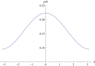 |
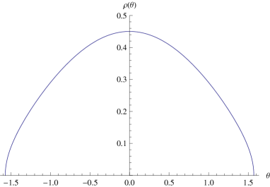 |
It follows from the results just presented that the eigenvalue distributions in the models (7.5) and (7.6) are given by
| (7.8) |
| (7.9) |
To complete the solution to the model we must impose the self consistency conditions on (7.8) and on (7.9). Without loss of generality let us assume that so that . As we have explained above, flat (constant) eigenvalue distributions for both and are always solutions; this solution is stable for and unstable for . It is also easy to check that if the eigenvalue distribution is flat then the same must be true for the eigenvalue distribution, and vica versa. In addition we have four possibilities; each of the and matrix models may be in either the wavy or the clumped phases. We consider each in turn.
7.1.1 wavy, wavy
In this case the self consistency equations are
If and are nonzero, we have a solution only when ; on this solution where (for self-consistency with the assumption that is wavy) but is otherwise arbitrary.
7.1.2 wavy, clumped
In this case the self consistency equations are
These equations admit real solutions only when . The solution is given by
| (7.10) |
Clearly this solution exists only when . The assumption that is wavy is true only when
| (7.11) |
In other words, the solution (7.10) is selfconsistent when
7.1.3 clumped, wavy
It may be verified that there are no solutions of this nature when .
7.1.4 clumped, clumped
In this case the self-consistency equations are
The solution to these equations is given by
| (7.12) |
This solution is consistent with the assumption that is wavy provided that
In other words this solution exists only when
7.1.5 Summary of Solution
In summary, any given temperature (except for the special case ) the toy model has a unique stable saddle point. This saddle point is listed in Table 1. The model starts out in the flat-flat phase, transits to wavy-clumped via a first order phase transition at and then transits to clumped-clumped via a third order phase transition at .
| U | V | |
|---|---|---|
| flat (=0) | flat (=0) | |
| wavy | clumped | |
| clumped | clumped |
7.1.6 Solution obtained by first integrating out
In the first two phases listed in Table 1 above, the eigenvalue distribution for the matrix is ungapped. In these phases the free energy is stationary with respect to a variation of the Fourier modes, , of the eigenvalue distribution of . These two phases may, therefore, simply be studied in an effective matrix model for the matrix , obtained by integrating out classically, using their equations of motion. The part of the action in (7.4) that depends on is given by
On-shell we find , , and (). Integrating out we obtain the following effective matrix model for (note this is accurate only at leading order in )
| (7.13) |
This model was solved in section 6.4 of [20] ( in that paper is our and of that paper should be set to zero). The solution takes the following form. For the eigenvalue distribution is flat, in agreement with Table 1. At the model undergoes a phase transition. The eigenvalue distribution is clumped in the high temperature phase. Using equations 6.11 and 6.18 of [20], it is easily verified that the eigenvalue distribution agrees with that given in (7.9) and (7.10). In particular the value of on this solution is given by (7.10). From the fact that , it follows also that on the solution takes the value presented in (7.10). Consequently the assumption of this section, namely that the eigenvalue distribution is wavy rather than clumped, is self consistent only when the inequality (7.11) is true. When this inequality is violated, our system undergoes a further phase transition (in agreement with Table 1). However this phase transition and the resultant high temperature phase are not accurately captured by the effective model (7.13).
7.2 Effective description of the low and intermediate temperature phase of the full model
We will argue self-consistently below that the qualitative features of the phase diagram of the toy model are also true of the full matrix model (7.2). The full model also undergoes two transitions; the first from uniform-uniform to wavy-clumped and the second from wavy-clumped to clumped-clumped. Exactly as in the previous section, the low and intermediate temperature phases of the full model may be analyzed by integrating out the Fourier modes, , of the holonomy using their equations of motion. Performing this integration (see the previous section for procedure) we obtain the effective matrix model
| (7.14) |
(7.14) has a simple physical interpretation. Note that (7.14) is the free partition function of a gauge theory based on the gauge group . Our effective theory has only adjoint matter, with effective bosonic letter partition function and effective fermionic letter partition function . But this is exactly the partition function for mesonic fields of the sort . In other words (7.14) describes a phase in which the gauge group is completely confined, so that the effective letters and only appear in the combination ; composite letters in the adjoint of . The entire effect of the integration over the holonomy is to effect this complete confinement. The effective description of this phase is in terms of a single gauge group, , and adjoint letters .
This matrix model (7.14) has been studied in detail, in a perturbation expansion in , in section 5.5 of [20]. The qualitative behavior is similar to the toy model studied in the previous section.
7.2.1
In the case that the saddle point is given by
for all . This also implies that
for all . The free energy in this phase vanishes at leading order in . At first subleading order, the partition function (7.2) is obtained by computing the one loop determinant about this saddle point and is given by [20]
| (7.15) |
Note that the result (7.15) diverges when for any . Now is a monotonically increasing function of with and . As for it follows that implies that for all positive . In other words, as is increased from zero (i.e. the temperature of the system is increased from zero) the partition function (7.15) first diverges when , i.e. at . As explained in [20], this divergence has a simple physical interpretation. The effective potential for the mode is proportional to . This potential develops a zero at and is tachyonic for .434343We can see all this directly in the full matrix model (7.2) involving both the and the variables. The potential for the modes and is given by Let and then this potential can be written as is a stable minimum of this potential for . At the potential develops a flat direction that evolves into an unstable direction for . It follows that the trivial solution studied in this subsection is unstable for providing an explanation for the divergence on . At the system undergoes a phase transition to another phase. As we will see below this phase transition is of first order.
7.2.2
The eigenvalue distribution gets increasingly clumped as is increased. Recall that the eigenvalue distribution is determined by the equations
which gives the eigenvalue distribution for as
As is increased this eigenvalue distribution eventually goes negative at for where is a second critical temperature that we will not in generality be able analytically compute in this paper. For the effective action (7.2) is no longer accurate. As in the toy model of the previous section, of course, the physics of this second phase transition is the clumping of the eigenvalue distribution.
7.2.3 The second phase transition at large
When is very large, the second phase transition occurs at a high temperature of order (as we will see below). This results in a key simplification; when the eigenvalue distribution undergoes the phase transition, the eigenvalue distribution is well approximated by a function. In other words for all . Consequently, at leading order in the expansion, the second phase transition is well described by the matrix model
| (7.16) |
When is of order unity, the saddle point to this matrix model is wavy with
so that
| (7.17) |
The leading contribution to free energy computed using this saddle point distribution
| (7.18) |
The first term in the sum vanishes on the saddle point density distribution and we get
| (7.19) |
(7.19) has a simple interpretation. Products of ‘letters’ of the form are singlets under the gauge group U(N), but transform in the adjoint of . The partition function over all bosonic operators is simply given by , while the partition function over all fermionic letters of the same form is given by . (7.19) is precisely the Bose/Fermi exponentiation (multi-particling) of these single meson partition functions. In other words (7.19) is the partition function over a gas of non-interacting mesons of the form . In the limit described in this subsection it follows that the intermediate temperature phase may be thought of as a phase in which the gauge group is completely confined while the gauge group is completely deconfined.
At high temperatures the eigenvalue distribution (7.17) attains its minimum at . This minimum value decreases below zero when
| (7.20) |
As is assumed large in this section, this condition can only be met in the limit that , i.e. in the large limit. At leading order in the large temperature limit (recall ) and
and the eigenvalue distribution (7.17) reduces to
In this approximation the condition (7.20) for the eigenvalue distribution to go negative is given by
| (7.21) |
As it makes no sense for an eigenvalue distribution to be negative, it follows that the matrix undergoes the clumping transition at . Note that is of order , and so is large, as promised at the beginning of this section.
The condition (7.20) gives an expression for the phase transition temperature that may be power series expanded in ((7.21) is the leading term in that expansion). However (7.20) was itself derived under the approximation that the eigenvalue distribution is a delta function. In reality (see below) the eigenvalue distribution has a width of order which is near the phase transition temperature. It is possible to systematically account for the broadening of the eigenvalue distribution (and thereby develop a systematic procedure for computing the phase transition temperature to arbitrary order in ). We demonstrate how this works in Appendix G by computing the first correction to (7.20) resulting from the finite width of the eigenvalue distribution of the matrix .
7.2.4 Effect of interactions on first phase transition
The most general form of effective action in large perturbation theory is
| (7.22) |
Moving to the Fourier basis and integrating out the modes we get an effective adjoint matrix model the matrix
| (7.23) |
where the coefficients can be determined in terms of the coefficients appearing in (7.22). As explained in the [20] the only interaction terms relevant for the phase transition in this adjoint matrix model are
Now we will determine the coefficient of these term in the effective adjoint model in terms of the coefficients appearing in the original matrix model. The relevant part of the original action in Fourier modes is
| (7.24) |
Here and are the Fourier mode of eigenvalue distribution for and matrices respectively and . Also while where is the ’t Hooft coupling. The coefficients and reduces to and respectively in the free theory.The equation of motion for and are
| (7.25) |
Linearizing in and and substituting back the action we get the effective adjoint model (keeping only the terms relevant to phase transition)
| (7.26) |
Now we can again integrate out to get
| (7.27) |
The phase structure described by this effective action was described in [20]. The first order transition of the free theory splits into two phase transitions ; the first of second order (when ) and the next of third order at a higher temperature – if the coefficient of quartic term is negative. However the transition remains a single transition of first order if it is positive; this transition occurs at (see Appendix H). In Appendix H below we demonstrate all this in a somewhat more quantitative fashion by studying interaction in a truncated toy model.
8 Conclusion
In this paper, we proposed the higher spin gauge theories in described by supersymmetric extensions of Vasiliev’s system and appropriate boundary conditions that are dual to a large class of supersymmetric Chern-Simons vector models. The parity violating phase in Vasiliev theory plays the key role in identifying the boundary conditions that preserve or break certain supersymmetries. In particular, our findings are consistent with the following conjecture: starting with the duality between parity invariant Vasiliev theory and the dual free supersymmetric vector model at large , turning on Chern-Simons coupling for the corresponds to turning on the parity violating phase in the bulk, and at the same time induces a change of fermion boundary condition as described in section 5.4.1. We conjectured that the relation , where is the ’t Hooft coupling of the boundary Chern-Simons theory, suggested by two-loop perturbative calculation in the field theory and Giveon-Kutasov duality and ABJ self duality, is exact.
Turning on various scalar potential and scalar-fermion coupling in the Chern-Simons vector model amounts to double trace and triple trace deformations, which are dual to deformation of boundary conditions on spin 0 and spin fields in the bulk theory. Gauging a flavor symmetry of the boundary theory with Chern-Simons amounts to changing the boundary condition on the bulk spin-1 gauge field from the magnetic boundary condition to a electric-magnetic mixed boundary condition. Consideration of supersymmetry breaking by boundary conditions allowed us to identify precise relations between , the Chern-Simons level , and two-point function coefficient in Chern-Simons vector models.
While substantial evidence for the dualities proposed in this paper is provided by the analysis of linear boundary conditions, we have not analyzed in detail the non-linear corrections to the boundary conditions, which are responsible for the triple trace terms needed to preserve supersymmetry. Furthermore, we have not nailed down the bulk theory completely, due to the possible non-constant terms in the function that controls bulk interactions and breaks parity. It seems that etc. cannot be removed merely by field redefinition, and presumably contribute to five and higher point functions at bulk tree level, and yet their presence would not affect the preservation of supersymmetry. This non-uniqueness at higher order in the bulk equation of motion is puzzling, as we know of no counterpart of it in the dual boundary CFT. Perhaps clues to resolving this puzzle can be found by explicit computation of say the contribution of to the five-point function. It is possible that a thorough analysis of the near boundary behavior of solutions to Vasiliev’s equations (via a Graham Fefferman type analysis) could be useful in this regard.
We have also encountered another puzzle that applies to Vasiliev duals of all Chern Simons field theories, not necessarily supersymmetric. Our analysis of the bulk Vasiliev description of the breaking of higher spin symmetry correctly reproduced those double trace terms in the divergence of higher spin currents that involve a scalar field on the RHS. However we were unable to reproduce the terms bilinear in two higher spin currents. The reason for this failure was very general; when acting on a state the higher spin symmetry generators never appear to violate the boundary conditions for any field except the scalar. It would be reassuring to resolve this discrepancy.
The triality between ABJ theory, Vasiliev theory with Chan-Paton factors, and type IIA string theory on suggests a concrete way of embedding Vasiliev theory into string theory. In particular, the Vasiliev theory is controlled by its bulk ’t Hooft coupling . We see clear indication from the dual field theory that at strong , the nonabelian higher spin particles form color neutral bound states, that are single closed string excitations. Vice versa, in the small radius limit and with near critical amount of flat Kalb-Ramond -field on , the type IIA strings should break into multi-particle states of higher spin fields. This picture is further supported by the study of thermal partition function of ABJ theory in the free limit. The dual field theory mechanism for the disintegration of the string is very general, and so should apply more generally to the dual string theory description of any field theory with bifundamental matter, when the rank of one of the gauge groups is taken to be much smaller than the other 444444We thank K. Narayan for discussions on this point. .
In this paper we have computed the thermal phase diagram of ABJ theory in the free limit. This phase diagram has three distinct phases; a low temperature string like phase, an intermediate temperature thermal Vasiliev like phase and a high temperature black hole like phase. It would be very interesting to extend these computations to the interacting theory. Order by order in such computations may be technically feasible nonperturbatively in following the methods employed in [11] and [22].
It has been argued that the vacuum of the ABJ model spontaneously breaks supersymmetry for [31]. Requiring the existence of a supersymmetric vacuum, the maximum value of t’Hooft coupling in a theory with is . As the radius of the dual AdS space in string units is proportional to a positive power of the t’Hooft coupling, it follows that ABJ theories have a weakly curved string description only in the limit . It is interesting that, in the free computations performed above, the new intermediate phase (a free gas of Vasiliev particles) continued to exist all the way upto . If this continues to be the case in the strongly interacting theory, it may be possible to access this new phase at strong coupling via a string worldsheet computation. We find this a fascinating possibility.
More generally, the recasting of ABJ theory as a Vasiliev theory suggests that it would be interesting, purely within field theory, to study ABJ theory in a power expansion in but nonperturbatively in . At this would require a generalization of the results of [8] and [9] to the supersymmetric theory. It may then be possible to systematically correct this solution in a power series in . This would be fascinating to explore.
Perhaps the most surprising recipe in this web of dualities is that the full classical equation of motion of the bulk higher spin gauge theory can be written down explicitly and exactly, thanks to Vasiliev’s construction. One of the outstanding questions is how to derive Vasiliev’s system directly from type IIA string field theory in , or to learn about the structure of the string field equations (in ) from Vasiliev’s equations. As already mentioned, a promising approach is to consider the open-closed string field theory on D6-branes wrapped on , which should directly reduce to Vasiliev theory in the minimal radius limit. It would also be interesting to investigate whether - and in what guise - the huge bulk gauge symmetry of Vasiliev’s description survives in the bulk string sigma model description of the same system. We leave these questions to future investigation.
Acknowledgments.
We would like to thank Xi Dong, Daniel Jafferis, Simone Giombi, Guy Gur-Ari, K. Narayan, Steve Shenker, Sandip Trivedi, Spenta Wadia, Ran Yacoby, and especially Ofer Aharony for useful discussions and comments. We would like to thank Ofer Aharony and Shuichi Yokoyama for help comments on preliminary draft of this paper. XY would like to thank Tata Institute of Fundamental Research, Aspen Center for Physics, Harish-Chandra Research Institute, Simons Center for Geometry and Physics, Stanford University, California Institute of Technology, Weizmann Institute, Kavli Institute for Theoretical Physics, and Lebedev Institute for hospitality during the course of this work. CC would like to thank National Taiwan University and National Tsing Hua University for hospitality during the course of this work. SM would like to thank Harish Chandra research institute and Cargese summer school for hospitality while this work was in progress. The work of CC and XY are supported in part by the Fundamental Laws Initiative Fund at Harvard University, and by NSF Award PHY-0847457. The work of SM is supported in part by Swarnjayanti fellowship. SM and TS would like to acknowledge our debt to the people of India for their generous and steady support to research in the basic sciences. \appendixpage\addappheadtotocAppendix A Details and explanations related to section 2
A.1 Star product conventions and identities
It follows from the definition of the star product that
| (A.1) |
Identical equations (with obvious modifications) apply to the bar variables. Spinor indices are lowered using the tensor as follows
| (A.2) |
Note that for an arbitrary function we have
| (A.3) |
Using (A.3) we the following (anti)commutator
| (A.4) |
It follows from (A.1) that
| (A.5) |
Similar expression(with obvious modifications) are true for (anti)commutators with and . Substituting into (A.3) and using , one obtains
| (A.6) |
In a similar manner we find
On the other hand clearly commutes with and . The second line of (LABEL:kprop) follows immediately from these observations.
The first line of (LABEL:kprop) is also easily verified.
A.2 Formulas relating to operation
We now demonstrate that
if and are each oneforms.
| (A.8) |
A.3 Different Projections on Vasiliev’s Master Field
One natural projection one might impose on the Vasiliev master field is to restrict to real fields where reality is defined by
| (A.9) |
This projection preserves the reality of the field strength (i.e. is real if is). As we will see below, however, the projection (A.9) does not have a natural extension to the supersymmetric Vasiliev theory, and is not the one we will adopt in this paper.
The second ‘natural’ projection on Vasiliev’s master fields is given by
| (A.10) |
Note that the various components of transform homogeneously under this projection
| (A.11) |
(the signs in (A.10) were chosen to ensure that all the quantities in (A.11) transform homogeneously). Note also that
| (A.12) |
(we have used ).
A.4 More about Vasiliev’s equations
Expanded in components the first equation in (LABEL:veqns) reads
| (A.14) | ||||
The second equation reads
| (A.15) | ||||
We will now demonstrate that the second equation in (LABEL:veqns) follows from the first (i.e. that (LABEL:veqnsc) follows from (LABEL:veqnsb)). Using (2.21) and the first of (LABEL:veqns) we conclude that
| (A.16) |
The components of (A.16) proportional to yield,
| (A.17) |
Multiplying this equation by from the right and using we find the first of (LABEL:veqnsc).
The components of (A.16) proportional to yield
| (A.18) |
Multiplying this equation by from the right and using (the second step uses the truncation condition (2.11) on ) we once again find the first of (LABEL:veqnsc).
The term in (A.16) proportional to and may be processed as follows. Let
| (A.19) |
where is proportional to and is proportional to . The part of (A.16) proportional to yields
| (A.20) |
Multiplying this equation with from the right and using we find
| (A.21) |
A.5 Onshell (Anti) Commutation of components of Vasiliev’s Master Field
In this subsection we list some useful commutation and anticommutation relations between the adjoint fields , , and . The relations we list can be derived almost immediately from Vasiliev’s equations; we list them for ready reference
| (A.24) |
The derivation of these equations is straightforward. The first equation follows upon expanding the commutator and noting that (this follows from (2.11) together with the obvious fact that and commute). The second equation in (A.24) follows upon inserting the decomposition (A.19) into the third equation in (LABEL:veqnsb). The third and fourth equations in (A.24)are simply (A.20) and (A.22) rewritten.
The fifth equation in (A.24) may be derived from the third equation as follows
| (A.25) |
In the third line of (A.25) we have used the truncation condition (2.11)
The sixth equation in (A.24) is derived in a manner very similar to the fifth equation.
A.6 Canonical form of in Vasiliev’s equations
In this subsection we demonstrate that we can use the change of variables for some odd real function together with multiplication by an invertible holomorphic even function to put any function in the form (2.30), atleast provided that the function admits a power series expansion about and that .
An arbitrary function may be decomposed into its even and odd parts
If in invertible then the freedom of multiplication with an even complex function may be used to put in the form
where . Clearly is an odd function that admits a power series expansion. Atleast in the sense of a formal power series expansion of all functions, it is easy to convince oneself that any such function may be written in the form where is an a real odd function and is a real even function. We may now use the freedom of variable redefinitions to work with the variable instead of . This redefinition preserves the even nature of and casts in the form (2.30).
A.7 Conventions for spinors
Euclidean matrices may be chosen as
| (A.26) |
where and
| (A.27) |
(where and are the usual Pauli matrices). In the text below we will often refer to the fourth component of as ; in other words
(we adopt this cumbersome notation to provide easy passage to different conventions). The chirality matrix is given by
| (A.28) |
matrices act on the spinors
whereas the row spinors that multiply from the left have the index structure
As a consequence we assign the index structure and It is easy to check that
| (A.29) |
where
| (A.30) |
Clearly the index structure above is and . Spinor indices are raised and lowered according to the conventions
The product of a chiral spinor and an antichiral spinor is a vector. By convention we define the associated vector as
| (A.31) |
The product of a chiral spinor with itself is a self dual antisymmetric 2 tensor which we take to be
| (A.32) |
Similarly the product of an antichiral spinor with itself is an antiselfdual 2 tensor which we take to be
| (A.33) |
A.8 solution
In this appendix we will show that
| (A.34) |
with the values for the vielbein and spin connection, satisfies the Vasiliev equation
| (A.35) |
Substituting (A.34) in (A.35) and collecting terms quadratic in and we get
| (A.36) |
Let us consider the Vasiliev gauge transformations generated by
Under these the vielbein and spin connection changes by
| (A.37) |
Notice that these are just the rotation of the vielbeins in the tangent space. The two homogeneous terms in are just the rotation by under and of that acts on the tangent space. As expected under such rotation the spin connection transforms inhomogeneously. Substituting (A.37) in (A.36) it is easily verified that (A.36) transforms homogeneously.
In fact the first equation in (A.36) is just the torsion free condition while the second and third equation expresses the selfdual and anti-selfdual part of curvature two form in term of vielbeins. Substituting the values of vielbeins and spin connection (LABEL:ewsol) one can easily check that (A.36) are satisfied.
Converting (A.36) from bispinor notation to vector notation using the following conversion
| (A.38) |
we get
| (A.39) |
A.9 Exploration of various boundary conditions for scalars in the non abelian theory
The same theory in with boundary condition on the -singlet bulk scalar is dual to the critical point of the vector model with flavors and the double trace deformation by . Alternatively, this critical point may be defined by introducing a Lagrangian multiplier and adding the term
| (A.40) |
to the Lagrangian of the vector model.454545The critical point can be conveniently defined using dimensional regularization. As in the case of the critical vector model, higher spin symmetry is broken by effects. Note that the part of the spin-2 current is also broken by effects, i.e. there are no interacting colored massless gravitons, as expected. To see this explicitly from the boundary CFT, let us consider the spin-2 current
| (A.41) |
Using the classical equation of motion
| (A.42) |
we have
| (A.43) |
While the -singlet part of , being the stress-energy tensor, is conserved ( is set to zero by -equation of motion), the non-singlet part of is not conserved, and acquires an anomalous dimension of order at the leading nontrivial order in the expansion. In the bulk, the colored gravitons become massive, and their longitudinal components are supplied by the bound state of the singlet scalar and a colored spin-1 field.
One could also consider the theory in with boundary condition on all bulk scalars, that is, on both the singlet and adjoint of the bulk gauge group. The dual CFT is the critical point defined by turning on the double trace deformation and flow to the IR, or by introducing the Lagrangian multiplier , and the term
| (A.44) |
in the CFT Lagrangian. Now the classical equations of motion
| (A.45) |
imply the divergence of the colored spin-2 currents
| (A.46) |
Once again, the non-singlet spin-2 current is no longer conserved. In this case, the colored gravitons in the bulk are massive because their longitudinal component are supplied by the two-particle state of colored scalar and spin-1 fields.
Appendix B Supersymmetry transformations on bulk fields of spin , , and
We begin by rewriting the magnetic boundary condition on the spin-1 bulk fields in the supersymmetric Vasiliev theory. With the magnetic boundary condition, the vector gauge fields are dual to ungauged “R-symmetry” currents of boundary CFT that rotate the bosonic and fermionic flavors separately. Supersymmetrizing Chern-Simons coupling will generally break this flavor symmetry to a subgroup. We will see this as the violation of magnetic boundary condition by the supersymmetry variation of the bulk spin-1 fields. If we do not gauge the flavor symmetries of the Chern-Simons vector model, then all bulk vector fields should be assigned the magnetic boundary condition. We will see later that in this case only up to supersymmetry can be preserved, whereas by relaxing the magnetic boundary condition on some of the bulk vector fields, it will be possible to preserve or supersymmetry.
In terms of Vasiliev’s master field which contains the field strength, the general electric-magnetic boundary condition may be expressed as
| (B.1) |
where and its complex conjugate are functions of , and are constrained by the linear relation
| (B.2) |
With this choice of boundary condition, the boundary to bulk propagator for the spin-1 components of the master field is given by the standard one,
| (B.3) | ||||
It indeed obeys (B.2), with and given by
| (B.4) | ||||
and
| (B.5) |
In the next four subsections, we give the explicit formulae for the supersymmetry variation (i.e. spin gauge transformation of Vasiliev’s system) of bulk fields of spin , sourced by boundary currents of spin .
B.1 : spin 1 spin
Let us start with the master field sourced by a spin-1 boundary current at , i.e. the spin-1 boundary to bulk propagator , and consider its variation under supersymmetry, which is generated by of degree one in :
| (B.6) | ||||
Carrying out the products explicitly, we find
| (B.7) | ||||
and
| (B.8) | ||||
Note that the commutators and anti-commutators in above formula are due to the -dependence only, and do not involve product. contains supersymmetry variation of fields of spin and . We will focus on the variation spin fields, since they can be subject to a family of different boundary conditions, corresponding to turning on fermionic double trace deformations (i.e. ) in the boundary CFT. So we restrict to terms linear in ,
| (B.9) | ||||
where in the second line we kept the leading terms, of order , in the limit.
B.2 : spin spin
The general conformally invariant boundary condition on spin fermions, in terms of Vasiliev’s master field, takes the form
| (B.10) |
Here and its complex conjugate are chiral and anti-chiral spinors that are odd functions of the Grassmannian variables . They are further constrained by the linear relation
| (B.11) |
is generally a linear operator that acts on the vector space spanned by odd monomials in the ’s, i.e. it assigns phase angles to fermions in the bulk -symmetry multiplet. A choice of the spin- fermion boundary condition is equivalent to a choice of the “phase angle” operator .
The fermion boundary to bulk propagator that satisfies the above boundary condition is:
| (B.12) | ||||
Here the linear operator is understood to act on only, the latter being an odd function of ’s.
Next, we make super transformation on the fermion boundary to bulk propagator. The supersymmetry transformation reads
| (B.13) | ||||
where , is an odd supersymmetry parameter multiplied by an odd function of the ’s. in particular anti-commutes with all ’s, and therefore anti-commutes with which involves an odd number of ’s.
Carrying out the algebra, we have
| (B.14) | ||||
and
| (B.15) | ||||
The supersymmetry variation of the spin-1 field strengths are extracted from terms in , namely
| (B.16) | ||||
In the second line, we have taken the small limit and kept the leading terms, of order .
B.3 : spin spin
The supersymmetry variation of the scalar field due to a spin- fermionic boundary source is extracted from of the previous subsection, restricted to :
| (B.17) | ||||
In the last two lines, as a linear operator is understood to act on only (and not on ).
B.4 : spin spin
The general conformally invariant linear boundary condition on the bulk scalars may be expressed as
| (B.18) |
in the limit . Here are real and even function in , and are subject to a set of linear relations that eliminate half of their degrees of freedom. The phase is generally a linear operator acting on the space spanned by even monomials in the ’s (analogously to in the fermion boundary condition). We will determine our choice of and the linear constraints on later.
The boundary-to-bulk propagator for the scalar components of the master field, subject to the above boundary condition, is now written as
| (B.19) |
where
| (B.20) |
A straightforward calculation gives the supersymmetry variation of the spin- fermion due to a scalar boundary source at ,
| (B.21) | ||||
We have taken the small limit, and kept terms of order . Again, in the last two lines as a linear operator should be understood as acting on only and not on .
Appendix C The bulk dual of double trace deformations and Chern Simons Gauging
C.1 Alternate and Regular boundary conditions for scalars in
In this section we review the AdS/CFT implementation alternate and regular boundary conditions for scalars, in the presence of multitrace deformations. The material reviewed here is well known (see e.g. [17, 32, 33, 34, 35, 18] - we most closely follow the approach of the paper [33]); our brief review focuses on aspects we will have occasion to use in the main text of our paper.
C.1.1 Multi-trace deformations in large field theories
In this brief subsection we will address the following question: how is the generating function of correlators of a large field theory modified by the addition of a multi-trace deformation to the action of the theory?
Consider any large field theory whose single trace operators are denoted by . Let denote the generating function of correlators464646More precisely this equation should have read (C.1) However for ease of readability, in all the formal discussions of this section we will use compact notation in which we suppress the position dependence of operators and fields, and do not explicitly indicate integration.
| (C.2) |
Note that is of order in a matrix type large theory, while it is of order in a vector type large theory. For formal purposed below we will find it useful to Legendre transform to define an effective action for the operators
| (C.3) |
is a function only of (and not of ) in the following sense. The RHS of (C.3) is viewed as an action for the dynamical variable . The equation of motion for follows from varying this action and is
| (C.4) |
The RHS of (C.3) is evaluated with the onshell value of .
plays the role of the effective action for the trace operators . In the large limit the dynamics of the operators is generated by the classical dynamics of the action .
Of course may equally be thought of as the Legendre transform of
| (C.5) |
where is the function of obtained by solving the equation of motion
| (C.6) |
Now let us suppose that the action of the original large field theory is deformed by the addition of a multitrace term where is an arbitrary function of . The effective action for this deformed theory is simply given by
| (C.7) |
The generating function of correlators of the deformed theory is once again given by the Legendre transform (C.5) with replaced by .
C.1.2 Bulk dual to multi trace deformations in regular and alternate quantization
Consider a real scalar field propagating in according to the action
| (C.8) |
It is well known that these scalars admit two distinct conformally invariant boundary conditions - sometimes referred to as alternate and standard quantization - in the mass range . In this subsection we will review the very well known rules for the computation of correlation functions for scalars with alternate and standard boundary conditions.
The action (C.8) is ambiguous as it generically receives divergent contributions from the boundary, as we now explain. We use coordinates so that the metric of AdS space is given by (2.33). Near the general solution to the equation motion from (C.8) takes the form
| (C.9) |
where is the positive root of the equation . Let us cut of the action (C.8) at a small value, of the coordinate . Onshell (C.8) evaluates to
| (C.10) |
where the integral is evaluated over the boundary surface . It is easily verified that the action has a divergence proportional to when evaluated on the generic solution (C.9). To cure this divergence we supplement (C.8) with a diffeomorphically invariant boundary action for the dimensional boundary field
| (C.11) |
where, once again, the integral is taken over the boundary surface and is the induced metric on this boundary. It is easily verified that
| (C.12) |
Regularity in the interior of relates to . The relationship is clearly linear and so takes the form
| (C.13) |
In the rest of this subsection we use abbreviated notation so that (C.14) is written as and (C.13) is written as . It follows that the onshell action is given by
| (C.14) |
In the case of alternate quantization the boundary action (C.14), thought of as a functional of the dynamical field , is identified with the single trace effective action defined in (C.3). The generator of correlators of this theory is obtained by coupling to a source :
| (C.15) |
The resulting equation of motion for yields
| (C.16) |
Integrating out we find the action
It follows that the two point function of the dual operator is . It also follows from (C.16) that
in particular vanishes wherever vanishes. Consequently, alternate quantization is associated with the boundary condition .
The multi trace deformation of the dual theory is implemented, in alternate quantization, by adding the term to the boundary effective action (C.14), in perfect imitation of (C.7). Correlation functions of the deformed theory are obtained by the Legendre transform of this augmented boundary action. The resultant equation of motion is yields the bulk boundary conditions
In the case of regular quantization we supplement the action (C.14) with an additional degree of freedom so that the full boundary action takes the form
| (C.17) |
The dynamical field is then integrated out using its equation of motion
| (C.18) |
On shell, therefore . The resultant action
| (C.19) |
as a function of is identified with in (C.3). The generator of correlators of the theory is obtained by coupling to a source
and then integrating this field out according to its equations of motion. This allows us, in particular, to identify the two point function of the dual theory with . Note also that the resultant equation of motion, implies
so that vanishes wherever vanishes. In other words standard quantization is associated with the boundary condition . The multitrace deformation of the dual theory is implemented, in standard quantization, by adding to the action (C.19). The resultant boundary condition is
C.1.3 Marginal multitrace deformation with two scalar field in opposite quantization
Consider two scalar fields in , and , with quantized with alternate quantization and with regular quantization. In the compact notation defined in earlier subsection, the generating function of correlation function of the dual field theory deformed by double trace operator is
| (C.20) |
The action is linear in ; the equation of motion for this field immediately yields
| (C.21) |
Using (C.21) to eliminate in favor of , simplifies to a function of . The resultant equation of motion yields
| (C.22) |
Using and , (C.22) may be rewritten as
| (C.23) |
Upon setting , (C.21) and (C.23) express the boundary conditions of the trace deformed model. These boundary conditions may, most succinctly be expressed as follows. Let us define new ’rotated’ bulk fields
Note that the rotated fields have same bulk action as the original fields. The boundary conditions (C.21) and (C.23) reduce to
In summary dual to the the double trace deformed field theory has the same action as well as boundary conditions for and as the dual to the undeformed theory had for and . Despite this fact, the double trace deformed theory is not field redefinition equivalent to the original theory. This can be seen in many ways. Most simply, the full action (C.20) does not have a simple rotational invariance, and does not take a simple form when reexpressed in terms of and . This lack of equivalence also shows itself up in the generator of two point functions of the operators dual to and . This generating function is obtained by plugging (C.21) and (C.22) into (C.20); we find
| (C.24) |
The fact that does not disappear from (C.24) demonstrates the lack of equivalence of the trace deformed model from the trace undeformed model (). Note in particular that the double trace deformed theory has a contact cross two point function
which is absent in the trace undeformed theory. On the other hand the direct correlators and have the same spacetime structure in the deformed and undeformed theories, but have different normalizations.
C.2 Gauging a symmetry
Let us begin with a three dimensional CFT with a global symmetry, generated by the current , where is the three-dimensional vector index. This theory will be referred to as CFT∞, as opposed to the theory obtained by gauging the with Chern-Simons gauge field at level , which we refer to as CFTk. Suppose CFT∞ is dual to a weakly coupled gravity theory in . The global current of the boundary CFT is dual to a gauge field in the bulk. The two-derivative part of the bulk action for the gauge field is
| (C.25) |
Working in the radial gauge , we have
| (C.26) |
Consider the linearized, i.e. free, equation of motion
| (C.27) |
together with the constraint
| (C.28) |
Near the boundary, a solution to the equation of motion has two possible asymptotic behaviors, , or . Equivalently, they can be expressed in gauge invariant form as the magnetic boundary condition
| (C.29) |
and the electric boundary condition
| (C.30) |
respectively. With the magnetic boundary condition, is dual to a global current in the boundary CFT, i.e. CFT∞. The family of CFTk, on the other hand, is dual to the same bulk theory with the mixed boundary condition (still conformally invariant)
| (C.31) |
Here is a constant. It will be determined in terms of the two-point function of the current .
Let us now solve the bulk Green’s function with the mixed boundary condition. The bulk linearized equation of motion with a point source at , after a Fourier transformation in the boundary coordinates , is
| (C.32) |
Due to the constraint (C.28), the source is restricted by . The boundary condition is
| (C.33) |
Without loss of generality, let us consider the case , and assume . The Green equation is now written as
| (C.34) | ||||
and the boundary condition as
| (C.35) |
The -independent part of can be gauged away. We may then take the solution
| (C.36) | ||||
where and obey
| (C.37) | ||||
The solutions are
| (C.38) |
The nontrivial components of Green’s function are thus given by
| (C.39) | ||||
In particular, we find the change of the bulk Green’s function due to the changing of the boundary condition,
| (C.40) |
The boundary to bulk propagator for can be obtained by taking limit on , giving
| (C.41) | ||||
We observe that factorizes into the product of two boundary to bulk propagators, and , multiplied by
| (C.42) |
This is reminiscent of the change of scalar propagator due to boundary conditions [50, 7]. So far we worked in the special case . Restoring rotational invariance, (C.42) is replaced by
| (C.43) | ||||
In the boundary CFT, the change of boundary condition amounts to coupling the current to a boundary gauge field at Chern-Simons level . is proportional to the two-point function of in the Lorentz gauge . Namely,
| (C.44) |
where is the overall normalization factor in the two-point function of the current ,
| (C.45) |
Our convention is such that in the free theory counts the total number of complex scalars and fermions. Note that here we are normalizing the current coupled to the Chern-Simons gauge field according to the convention for nonabelian gauge group generators, for generators , in the fundamental representation. This is also the normalization convention we use to define the Chern-Simons level (which differs by a factor of 2 from the natural convention for gauge group).
To see this, note that the inverse of the matrix in (C.42), restricted to directions transverse to , is
| (C.46) |
After restoring rotational invariance, this is
| (C.47) |
which for precisely matches times the kinetic term of the Chern-Simons gauge field plus the contribution to the self energy of from .
Appendix D Supersymmetric Chern-Simons vector models at large
In this appendix, we review the Lagrangian of Chern-Simons vector models with various numbers of supersymmetries and/or superpotentials. The scalar potentials and scalar-fermion coupling resulting from the coupling to auxiliary fields in the Chern-Simons gauge multiplet and superpotentials can be expressed in terms of bosonic or fermionic singlets under the Chern-Simons gauge group as double trace or triple trace terms. These can be matched with the change of boundary conditions in the holographically dual Vasiliev theories in , described in section 4.
D.1 theory with chiral multiplets
The action of the pure Chern-Simons theory in Lorentzian signature is
| (D.1) |
where and are fermionic and bosonic auxiliary fields. The chiral multiplets in the fundamental representation couple to the gauge multiplet through the action
| (D.2) |
We will focus on the matter coupling
| (D.3) |
Integrating out the auxiliary fields, we obtain the scalar potential and scalar-fermion coupling,
| (D.4) |
For the purpose of comparing with vector models of other numbers of supersymmetries, it is useful to consider the case. Let us define bosonic and fermionic gauge invariant bilinears in the matter fields,
| (D.5) |
where . The non-supersymmetric theory with two flavors and without matter self-interaction would have had flavor symmetry acting on the bosons and fermions separately. With respect to this symmetry, , and are in the representation , and respectively. Expressed in terms of the bosonic and fermionic singlets, can be written as
| (D.6) |
Note that the terms is invariant under , whereas the term and the scalar potential explicitly break to the diagonal flavor .
Indeed, the boundary conditions of the conjectured holographic dual described in section 4.3.1 are such that the fermionic boundary condition (characterized by ) is invariant under the that rotates the four Grassmannian variables of supersymmetric Vasiliev theory, while the scalar boundary condition only preserve an subgroup.
D.2 theory with chiral multiplets
The theory in the previous section admits a one-parameter family of exactly marginal deformations that preserves supersymmetry. The matter coupling of this theory is given by
| (D.7) | ||||
where is a real deformation parameter. The theory is given by .
D.3 The theory with chiral multiplets and chiral multiplets
Now we turn to the Chern-Simons vector model with an equal number of fundamental and anti-fundamental chiral multiplets. This model differs from the theory with fundamental chiral multiplets through the scalar-fermion coupling and scalar potential only. The part of the Lagrangian that couples matter fields to the auxiliary fields in the gauge multiplet is given by
| (D.8) | ||||
Integrating out the auxiliary fields, we obtain
| (D.9) | ||||
D.4 The theory with hypermultiplets
The Chern-Simons vector model with hypermultiplets can be obtained from the theory described in the previous subsection by adding the superpotential [51, 28]
| (D.10) |
where is an auxiliary chiral superfield. Integrating out , we obtain a quartic superpotential
| (D.11) |
After integrating over the superspace, we obtain
| (D.12) |
Integrating out the auxiliary fields , the -term potential is
| (D.13) | ||||
The total potential is given by the -term plus -term potentials:
| (D.14) |
To make the R-symmetry manifest, we rewrite the potential in terms of the doublets:
| (D.15) |
The -term and -term potentials are
| (D.16) | ||||
and
| (D.17) | ||||
We have also suppressed the flavor indices. The total potential can be written in a R-symmetry manifest way:
| (D.18) |
where contains the double trace operator of the form ,
| (D.19) |
is the scalar potential in the form of a triple trace term,
| (D.20) |
is the double trace term of the form ,
| (D.21) |
where are defined as
| (D.22) |
and are antisymmetric tensors with .
For reference in main text we will record the double trace part of the potential in vector notation. Let us define
| (D.23) |
where
Here are Pauli sigma matrices. The a,b indices runs over 1,2,3,0. A,B runs over 1,2. and transform under the as vectors of which under transform as singlet(a=0) and a vector(a=1,2,3) while transform as doublets of .
| (D.24) |
D.5 A family of theories with a chiral multiplet and a chiral multiplet
If we deformed the superpotential in the above subsection as
| (D.25) |
the supersymmetry is broken to . In this case, the potential is
| (D.26) |
where contains the double trace operator of the form ,
| (D.27) |
is the scalar potential in the form of a triple trace term,
| (D.28) | ||||
is the double trace term of the form ,
| (D.29) | ||||
D.6 The theory with one hypermultiplet
As shown by [29], Chern-Simons vector model with hypermultiplets can be deformed to an quiver type Chern-Simons matter theory by gauging (a subgroup of) the flavor group with another Chern-Simons gauge multiplet, at the opposite level . Here we will focus on the case where the entire is gauged, so that the resulting theory has Chern-Simons gauge group and a single bifundamental hypermultiplet. This theory will still be referred to as a vector model, as we will be thinking of the ’t Hooft limit of taking large and kept finite. As we have seen, turning on the finite Chern-Simons level for the flavor group amounts to simply changing the boundary condition on the vector gauge fields in the bulk Vasiliev theory.
The part of the Lagrangian that couples matter fields to the auxiliary fields in the gauge multiplet is given by
| (D.30) | ||||
where we suppressed the both and indices. Integrating out the auxiliary fields, we obtain the potential:
| (D.31) | ||||
The complex scalar and the fermion transform as and under the R-symmetry. The potential (D.31) is manifestly invariant under the R-symmetry.
For reference to main text we now record the double trace part of this potential in vector notation. Using the definitions (D.23), the (scalar singlet)2 part() and (fermion singlet)2 part() are given by
| (D.32) |
D.7 theories with one hypermultiplet
The theory in the previous section sits in a discrete one parameter family of theories with one hypermultiplet. The potential can be written in an R-symmetry manifest way:
| (D.33) |
where contains the double trace operator of the form ,
| (D.34) |
is the scalar potential in the form of triple trace term. is the double trace term of the form ,
| (D.35) | ||||
In the notation defined in (D.23) and becomes
| (D.36) |
D.8 The theory
The above theory can be generalized to a quiver theory with hypermultiplets by starting with the Chern-Simons vector model with hypermultiplets and only gauging the subgroup, of the flavor group, at level with another Chern-Simons gauge multiplet. The resulting theory has flavor symmetry. For generic value of , the theory has sypersymmetry, but for , the theory exhibits sypersymmetry, respectively. Let us focus on the case. The part of the Lagrangian that couples matter fields to the auxiliary fields in the gauge multiplet is given by
| (D.37) | ||||
where are the indices. There is also an superpotential
| (D.38) |
After integrating over the superspace, we obtain
| (D.39) |
After integrating out all the auxiliary fields, the resulting potential can be written in a R-symmetry manifest way:
| (D.40) |
where contains the double trace operator of the form ,
| (D.41) | ||||
where we have rewrite the potential in terms of the doublets (D.15), and are the spinor indices. is the scalar potential in the form of triple trace term. is the double trace term of the form ,
| (D.42) |
where .
D.9 theories with two hypermultiplets
The theory in the previous section sits in a discrete one parameter family of theories with two hypermultiplets. The superpotential of these theories are
| (D.43) |
where are the flavor indices. The potential can be written in an R-symmetry and flavor symmetry manifest way:
| (D.44) |
where contains the double trace operator of the form ,
| (D.45) |
where we have rewrite the potential in terms of the doublets (D.15), and are the spinor indices. is the scalar potential in the form of triple trace term. is the double trace term of the form ,
| (D.46) | ||||
Now we record the double trace parts of the potential in vector notation of symmetry. Let us define
| (D.47) |
Here both set of indices I,J as well i,j run over 1,2,3,0. I,J are the vector indices of while i,j are vector indices of . The 0 component corresponds to the singlet while 1,2,3 represents the vector part. In this notation the double trace potential part of the becomes
| (D.48) |
The double potentials for theory is obtained from (D.48) on setting .
Appendix E Argument for a Fermionic double trace shift
In this Appendix compare the boundary conditions and Lagrangian for the fixed line of theories to argue for the effective shift of fermionic boundary conditions induced by the Chern Simons term.
Let us use the notation and for field theory single trace operators. We know that a double trace deformation proportional to is dual to fermion boundary condition (4.8) with . On the other hand the double trace deformation is dual to the fermion boundary condition with . Now in the zero potential theory () the relevant terms in (D.7) are
while . At the point, on the other hand, the fermion double trace term is
while . Subtracting these two data points we conclude that the double trace deformation by
is dual to a boundary condition deformation with . By symmetry it must also be that the double trace deformation by
is dual to a boundary condition deformation with . Adding these together, it follows that a double trace deformation by
is dual to the boundary condition deformation with . But the theory with this boundary condition has a double trace potential equal only to
For consistency, it must be that the Chern Simons interaction itself induces a change in fermion boundary conditions equal to that one would have obtained from a double trace deformation
| (E.1) |
Appendix F Two-point functions in free field theory
Consider the action for free theory of a boson and a fermion in the fundamental representation, in flat 3 dimensional euclidean space
| (F.1) |
where the in indices are suppressed and will continue to be in what follows. The Green’s functions for the scalar and fermions are given by
| (F.2) |
Let us define the ’Single Trace’ operators
| (F.3) |
In the free theory
| (F.4) |
Appendix G Corrections at large
The expression for presented in (7.20) receives corrections in a power series expansion in . In this Appendix we compute the first correction to the expression for the second phase transition temperature presented in (7.20) at small .
(7.20) receives corrections once we take into account the fact that the eigenvalue distribution is not quite a delta function in the neighborhood of the phase transition. To compute the leading correction to eigenvalue distribution of V-matrices we substitute
for odd , and
for even (see (7.17)). It follows that the effective matrix integral for V-matrices is given by
| (G.1) |
The saddle point equation for this model is
| (G.2) |
To leading order in the V-eigenvalues are clumped into a delta function around zero. To first subleading order we expect that the eigenvalues will spread but only in a small region around zero and vanishes outside. Since all the eigenvalues are small the above saddle point equation reduces to hermitian wigner model
| (G.3) |
The solution to the above Wigner model is
| (G.4) |
Using this one can compute
| (G.5) |
where is Bessel function. Substituting these into (7.2) and using saddle point approximation one gets the corrected eigenvalue distribution for U-matrices to be
| (G.6) |
At leading order at high temperatures we substitute . The leading correction to the eigenvalue distribution (from the finite width of the eigenvalue distribution) is given by
| (G.7) |
where is the Riemann zeta function with = 1.202.
The shift in the eigenvalue distribution evaluated at is given, to leading order in large , by
This results is a shift of the phase transition temperature (about the result (7.20) at leading order at large )
Thus the finite width of the eigenvalue distribution gives rise to a fractional correction of order second phase transition temperature.
Appendix H Truncated toy matrix model including interaction effects
In this Appendix we study the toy model
| (H.1) |
in a neighborhood of , with and taken to be small.
The saddle point equations for the for U and V eigenvalues are
| (H.2) |
These equations are of the Gross-Witten-Wadia form with the Gross-Witten-Wadia coupling dependent on the and themselves. We now search for self consistent solutions to these equations.
H.1 flat, flat
we see that the = = 0 for all n, is always a solutions.
H.1.1 flat, wavy or vice-versa
Substituting either or to zero we see that the other one is necessarily zero. Thus flat-wavy or wavy-flat is not a solution.
H.2 wavy, wavy:
In this case we will have
| (H.3) |
These equations may be used solve for and ; without loss of generality we may choose and each to be real so that and . We find
| (H.4) |
When is positive this solution only makes sense for . On the other hand when is negative, the solution only makes sense for .
Consistency of the solution(positivity of eigenvalue density distribution) further requires
| (H.5) |
As the first of these two conditions is stronger. When is positive this condition amounts to the requirement that
When is negative this condition amounts to the requirement that
In summary, when is positive the wavy-wavy solution exists for
At the lower end of this range the eigenvalue distribution is on the border of being gapped, while at the upper end of this range the and eigenvalue distributions are both flat.
When is negative, on the other hand, the wavy-wavy solution exists for
At the lower end of this range the eigenvalue distribution becomes flat, while at the upper end of this range the eigenvalue distribution is at the edge of being gapped.
H.3 wavy, clumped
In this case we have
| (H.6) |
We may solve for in terms of and then obtain an equation for as follows
| (H.7) |
Again consistency of solution requires
| (H.8) |
The second condition is satisfied if and only if
| (H.9) |
When this inequality is saturated, the eigenvalue distribution is on the border between wavy and clumped. The first condition is saturated at a higher temperature when the eigenvalue distribution first begins to clump (i.e. near the second phase transition of the free model). As the quartic interaction are not particularly important for this transition, we do not study this transition in detail.
It is possible to verify that solutions of the clumped wavy form do not exist. As mentioned above, clumped-clumped solutions do exist, but the quartic interaction terms do not play an important role in determining their properties, and we do not consider them further here.
H.4 Summary
The quartic interaction terms of this subsection qualitatively modify the nature of the first phase transition of the free theory.
When is positive the flat-flat configuration is the only solution to the saddle point equations when . At this temperature two new solutions are nucleated. The first is a wavy wavy solution is a local maximum and so is unstable throughout the range of its existence. The second is a wavy-clumped solution and is locally solution. At the free energy of the wavy-clumped solution decrease below that of the flat-flat solution and the system undergoes a first order phase transition. At the higher temperature the wavy-wavy solution merges with the flat flat solution and ceases to exist thereafter. At higher temperatures the flat-flat solution is unstable and the wavy-clumped solution is the unique stable saddle point. At still higher temperatures this saddle point undergoes a 3rd order phase transition to the clumped-clumped saddle.
When is negative the flat-flat configuration is the only solution to the saddle point equations when . At this temperature the flat-flat saddle goes unstable, but a wavy-wavy solution is nucleated, and is stable at higher temperatures. The system undergoes a second order phase transition (from the flat-flat saddle to the wavy-wavy saddle) at . At ( recall this is a higher temperature than because is negative) the wavy-wavy saddle turns into a wavy-clumped saddle through a third order phase transition. At still higher temperatures the wavy-clumped saddle point undergoes a 3rd order phase transition to the clumped-clumped saddle.
References
- [1] I. Klebanov and A. Polyakov, AdS dual of the critical O(N) vector model, Phys.Lett. B550 (2002) 213–219 [hep-th/0210114].
- [2] E. Sezgin and P. Sundell, Massless higher spins and holography, Nucl.Phys. B644 (2002) 303–370 [hep-th/0205131].
- [3] E. Sezgin and P. Sundell, Holography in 4D (super) higher spin theories and a test via cubic scalar couplings, JHEP 07 (2005) 044 [hep-th/0305040].
- [4] S. Giombi and X. Yin, Higher Spin Gauge Theory and Holography: The Three-Point Functions, JHEP 1009 (2010) 115 [0912.3462].
- [5] S. Giombi and X. Yin, Higher Spins in AdS and Twistorial Holography, JHEP 1104 (2011) 086 [1004.3736].
- [6] S. Giombi, S. Prakash and X. Yin, A Note on CFT Correlators in Three Dimensions, 1104.4317.
- [7] S. Giombi and X. Yin, On Higher Spin Gauge Theory and the Critical O(N) Model, 1105.4011.
- [8] J. Maldacena and A. Zhiboedov, Constraining Conformal Field Theories with A Higher Spin Symmetry, 1112.1016.
- [9] J. Maldacena and A. Zhiboedov, Constraining conformal field theories with a slightly broken higher spin symmetry, 1204.3882.
- [10] O. Aharony, G. Gur-Ari and R. Yacoby, d=3 Bosonic Vector Models Coupled to Chern-Simons Gauge Theories, JHEP 1203 (2012) 037 [1110.4382].
- [11] S. Giombi, S. Minwalla, S. Prakash, S. P. Trivedi, S. R. Wadia et. al., Chern-Simons Theory with Vector Fermion Matter, 1110.4386.
- [12] M. A. Vasiliev, More on equations of motion for interacting massless fields of all spins in (3+1)-dimensions, Phys.Lett. B285 (1992) 225–234.
- [13] M. A. Vasiliev, Higher spin gauge theories in four-dimensions, three-dimensions, and two-dimensions, Int.J.Mod.Phys. D5 (1996) 763–797 [hep-th/9611024].
- [14] M. A. Vasiliev, Higher spin gauge theories: Star product and AdS space, hep-th/9910096.
- [15] J. Engquist, E. Sezgin and P. Sundell, On N=1, N=2, N=4 higher spin gauge theories in four-dimensions, Class.Quant.Grav. 19 (2002) 6175–6196 [hep-th/0207101].
- [16] R. G. Leigh and A. C. Petkou, Holography of the N=1 higher spin theory on AdS(4), JHEP 0306 (2003) 011 [hep-th/0304217].
- [17] E. Witten, Multitrace operators, boundary conditions, and AdS / CFT correspondence, hep-th/0112258.
- [18] E. Witten, SL(2,Z) action on three-dimensional conformal field theories with Abelian symmetry, hep-th/0307041.
- [19] O. Aharony, G. Gur-Ari and R. Yacoby, Correlation Functions of Large N Chern-Simons-Matter Theories and Bosonization in Three Dimensions, 1207.4593.
- [20] O. Aharony, J. Marsano, S. Minwalla, K. Papadodimas and M. Van Raamsdonk, The Hagedorn - deconfinement phase transition in weakly coupled large N gauge theories, Adv.Theor.Math.Phys. 8 (2004) 603–696 [hep-th/0310285].
- [21] S. H. Shenker and X. Yin, Vector Models in the Singlet Sector at Finite Temperature, 1109.3519.
- [22] S. Jain, S. P. Trivedi, S. R. Wadia and S. Yokoyama, Supersymmetric Chern-Simons Theories with Vector Matter, 1207.4750.
- [23] D. Gaiotto and D. L. Jafferis, Notes on adding D6 branes wrapping RP**3 in AdS(4) x CP**3, 0903.2175.
- [24] O. Aharony, A. Hashimoto, S. Hirano and P. Ouyang, D-brane Charges in Gravitational Duals of 2+1 Dimensional Gauge Theories and Duality Cascades, JHEP 1001 (2010) 072 [0906.2390].
- [25] X. Bekaert, S. Cnockaert, C. Iazeolla and M. Vasiliev, Nonlinear higher spin theories in various dimensions, hep-th/0503128.
- [26] N. Iqbal and H. Liu, Real-time response in AdS/CFT with application to spinors, Fortsch.Phys. 57 (2009) 367–384 [0903.2596].
- [27] K. Bolotin and M. A. Vasiliev, Star product and massless free field dynamic AdS(4), Phys.Lett. B479 (2000) 421–428 [hep-th/0001031].
- [28] D. Gaiotto and X. Yin, Notes on superconformal Chern-Simons-Matter theories, JHEP 0708 (2007) 056 [0704.3740].
- [29] D. Gaiotto and E. Witten, Janus Configurations, Chern-Simons Couplings, And The theta-Angle in N=4 Super Yang-Mills Theory, JHEP 1006 (2010) 097 [0804.2907].
- [30] O. Aharony, O. Bergman, D. L. Jafferis and J. Maldacena, N=6 superconformal Chern-Simons-matter theories, M2-branes and their gravity duals, JHEP 10 (2008) 091 [0806.1218].
- [31] O. Aharony, O. Bergman and D. L. Jafferis, Fractional M2-branes, JHEP 0811 (2008) 043 [0807.4924].
- [32] S. S. Gubser and I. R. Klebanov, A Universal result on central charges in the presence of double trace deformations, Nucl.Phys. B656 (2003) 23–36 [hep-th/0212138].
- [33] W. Mueck, An Improved correspondence formula for AdS / CFT with multitrace operators, Phys.Lett. B531 (2002) 301–304 [hep-th/0201100].
- [34] A. Sever and A. Shomer, Multiple trace deformations, boundary conditions and AdS/CFT, .
- [35] A. Sever and A. Shomer, A Note on multitrace deformations and AdS/CFT, JHEP 0207 (2002) 027 [hep-th/0203168].
- [36] D. Z. Freedman, S. D. Mathur, A. Matusis and L. Rastelli, Correlation functions in the CFT(d) / AdS(d+1) correspondence, Nucl.Phys. B546 (1999) 96–118 [hep-th/9804058].
- [37] M. Henningson and K. Sfetsos, Spinors and the AdS / CFT correspondence, Phys.Lett. B431 (1998) 63–68 [hep-th/9803251].
- [38] W. Mueck and K. Viswanathan, Conformal field theory correlators from classical field theory on anti-de Sitter space. 2. Vector and spinor fields, Phys.Rev. D58 (1998) 106006 [hep-th/9805145].
- [39] M. Henneaux, Boundary terms in the AdS / CFT correspondence for spinor fields, hep-th/9902137.
- [40] J. N. Laia and D. Tong, A Holographic Flat Band, JHEP 1111 (2011) 125 [1108.1381].
- [41] A. Giveon and D. Kutasov, Seiberg Duality in Chern-Simons Theory, Nucl.Phys. B812 (2009) 1–11 [0808.0360].
- [42] N. Berkovits, A New Limit of the AdS(5) x S**5 Sigma Model, JHEP 0708 (2007) 011 [hep-th/0703282].
- [43] N. Berkovits, Simplifying and Extending the AdS(5) x S**5 Pure Spinor Formalism, JHEP 0909 (2009) 051 [0812.5074].
- [44] L. Mazzucato, Superstrings in AdS, 1104.2604.
- [45] B. Sundborg, The Hagedorn transition, deconfinement and N=4 SYM theory, Nucl.Phys. B573 (2000) 349–363 [hep-th/9908001].
- [46] J. Bhattacharya and S. Minwalla, Superconformal Indices for N = 6 Chern Simons Theories, JHEP 0901 (2009) 014 [0806.3251].
- [47] J. Jurkiewicz and K. Zalewski, VACUUM STRUCTURE OF THE U(N infinity) GAUGE THEORY ON A TWO-DIMENSIONAL LATTICE FOR A BROAD CLASS OF VARIANT ACTIONS, Nucl. Phys. B220 (1983) 167.
- [48] D. Gross and E. Witten, Possible Third Order Phase Transition in the Large N Lattice Gauge Theory, Phys.Rev. D21 (1980) 446–453.
- [49] S. R. Wadia, N = infinity PHASE TRANSITION IN A CLASS OF EXACTLY SOLUBLE MODEL LATTICE GAUGE THEORIES, Phys.Lett. B93 (1980) 403.
- [50] T. Hartman and L. Rastelli, Double-trace deformations, mixed boundary conditions and functional determinants in AdS/CFT, JHEP 0801 (2008) 019 [hep-th/0602106].
- [51] H.-C. Kao, Selfdual Yang-Mills Chern-Simons Higgs systems with an N=3 extended supersymmetry, Phys.Rev. D50 (1994) 2881–2892.