On Model Based Synthesis of Embedded Control Software

Abstract

Many Embedded Systems are indeed Software Based Control Systems (SBCSs), that is control systems whose controller consists of control software running on a microcontroller device. This motivates investigation on Formal Model Based Design approaches for control software. Given the formal model of a plant as a Discrete Time Linear Hybrid System and the implementation specifications (that is, number of bits in the Analog-to-Digital (AD) conversion) correct-by-construction control software can be automatically generated from System Level Formal Specifications of the closed loop system (that is, safety and liveness requirements), by computing a suitable finite abstraction of the plant.

With respect to given implementation specifications, the automatically generated code implements a time optimal control strategy (in terms of set-up time), has a Worst Case Execution Time linear in the number of AD bits $b$, but unfortunately, its size grows exponentially with respect to $b$. In many embedded systems, there are severe restrictions on the computational resources (such as memory or computational power) available to microcontroller devices.

This paper addresses model based synthesis of control software by trading system level non-functional requirements (such us optimal set-up time, ripple) with software non-functional requirements (its footprint). Our experimental results show the effectiveness of our approach: for the inverted pendulum benchmark, by using a quantization schema with 12 bits, the size of the small controller is less than 6% of the size of the time optimal one.

1 Introduction

Many Embedded Systems are indeed Software Based Control Systems (SBCSs). An SBCS consists of two main subsystems, the controller and the plant, that form a closed loop system. Typically, the plant is a physical system consisting, for example, of mechanical or electrical devices whereas the controller consists of control software running on a microcontroller. Software generation from models and formal specifications forms the core of Model Based Design of embedded software [16]. This approach is particularly interesting for SBCSs since in such a case System Level Formal Specifications are much easier to define than the control software behavior itself. The typical control loop skeleton for an SBCS is the following. Measure $x$ of the system state from plant sensors go through an analog-to-digital (AD) conversion, yielding a quantized value $\hat{x}$. A function ctrlRegion checks if $\hat{x}$ belongs to the region in which the control software works correctly. If this is not the case a Fault Detection, Isolation and Recovery (FDIR) procedure is triggered, otherwise a function ctrlLaw computes a command $\hat{u}$ to be sent to plant actuators after a digital-to-analog (DA) conversion. Basically, the control software design problem for SBCSs consists in designing software implementing functions ctrlLaw and ctrlRegion in such a way that the closed loop system meets given safety and liveness specifications.

For SBCSs, system level specifications are typically given with respect to the desired behavior of the closed loop system. The control software is designed using a separation-of-concerns approach. That is, Control Engineering techniques (e.g., see [8]) are used to design, from the closed loop system level specifications, functional specifications (control law) for the control software whereas Software Engineering techniques are used to design control software implementing the given functional specifications. Such a separation-of-concerns approach has several drawbacks.

First, usually control engineering techniques do not yield a formally verified specification for the control law when quantization is taken into account. This is particularly the case when the plant has to be modelled as a Hybrid System, that is a system with continuous as well as discrete state changes [1, 14, 4]. As a result, even if the control software meets its functional specifications there is no formal guarantee that system level specifications are met since quantization effects are not formally accounted for.

Second, issues concerning computational resources, such as control software Worst Case Execution Time (WCET), can only be considered very late in the SBCS design activity, namely once the software has been designed. As a result, the control software may have a WCET greater than the sampling time. This invalidates the schedulability analysis (typically carried out before the control software is completed) and may trigger redesign of the software or even of its functional specifications (in order to simplify its design).

Last, but not least, the classical separation-of-concerns approach does not effectively support design space exploration for the control software. In fact, although in general there will be many functional specifications for the control software that will allow meeting the given system level specifications, the software engineer only gets one to play with. This overconstrains a priori the design space for the control software implementation preventing, for example, effective performance trading (e.g., between number of bits in AD conversion, WCET, RAM usage, CPU power consumption, etc.).

1.1 Motivations

The previous considerations motivate research on Software Engineering methods and tools focusing on control software synthesis rather than on control law as in Control Engineering. The objective is that from the plant model (as a hybrid system), from formal specifications for the closed loop system behavior and from Implementation Specifications (that is, the number of bits used in the quantization process) such methods and tools can generate correct-by-construction control software satisfying the given specifications.

A Discrete Time Linear Hybrid System (DTLHS) is a discrete time hybrid system whose dynamics is modeled as a linear predicate over a set of continuous as well as discrete variables that describe system state, system inputs and disturbances. System level safety as well as liveness specifications are modeled as sets of states defined, in turn, as predicates. By adapting the proofs in [15] for the reachability problem in dense time hybrid systems, it has been shown that the control synthesis problem is undecidable for DTLHSs [22]. Despite that, non complete or semi-algorithms usually succeed in finding controllers for meaningful hybrid systems.

The tool QKS  [20] automatically synthesises control software starting from a plant model given as a DTLHS, the number of bits for AD conversion, and System Level Formal Specifications of the closed loop system. The generated code, however, may be very large, since it grows exponentially with the number of bits of the quantization schema [21]. On the other hand, controllers synthesised by considering a finer quantization schema usually have a better behaviour with respect to many other non-functional requirements, such as ripple and set-up time. Typically, a microcontroller device in an Embedded System has limited resources in terms of computational power and/or memory. Current state-of-the-art microcontrollers have up to 512Kb of memory, and other design constraints (mainly costs) may impose to use even less powerful devices. As we will see in Sect. 4, by considering a quantization schema with 12 bits on the inverted pendulum system, QKS  generates a controller which has a size greater than 8Mbytes.

This paper addresses model based synthesis of control software by trading system level non-functional requirements with software non-functional requirements. Namely, we aim at reducing the code footprint, possibly at the cost of having a suboptimal set-up time and ripple.

1.2 Our Main Contributions

Fig. 1 shows the model based control software synthesis flow that we consider in this paper. A specification consists of a plant model, given as a DTLHS, System Level Formal Specifications that describe functional requirements of the closed loop system, and Implementation Specifications that describe non functional requirements of the control software, such as the number of bits used in the quantization process, the required WCET, etc. In order to generate the control software, the tool QKS takes the following steps. First (step 1), a suitable finite discrete abstraction (control abstraction [20]) $\hat{\cal H}$ of the DTLHS plant model ${\cal H}$ is computed; $\hat{\cal H}$ depends on the quantization schema and it is the plant as it can be seen from the control software after AD conversion. Then (step 2), given an abstraction $\hat{G}$ of the goal states $G$, it computes a controller $\hat{K}$ that starting from any initial abstract state, drives $\hat{\cal H}$ to $\hat{G}$ regardless of possible nondeterminism. Control abstraction properties ensure that $\hat{K}$ is indeed a (quantized representation of a) controller for the original plant ${\cal H}$. Finally (step 3), the finite automaton $\hat{K}$ is translated into control software (C code). Besides meeting functional specifications, the generated control software meets some non functional requirements: it implements a (near) time-optimal control strategy, and it has a WCET guaranteed to be linear in the number of bits of the quantization schema.

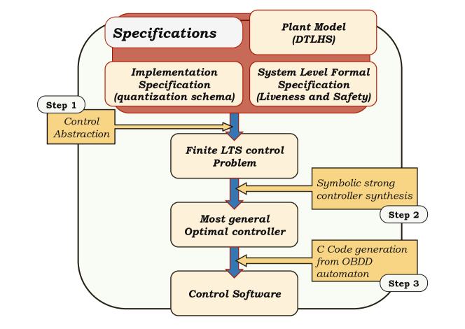
Figure 1: Control Software Synthesis Flow.

To find the quantized controller $\hat{K}$, QKS implements the symbolic synthesis algorithm in [9], based on Ordered Bynary Decision Diagrams (OBDDs) manipulation. This algorithm finds a time-optimal solution, i.e. the controller $\hat{K}$ drives the system $\hat{\cal H}$ to $\hat{G}$ always along shortest paths. The finer the control abstraction is (i.e. when the quantization schema is more precise), the better is the control strategy found. Unfortunately, such time optimal control strategies may lead to very large controllers in terms of the size of the generated C control software.

Driven by the intuition that by enabling the very same action on large regions of the state space we may decrease the control software size, we design a controller synthesis algorithm (Alg. 2 in Sect. 3.1) that gives up optimality and looks for maximal regions that can be controlled by performing the same action. We formally prove its correctness and completeness (Theor. 1 and 2 in Sect. 3.2).

Experimental results in Sect. 4 show that such a heuristic effectively mitigates the exponential growth of the controller size without having a significant impact on non-functional system level requirements such as set-up time and ripple. We accomplish this result without changing the WCET of the synthesized control software. For the inverted pendulum benchmark, by using a quantization schema with 12 bits, the size of our controller is less than $6\%$ of the size of the time optimal controller.

1.3 Related Work

Control Engineering has been studying control law design (e.g., optimal control, robust control, etc.), for more than half a century (e.g., see [8]). Also Quantized Feedback Control has been widely studied in control engineering (e.g. see [13]). However such research does not address hybrid systems and, as explained above, focuses on control law design rather than on control software synthesis. Traditionally, control engineering approaches model quantization errors as statistical noise. As a result, correctness of the control law holds in a probabilistic sense. Here instead, we model quantization errors as nondeterministic (malicious) disturbances. This guarantees system level correctness of the generated control software (not just that of the control law) with respect to any possible sequence of quantization errors.

Formal verification of Linear Hybrid Automata (LHA) [1] has been investigated in [14, 12, 29, 27]. Quantization can be seen as a sort of abstraction. In a hybrid systems formal verification context, abstractions has been widely studied (e.g., see [2, 3]), to ease the verification task. On the other hand, in control software synthesis, quantization is a design requirement since it models a hardware component (AD converter) which is part of the specification of the control software synthesis problem. As a result, clever abstractions considered in a verification setting cannot be directly used in our synthesis setting where quantization is given.

The abstraction–based approach to controller synthesis has also been broadly investigated. Based on a notion of suitable finite state abstraction (e.g. see [24]) control software synthesis for continuous time linear systems (no switching) has been implemented in the tool Pessoa [23]. On the same wavelength, [30] generates a control strategy from a finite abstraction of a Piecewise Affine Discrete Time Hybrid System (PWA-DTHS). Also the Hybrid Toolbox [6] considers PWA-DTHSs. Such tools output a feedback control law that is then passed to Matlab in order to generate control software. Finite horizon control of PWA-DTHSs has been studied using a MILP based approach (e.g. see [7]). Explicit finite horizon control synthesis algorithms for discrete time (possibly non-linear) hybrid systems have been studied in [11]. All such approaches do not account for state feedback quantization since they all assume exact (i.e. real valued) state measures. Optimal switching logic, i.e. synthesis of optimal controllers with respect to some cost function has also been widely investigated (e.g. see [17]). In this paper, we focus on non-functional sofware requirements rather than non-functional system-level requirements.

Summing up, to the best of our knowledge, no previously published result is available about model based synthesis of small footprint control software from a plant model, system level specifications and implementation specifications.

2 Control Software Synthesis

To make this paper self-contained, first we briefly summarize previous work on automatic generation of control software for Discrete Time Linear Hybrid Systems (DTLHSs) from System Level Formal Specifications. We focus on basic definitions and mathematical tools that will be useful later.

We model the controlled system (i.e. the plant) as a DTLHS (Sect. 2.3), that is a discrete time hybrid system whose dynamics is modeled as a linear predicate (Sect. 2.1) over a set of continuous as well as discrete variables. The semantics of a DTLHS is given in terms of a Labeled Transition Systems (LTSs, Sect. 2.2).

Given a plant ${\cal H}$ modeled as a DTLHS, a set of goal states $G$ (liveness specifications) and an initial region $I$, both represented as linear predicates, we are interested in finding a restriction $K$ of the behaviour of ${\cal H}$ such that in the closed loop system all paths starting in $I$ lead to $G$ after a finite number of steps. Moreover, we are interested in controllers that take their decisions by looking at quantized states, i.e. the values that the control software reads after an AD conversion. This is the quantized control problem (Sect. 2.3.1).

The quantized controller is computed by solving an LTS control problem (Sect. 2.2.1), by using a symbolic approach based on Ordered Binary Decision Diagrams (OBDDs) (Sect. 2.4.1). Finally, we briefly describe how C control software is automatically generated from the OBDD controller representation (Sect. 2.4.2).

2.1 Predicates

We denote with $[n]$ an initial segment $\{1,\ldots,n\}$ of the natural numbers. We denote with $X$ = $[x_{1},\ldots,x_{n}]$ a finite sequence of distinct variables, that we may regard, when convenient, as a set. Each variable $x$ ranges on a known (bounded or unbounded) interval ${\cal D}_{x}$ either of the reals or of the integers (discrete variables). Boolean variables are discrete variables ranging on the set $\mathbb{B}$ = {0, 1}. We denote with ${\cal D}_{X}$ the set $\prod_{x\in X}{\cal D}_{x}$. To clarify that a variable $x$ is continuous (resp. discrete, boolean) we may write $x^{r}$ (resp. $x^{d}$, $x^{b}$). Analogously $X^{r}$ ($X^{d}$, $X^{b}$) denotes the sequence of real (integer, boolean) variables in $X$. Unless otherwise stated, we suppose ${\cal D}_{X^{r}}=\mathbb{R}^{|X^{r}|}$ and ${\cal D}_{X^{d}}=\mathbb{Z}^{|X^{d}|}$. Finally, if $x$ is a boolean variable we write $\bar{x}$ for $(1-x)$.

A linear expression $L(X)$ over a list of variables $X$ is a linear combination of variables in $X$ with rational coefficients. A linear constraint over $X$ (or simply a constraint) is an expression of the form $L(X)\leq b$, where $b$ is a rational constant. In the following, we also write $L(X)\geq b$ for $-L(X)\leq-b$, $L(X)=b$ for ($L(X)\leq b$) $\wedge$ ($L(X)\geq b$), and $a\leq x\leq b$ for $x\geq a\;\land\;x\leq b$.

Predicates are inductively defined as follows. A constraint $C(X)$ over a list of variables $X$ is a predicate over $X$. If $A(X)$ and $B(X)$ are predicates over $X$, then $(A(X)\land B(X))$ and $(A(X)\lor B(X))$ are predicates over X. Parentheses may be omitted, assuming usual associativity and precedence rules of logical operators. A conjunctive predicate is a conjunction of constraints.

A valuation over a list of variables $X$ is a function $v$ that maps each variable $x\in X$ to a value $v(x)\in{\cal D}_{x}$. Given a valuation $v$, we denote with $X^{\ast}\in{\cal D}_{X}$ the sequence of values $[v(x_{1}),\ldots,v(x_{n})]$. We also call valuation the sequence of values $X^{\ast}$. A satisfying assignment to a predicate $P(X)$ is a valuation $X^{*}$ such that $P(X^{*})$ holds. If a satisfying assignment to a predicate $P$ over $X$ exists, we say that $P$ is feasible. Abusing notation, we may denote with $P$ the set of satisfying assignments to the predicate $P(X)$.

Two predicates $P$ and $Q$ over $X$ are equivalent, denoted by $P\equiv Q$, if they have the same set of satisfying assignments. Two predicates $P(X)$ and $Q(Z)$ are equisatisfiable, notation $P\simeq Q$ if $P$ is satisfiable if and only if $Q$ is satisfiable. A variable $x\in X$ is said to be bounded in $P$ if there exist $a$, $b\in{\cal D}_{x}$ such that $P(X)$ implies $a\leq x\leq b$. A predicate is bounded if all its variables are bounded.

Given a constraint $C(X)$ and a fresh boolean variable (guard) $y\not\in X$, the guarded constraint $y\to C(X)$ (if $y$ then $C(X)$) denotes the predicate $(y=0)\lor C(X)$. Similarly, we use $\bar{y}\to C(X)$ (if not $y$ then $C(X)$) to denote the predicate $(y=1)\lor C(X)$. A guarded predicate is a conjunction of either constraints or guarded constraints. It is possible to show that, if a guarded predicate $P$ is bounded, then $P$ can be transformed into an equisatisfiable conjunctive predicate.

2.2 Labeled Transition Systems

A Labeled Transition System (LTS) is a tuple ${\cal S}=(S,A,T)$ where $S$ is a (possibly infinite) set of states, $A$ is a (possibly infinite) set of actions, and $T:S\!\times\!A\!\times\!S\!\rightarrow\!\mathbb{B}$ is the transition relation of ${\cal S}$. Let $s\in S$ and $a\in A$. We denote with $\mbox{\rm Adm}({\cal S},s)$ the set of actions admissible in $s$, that is $\mbox{\rm Adm}({\cal S},s)$ = $\{a\in A\;|\;\exists s^{\prime}:T(s,a,s^{\prime})\}$ and with $\mbox{\rm Img}({\cal S},s,a)$ the set of next states from $s$ via $a$, that is $\mbox{\rm Img}({\cal S},s,a)$ = $\{s^{\prime}\in S\;|\;T(s,a,s^{\prime})\}$. A run or path for an LTS ${\cal S}$ is a sequence $\pi$ = $s_{0},a_{0},s_{1},a_{1},s_{2},a_{2},\ldots$ of states $s_{t}$ and actions $a_{t}$ such that $\forall t\geq 0$ $T(s_{t},a_{t},s_{t+1})$. The length $|\pi|$ of a finite run $\pi$ is the number of actions in $\pi$. We denote with $\pi^{(S)}(t)$ the $(t+1)$-th state element of $\pi$, and with $\pi^{(A)}(t)$ the $(t+1)$-th action element of $\pi$. That is $\pi^{(S)}(t)$ = $s_{t}$, and $\pi^{(A)}(t)$ = $a_{t}$.

2.2.1 LTS Control Problem

A controller for an LTS ${\cal S}$ is used to restrict the dynamics of ${\cal S}$ so that all states in the initial region will eventually reach the goal region. We formalize such a concept by defining the LTS control problem and its solutions. In what follows, let ${\cal S}=(S,A,T)$ be an LTS, $I$, $G$ $\subseteq$ $S$ be, respectively, the initial and goal regions.

Definition 1.

A controller for ${\cal S}$ is a function $K:S\times A\rightarrow\mathbb{B}$ such that $\forall s\in S$, $\forall a\in A$, if $K(s,a)$ then $\exists s^{\prime}\;T(s,a,s^{\prime})$. If $K(s,a)$ holds, we say that the action $a$ is enabled by $K$ in $s$.

The set of states for which at least one action is enabled is denoted by ${\rm dom}(K)$. Formally, ${\rm dom}(K)$ $=$ $\{s\in S\;|\;$$\exists a\;K(s,a)\}.$

We call a controller $K$ a control law if $K$ enables at most one action in each state. Formally, $K$ is a control law if, for all $s\in{\rm dom}(K)$, $K(s,a)$ and $K(s,b)$ implies $a=b$.

The closed loop system is the LTS ${\cal S}^{(K)}=(S,A,T^{(K)})$, where $T^{(K)}(s,a,s^{\prime})$ $=$ $T(s,a,s^{\prime})\wedge K(s,a)$.

We call a path $\pi$ fullpath [5] if either it is infinite or its last state $\pi^{(S)}(|\pi|)$ has no successors (i.e. $\mbox{\rm Adm}({\cal S},\pi^{(S)}(|\pi|))=\varnothing$). We denote with ${\rm Path}(s,a)$ the set of fullpaths starting in state $s$ with action $a$, i.e. the set of fullpaths $\pi$ such that $\pi^{(S)}(0)=s$ and $\pi^{(A)}(0)=a$. Given a path $\pi$ in ${\cal S}$, we define $j({\cal S},\pi,G)$ as follows. If there exists $n>0$ s.t. $\pi^{(S)}(n)\in G$, then $j({\cal S},\pi,G)=\min\{n\;|\;n>0\land\pi^{(S)}(n)\in G\}$. Otherwise, $j({\cal S},\pi,G)=+\infty$. We require $n>0$ since our systems are nonterminating and each controllable state (including a goal state) must have a path of positive length to a goal state. Taking ${\rm sup}\,\varnothing=+\infty$, the worst case distance of a state $s$ from the goal region $G$ is $J({\cal S},G,s)={\rm sup}\{j({\cal S},\pi,G)~{}|~{}\pi\in{\rm Path}(s,a),a\in{\rm Adm}({\cal S},s)\}$.

Figure 2: The LTS ${\cal S}$ in Example 1.

Definition 2.

An LTS control problem is a triple $\cal P$ = $({\cal S},$ $I,$ $G)$. A strong solution (or simply a solution) to ${\cal P}$ is a controller $K$ for ${\cal S}$, such that $I$ $\subseteq$ ${\rm dom}(K)$ and for all $s\in{\rm dom}(K)$, $J({\cal S}^{(K)},G,s)$ is finite.

An optimal solution to ${\cal P}$ is a solution $K^{*}$ to ${\cal P}$ such that for all solutions $K$ to ${\cal P}$, for all $s\in S$, we have $J({\cal S}^{(K^{*})},G,s)\leq J({\cal S}^{(K)},G,s)$.

The most general optimal (mgo) solution to ${\cal P}$ is an optimal solution $\bar{K}$ to ${\cal P}$ such that for all optimal solutions $K$ to ${\cal P}$, for all $s\in S$, for all $a\in A$ we have $K(s,a)$ $\rightarrow$ $\bar{K}(s,a)$. This definition is well posed (i.e., the mgo solution is unique) and $\bar{K}$ does not depend on $I$.

Example 1.

Let ${\cal S}=(S,A,T)$ be the LTS in Fig. 2, where $S=\{0,1,2,3,4\}$, $A=\{0,1\}$ and the transition relation $T$ is defined by all arrows in the picture. Let $I=S$ and let $G=\{0\}$. The controller $K$ that enables all dotted arrows in the picture, is an mgo for the control problem $({\cal S},I,G)$. The controller $K^{\prime}=K\setminus\{(0,1)\}$ that enables only the action $0$ in the state $0$, would be still an optimal solution, but not the most general. The controller $K^{\prime\prime}=K\cup\{(3,0)\}$ that enables also the action $0$ in state $3$ would be still a solution (more general than $K$), but no more optimal. As a matter of fact, in this case $J({\cal S}^{(K^{\prime\prime})},G,3)=3$, whereas $J({\cal S}^{(K)},G,3)=2$.

2.3 Discrete Time Linear Hybrid Systems

Many embedded control systems can be modeled as Discrete Time Linear Hybrid Sytems (DTLHSs) since they provide an uniform model both for the plant and for the control software.

Definition 3.

A Discrete Time Linear Hybrid System is a tuple ${\cal H}=(X,$ $U,$ $Y,$ $N)$ where:

$X$ = $X^{r}\cup X^{d}$ is a finite sequence of real ($X^{r}$) and discrete ($X^{d}$) present state variables. The sequence $X^{\prime}$ of next state variables is obtained by decorating with ^′ all variables in $X$.

$U$ = $U^{r}\cup U^{d}$ is a finite sequence of input variables.

$Y$ = $Y^{r}\cup Y^{d}$ is a finite sequence of auxiliary variables, that are typically used to model modes or “local” variables.

$N(X,U,Y,X^{\prime})$ is a conjunctive predicate over $X\cup U\cup Y\cup X^{\prime}$ defining the transition relation (next state) of the system.

A DTLHS is bounded if the predicate $N$ is bounded.

Since any bounded guarded predicate is equisatisfiable to a conjunctive predicate (see Sect. 2.1), for the sake of readability we use bounded guarded predicates to describe the transition relation of bounded DTLHSs. To this aim, we also clarify which variables are boolean, and thus may be used as guards in guarded constraints.

The semantics of DTLHSs is given in terms of LTSs as follows.

Definition 4.

Let ${\cal H}$ = ($X$, $U$, $Y$, $N$) be a DTLHS. The dynamics of ${\cal H}$ is defined by the Labeled Transition System $\mbox{\rm LTS}({\cal H})$ = (${\cal D}_{X}$, ${\cal D}_{U}$, $\tilde{N}$) where: $\tilde{N}:{\cal D}_{X}\;\times\;{\cal D}_{U}\;\times\;{\cal D}_{X}\rightarrow\mathbb{B}$ is a function s.t. $\tilde{N}(x,u,x^{\prime})\equiv\exists\;y\in{\cal D}_{Y}\;N(x,u,y,x^{\prime})$. A state $x$ for ${\cal H}$ is a state $x$ for $\mbox{\rm LTS}({\cal H})$ and a run (or path) for ${\cal H}$ is a run for $\mbox{\rm LTS}({\cal H})$.

Example 2.

Let T be a positive constant (sampling time). We define the DTLHS ${\cal H}$ $=$ $(\{x\},\{u\},$ $\varnothing$, $N)$ where $x$ is a continuous variable, $u$ is a boolean variable, and $N(x,u,x^{\prime})$ $\equiv$ $[\overline{u}\rightarrow x^{\prime}=x+(\frac{5}{4}-x)T]\land[u\rightarrow x^{\prime}=x+(x-\frac{3}{2})T]$. Since $N(\frac{5}{4},0,\frac{5}{4})$ holds, the infinite path $\pi_{0}=\frac{5}{4},0,\frac{5}{4},0\ldots$ is a run in $LTS({\cal H})=(\mathbb{R},\{0,1\},N)$.

2.3.1 DTLHS Control Problem

A DTLHS control problem $({\cal H},I,G)$ is defined as the LTS control problem ($\mbox{\rm LTS}(\cal H)$, $I$, $G$). To manage real valued variables, in classical control theory the concept of quantization is introduced (e.g., see [13]). Quantization is the process of approximating a continuous interval by a set of integer values. In the following we formally define a quantized feedback control problem for DTLHSs.

A quantization function $\gamma$ for a real interval $I=[a,b]$ is a non-decreasing function $\gamma:I\mapsto\mathbb{Z}$ such that $\gamma(I)$ is a bounded integer interval. We extend quantizations to integer intervals, by stipulating that in such a case the quantization function is the identity function.

Definition 5.

Let ${\cal H}=(X,U,Y,N)$ be a DTLHS, and let $W=X\cup U\cup Y$. A quantization ${\cal Q}$ for $\cal H$ is a pair $(A,\Gamma)$, where:

$A$ is a predicate over $W$ that explicitely bounds each variable in $W$. For each $w\in W$, we denote with $A_{w}$ its admissible region and with $A_{W}$ $=$ $\prod_{w\in W}A_{w}$.

$\Gamma$ is a set of maps $\Gamma=\{\gamma_{w}$ $|$ $w\in W$ and $\gamma_{w}$ is a quantization function for $A_{w}\}$.

Let $W=[w_{1},\ldots w_{k}]$ and $v=[v_{1},\ldots v_{k}]\in A_{W}$. We write $\Gamma(v)$ for the tuple $[\gamma_{w_{1}}(v_{1}),\ldots\gamma_{w_{k}}(v_{k})]$.

A control problem admits a quantized solution if control decisions can be made by just looking at quantized values. This enables a software implementation for a controller.

Definition 6.

Let ${\cal H}=(X,U,Y,N)$ be a DTLHS, ${\cal Q}=(A,\Gamma)$ be a quantization for ${\cal H}$ and ${\cal P}=({\cal H},I,G)$ be a DTLHS control problem. A ${\cal Q}$ Quantized Feedback Control (QFC) solution to ${\cal P}$ is a solution $K(x,u)$ to ${\cal P}$ such that $K(x,u)=\hat{K}(\Gamma(x),\Gamma(u))$ where $\hat{K}:\Gamma(A_{X})\times\Gamma(A_{U})$ $\rightarrow$ $\mathbb{B}$.

Example 3.

Let ${\cal H}$ be the DTLHS in Ex. 2. Let ${\cal P}$ = (${\cal H}$, $I$, $G$) be a control problem, where $I\equiv-2\leq x\leq 2.5$, and $G\equiv\varepsilon\leq x\leq\varepsilon$, for some $\varepsilon\in\mathbb{R}$. If the sampling time $T$ is small enough with respect to $\varepsilon$ (for example $T<\frac{\varepsilon}{10})$, the controller: $K(x,u)=(-2\leq x\leq 0\;\land\;\overline{u})\;\lor\;(0\leq x\leq\frac{11}{8}\;\land\;u)\;\lor\;(\frac{11}{8}\leq x\leq 2.5\;\land\;\overline{u})$ is a solution to $({\cal H},I,G)$. Observe that any controller $K^{\prime}$ such that $K^{\prime}(\frac{5}{4},0)$ holds is not a solution, because in such a case ${\cal H}^{(K)}$ may loop forever along the path $\pi_{0}$ of Ex. 2.

Let us consider the quantization $(A,\Gamma)$ where $A=I$ and $\Gamma$ = $\{\gamma_{x}\}$ and $\gamma_{x}(x)=\lfloor x\rfloor$. The set $\Gamma(A_{x})$ of quantized states is the integer interval $[-2,2]$. No solution can exist, because in state $1$ either enabling action $1$ or $0$ allows infinite loops to be potentially executed in the closed loop system. The controller $K$ above can be obtained as a quantized controller decreasing the quantization step, for example by taking $\tilde{\Gamma}$ = $\{\tilde{\gamma}_{x}\}$ where $\tilde{\gamma}_{x}(x)=\lfloor 8x\rfloor$.

2.4 Control Software Generation

Quantized controllers can be computed by solving LTS control problems: the QKS control software synthesis procedure consists of building a suitable finite state abstraction (control abstraction) $\hat{\cal H}$ induced by the quantization of a plant modeled as a DTLHS ${\cal H}$, computing an abstraction $\hat{I}$ (resp. $\hat{G}$) of the initial (resp. goal) region $I$ (resp. $G$) so that any solution to the LTS control problem $(\hat{\cal H},\hat{I},\hat{G})$ is a finite representation of a solution to $({\cal H},I,G)$. In [20], we give a constructive sufficient condition ensuring that the controller computed for $\hat{\cal H}$ is indeed a quantized controller for ${\cal H}$.

2.4.1 Symbolic Controller Synthesis

Control abstractions for bounded DTLHSs are finite LTSs. For example, a typical quantization is the uniform quantization which consists in dividing the domain of each state variable $x$ into $2^{b_{x}}$ equal intervals, where $b_{x}$ is the number of bits used by AD conversion. Therefore, the abstraction of a DTLHS induced by a uniform quantization has $2^{B}$ states, where $B=\sum_{x\in X}b_{x}$. By coding states and actions as sequences of bits, a finite LTS can be represented as an OBDD representing set of states and the transition relation by using their characteristic functions.

The QKS control synthesis procedure implements the function mgoCtr in Alg. 1, which adapts the algorithm presented in [9]. Starting from goal states, the most general optimal controller is found incrementally adding at each step to the set of states $D(s)$ controlled so far, the strong preimage of $D(s)$, i.e. the set of states for which there exists at least an action $a$ that drives the system to $D(s)$, regardless of possible nondeterminism.

Algorithm 1 Symbolic Most General Optimal Controller Synthesis

0.  An LTS control problem $({\cal S},I,G)$, ${\cal S}=(S,A,T)$.

0.  mgoCtr(${\cal S},I,G$)

1.  $K(s,a)\leftarrow 0$, $D(s)\leftarrow G(s)$, $\tilde{D}(s)\leftarrow 0$

2.  while $D(s)\neq\tilde{D}(s)$ do

3.     $F(s,a)\leftarrow\exists s^{\prime}\;T(s,a,s^{\prime})\land\forall s^{\prime}\;[T(s,a,s^{\prime})\Rightarrow D(s^{\prime})]$

4.     $K(s,a)\leftarrow K(s,a)\lor(F(s,a)\land\not\exists a\;K(s,a))$

5.     $\tilde{D}(s)\leftarrow D(s)$, $D(s)\leftarrow D(s)\lor\exists a\;K(s,a)$

6.  return $\langle\forall s\;[I(s)\Rightarrow\exists a\;K(s,a)],\exists a\;K(s,a),K(s,a)\rangle$

Figure 3: OBDD for $F$.

int ctrlLaw(unsigned char *x){ int act=0; L_v1: if (x[2]==1) goto L_v3; else { act = !act; goto L_v2;} L_v2: if (x[1]==1) goto L_v4; else { act = !act; goto L_v4;} L_v3: if (x[1]==1) return act; else goto L_v4; L_v4: if (x[0]==1) return act; else { act = !act; return act;} } Figure 4: C control software.

2.4.2 C Code Generation

The output of the function mgoCtr is an OBDD $K$ representing an mgo as a relation $K(x,u)$. Let $k$ be the number of bits used to represent the set of actions. We are interested in a control law $F=[f_{1},\ldots,f_{k}]$ such that $K(x,F(x))$ holds for all $x$ [28]. We first compute $k$ OBDDs $f_{1},\ldots f_{k}$ representing $F$. For any $f_{i}$, by replacing each OBDD node with an if- then-else block and each OBDD edge with a goto statement, we obtain a C function f_i that implements the boolean function represented by $f_{i}$. Therefore, the size of f_i is proportional to the number of nodes in $f_{i}$. Its WCET is proportional to the height of $f_{i}$, since any computation of f_i corresponds to going through a path of $f_{i}$. As a consequence, the WCET of the control software turns out to be linear in the number of bits of the quantization schema. The C function ctrLaw is obtained by translating the $k$ OBDDs representing $F$, whereas ctrReg is obtained by translating the OBDD representing the characteristic function of ${\rm dom}(K)$. The actual code implementing control software is slightly more complicated to account for node sharing among OBDDs $f_{1},\ldots,f_{k}$. Full details about the control software generation can be found in [21].

Example 4.

Let ${\cal P}=({\cal S},I,G)$ be the control problem in Ex. 1. The five states of ${\cal S}$ can be represented by three boolean variables ($x_{0},x_{1},x_{2}$). Taking as input ${\cal P}$, mgoCtr computes the mgo $K$ given in Ex. 1. The control law $F$ is the OBDD depicted in Fig. 4. In Fig. 4, it is shown a snapshot of the control software generated for $F$.

3 Small Controllers Synthesis

Within the framework defined in the previous section, when finer (i.e. with more bits) quantization schemas are considered, better controllers are found, in terms of set-up time and ripple (see Sect. 4). On the other hand, the exponential growth of control software size is one of the main obstacles to overcome in order to make model based control software synthesis viable on large problems. As explained in Sect. 2.4.2, the size of the control software is proportional to the size of the OBDD computed by the function mgoCtr in Sect. 2.4.1. To reduce the number of nodes of such an OBDD, we devise a heuristic aimed at increasing OBDD node sharing by looking for control laws that are constant on large regions of the state space.

While optimal controllers implement smart control strategies that in each state try to find the best action to drive the system to the goal region, the function smallCtr in Sect. 3.1 looks for more “regular” controllers that enable the same action in as large as possible regions of the state space.

Finally, note that changing the control synthesis algorithm does not change the WCET of the generated control software since it only depends on the number of quantization bits (Sect. 2.4.2).

3.1 Control Synthesis Algorithm

Our controller synthesis algorithm is shown in Alg. 2. To obtain a succinct controller, the function smallCtr modifies the mgoCtr preimage computation of set of states $D$ by finding maximal regions of states from which the system reaches $D$ in one or more steps by repeatedly performing the same action. This involves finding at each step a family of fixpoints: for each action $a$, $E(s,a)$ is the maximal set of states from which $D$ is reachable by repeatedly performing the action $a$ only.

The function smallCtr(${\cal S},I,G$) computes a solution $K$ to the control problem (${\cal S},I,G$) (Theor. 1), such that ${\rm dom}(K)$ is maximal with respect to any other solution (Theor. 2).

In Alg. 2 $K(s,a)$ denotes the OBDD that represents the controller computed so far, $D(s)$ the OBDD that represents its domain, and $\tilde{D}(s)$ the domain of the controller computed at the previous iteration. The computation starts by initializing $K(s,a)$ and its domain $D(s)$ to the empty OBDD, that corresponds to the always undefined function and the empty set (line 1).

At each iteration of the outer loop (lines 2–11), a target set of states $O(s)$ is considered (line 3): $O(s)$ consists of goal states $G(s)$ and the set $D(s)$ of already controlled states. The inner loop (lines 4–7) computes, for each action $a$, the maximal set of states $E(s,a)$ that can reach the target set $O(s)$ by repeatedly performing the action $a$ only. For any action $a_{0}$, $E(s,a_{0})$ is the mgo of the control problem $({\cal S}^{\prime},I,O)$, where the LTS ${\cal S}^{\prime}=(S,\{a_{0}\},T^{\prime})$ is obtained by restricting the dynamics of ${\cal S}$ to the action $a_{0}$.

After that, $K$ is updated by adding to it state-action pairs in $E(s,a)$. Instead of simply computing $K(s,a)\!\leftarrow\!K(s,a)\lor E(s,a)$, to keep the controller smaller, function smallCtr avoids to add to $K$ possible intersections between any pair of sets $E(s,a)$ and $E(s,b)$ for $a\neq b$ (line 9). As a consequence, the resulting controller $K$ is a control law, i.e. it enables just one action in a given state $s$.

The order in which the loop in lines 8–9 enumerates the set of actions gives priority to actions that are considered before. Let $a_{0},a_{1},\ldots,a_{n}$ be the sequence of actions as enumerated by the for loop. If there exists at least one action $a$ such that $E(s,a)$ holds, then we will have that $K(s,a_{k})$ holds only for a certain $a_{k}$ such that $k=\min\{i~{}|~{}E(s,a_{i})\}$. In many control problems, this is useful as it allow one to give priority to some actions, e.g. in order to prefer “low power” actions.

The computation ends when no new state is added to the controllable region, i.e. when $D(s)$, is the same as $\tilde{D}(s)$.

Algorithm 2 Symbolic Small Controller Synthesis

0.  LTS control problem $({\cal S},I,G)$, with LTS ${\cal S}=(S,A,T)$

0.  smallCtr(${\cal S},I,G$)

1.  $K(s,a)\leftarrow 0$, $D(s)\leftarrow 0$

2.  repeat

3.     $O(s)\leftarrow D(s)\;\lor\;G(s)$, $E(s,a)\leftarrow 0$

4.     repeat

5.        $F(s,a)\!\leftarrow\!\exists s^{\prime}T(s,a,s^{\prime})\!\land\!\forall s^{\prime}[T(s,a,s^{\prime})\!\Rightarrow\!E(s^{\prime},a)\!\lor\!O(s^{\prime})]$

6.        $\tilde{E}(s,a)\leftarrow E(s,a)$, $E(s,a)\leftarrow E(s,a)\,\lor\,F(s,a)$

7.     until $E(s,a)=\tilde{E}(s,a)$

8.     for all $\tilde{a}\in A$ do

9.        $K(s,a)\leftarrow K(s,a)\lor(E(s,a)\land a=\tilde{a}\,\land\not\exists b\;K(s,b))$

10.     $\tilde{D}(s)\leftarrow D(s)$, $D(s)\leftarrow D(s)\lor\exists aK(s,a)$

11.  until $D(s)=\tilde{D}(s)$

12.  return $\langle\forall s\;[I(s)\Rightarrow\exists aK(s,a)],\exists aK(s,a),K(s,a)\rangle$

Example 5.

Let ${\cal P}$ be the control problem described in Ex. 1. The first iteration of Alg. 2 computes the predicate $E(s,a)$ that holds on the set $\{(0,0),(0,1),(1,0),(2,0),(3,0),(4,1)\}$, that is $E(s,a)=E(s,0)\,\lor\,E(s,1)$, where the set of pairs that satisfies $E(s,0)$ is $\{(0,0),(1,0),(2,0),(3,0)\}$ and the set of pairs that satisfies $E(s,1)$ is $\{(0,1),(4,1)\}$. Depending on the order in which the for loop in lines 8–9 enumerates the set of actions, in the state 0 the resulting controller $K^{*}$ enables the action 0 ($K^{*}(s,a)=E(s,0)\cup(E(s,1)\setminus\{(0,1)\})$) or the action 1 ($K^{*}(s,a)=E(s,1)\cup(E(s,0)\setminus\{(0,0)\})$). Observe that, in any case, $K^{*}$ is not optimal. An optimal controller would enable the transition $T(3,1,1)$ rather than $T(3,0,2)$ (see Ex. 1).

The OBDD representing the control law $F$ such that $K^{*}(x,F(x))$ holds, is depicted in Fig. 6. It has 3 nodes, instead of the 4 nodes required for the OBDD representation of the control law (Fig. 4) obtained from the controller $K$ given in Ex. 1. Accordingly, the corresponding C code in Fig. 6 has 3 if-then-else blocks, instead of the 4 in the C code of Fig. 4.

Remark 1.

Let $\pi$ $=$ $s_{0},a_{0},$ $s_{1},a_{1},$ $\ldots,$ $a_{n-1},s_{n}$ be a path. An action switch in $\pi$ occurs whenever $a_{i}\not=a_{i+1}$. Controllers generated by Alg. 2 implement control strategies with a very low number of switches. In many systems this is a desirable property. A “switching optimal” control strategy cannot be, however, implemented by a memoryless state-feedback control law. As an example, take again the control problem ${\cal P}$ described in Ex. 1. The controller defined by $E(s,a)$ in Ex. 5 contains all switch optimal paths. However, to minimize the number of switches along the paths going through state $0$, a controller should enable action $0$ when coming from state 1, action $1$ when coming from $4$, and repeat the last action ($0$ or $1$) when the system is executing the self-loops in state $0$. In other words, only a feedback controller with memory can implement this control strategy.

Figure 5: OBDD for $F^{*}$.

int ctrlLaw(unsigned char *x){ int act=0; L_v1: if (x[2]==1) goto L_v2; else return act; L_v2: if (x[1]==1) return act; else goto L_v3; L_v3: if (x[0]==1) return act; else { act = !act; return act;} } Figure 6: C code for $F^{*}$.

3.2 Synthesis Algorithm Correctness
and Completeness

In the following, we establish the correctness of Alg. 2, by showing that the controller computed by smallCtr is indeed a solution to the control problem given as input (Theor. 1), and its completeness, in the sense that the domain of the computed controller is maximal with respect to the domain of any other solution (Theor. 2).

Theorem 1.

Let ${\cal S}=(S,A,T)$ be an LTS, and $I,G\subseteq S$ be two sets of states. If ${\textsl{smallCtr}}($S, I, G$)$ returns the tuple $\langle\mbox{\sc True},$ $D,$ $K\rangle$, then $K$ is a solution to the control problem $({\cal S},I,G)$.

Proof.

If ${\textsl{smallCtr}}($S, I, G$)$ returns the tuple $\langle\mbox{\sc True},$ $D,$ $K\rangle$, clearly $I\subseteq{\rm dom}(K)$ (see Alg. 2, line12). We have to show that, for all $s\in{\rm dom}(K)$, $J({\cal S}^{(K)},G,s)$ is finite.

First of all, we show that at the end of the inner repeat loop of smallCtr (lines 4–7), if $E(s,a)$ holds, then we have that $J({\cal S}^{(E)},$ $O,$ $s)$ is finite. We proceed by induction on the number of iteration of the inner repeat loop. Denoting with $F_{i}(s,a)$ the predicate $F(s,a)$ computed in line 5 during the $i$-th iteration, we will show that if $F_{n}(s,a)$ holds, then $J({\cal S}^{(E)},$ $O,$ $s)=n$. If $F_{1}(s,a)$ holds, then for all $s^{\prime}$ such that $T(s,a,s^{\prime})$, $s^{\prime}$ belongs to $O$, and hence $J({\cal S}^{(E)},$ $O,$ $s)=1$. Along the same lines, if $F_{n+1}(s,a)$ holds, then $J({\cal S}^{(E)},$ $F_{n},$ $s)=1$, and by applying induction hypothesis, $J({\cal S}^{(E)},$ $O,$ $s)=n+1$. As for termination, we have that if $\tilde{E}(s,a)\neq E(s,a)$ then at least one new state has been included in $E(s,a)$. Thus the function $|S|-|{\rm dom}(E)|$ is strictly positive and strictly decreasing at each iteration.

The outer repeat loop behaves in a similar way. Denoting with $E_{i}(s,a)$ the predicate $E(s,a)$ computed in line 3 during the $i$-th iteration, if $s\in{\rm dom}(K)$, then $E_{i}(s,a)$ holds for some $i$ and some $a$. We prove the statement of the theorem by induction on $i$. If $i\!=\!1$, we have that $O(s)\!=\!G(s)$ and that $J({\cal S}^{(E_{1})},$ $O,$ $s)$ is finite, and hence trivially $J({\cal S}^{(K)},$ $G,$ $s)$ is finite. If $i>1$, then we have that $J({\cal S}^{(E_{i})},$ ${\rm dom}(E_{i-1}),$ $s)$ is finite. Since, by inductive hypothesis, also $J({\cal S}^{(E_{i-1})},$ $O,$ $s)$ is finite, we have that $J({\cal S}^{(K)},$ $G,$ $s)$ $\leq$ $J({\cal S}^{(E_{i})},$ ${\rm dom}(E_{i-1}),$ $s)$ + $J({\cal S}^{(E_{i-1})},$ $O,$ $s)$ is finite. ∎

Theorem 2.

Let ${\cal S}=(S,A,T)$ be an LTS, and $I,G\subseteq S$ be two sets of states. If ${\textsl{smallCtr}}($S, I, G$)$ returns the tuple $\langle\mbox{\sc True},$ $D,$ $K\rangle$, then $D={\rm dom}(K)$ is the maximal controllable region, i.e. for any other solution $K^{*}$ to the control problem (${\cal S},I,G$) we have ${\rm dom}(K^{*})\subseteq{\rm dom}(K)$.

Proof.

Let ${\rm dom}_{n}(K)=\{s~{}|~{}J({\cal S}^{(K)},s,G)=n\}$. We will show by induction that, for all $n$, ${\rm dom}_{n}(K^{*})\subseteq{\rm dom}(K)$.

$(n=1)$ Let $s\in{\rm dom}_{1}(K^{*})$. Then $\mbox{\rm Adm}({\cal S},s)\not=\varnothing$ and there exists at least one action $a\in{\rm Adm}({\cal S},s)$ such that $K^{*}(s,a)$ holds. Thus, for all $s^{\prime}$ such that $T(s,a,s^{\prime})$ we have that $s^{\prime}\in G$. But this means that $F(s,a)$ holds (Alg. 2, line 5) and therefore $K(s,a)$ holds. Hence $s\in{\rm dom}(K)$.

$(n>1)$ Let $s\in{\rm dom}_{n}(K^{*})$. Then $\mbox{\rm Adm}({\cal S},s)\not=\varnothing$ and there exists at least an action $a\in{\rm Adm}({\cal S},s)$ such that $K^{*}(s,a)$ holds. Thus, for all $s^{\prime}$ such that $T(s,a,s^{\prime})$ we have that $s^{\prime}\in{\rm dom}_{n-1}(K^{*})$. By inductive hypothesis, ${\rm dom}_{n\!-\!1}(K^{*})\!\subseteq\!{\rm dom}(K)$. Therefore, for all $s^{\prime}$ such that $T(s,a,s^{\prime})$ we have that $s^{\prime}\!\in\!{\rm dom}(K)$. Let us suppose that $s\not\in{\rm dom}(K)$. But this implies that $\mbox{\rm Img}({\cal S},s,a)$ $\not\subseteq{\rm dom}(K)$, otherwise Alg. 2 would not terminated before adding $s$ to $E(s,a)$ at some iteration. This leads to a contradiction, because $\mbox{\rm Img}({\cal S},s,a)$ $\subseteq$ ${\rm dom}_{n-1}(K^{*})\subseteq{\rm dom}(K)$. ∎

4 Experimental Results

In this section we present our experiments that aim at evaluating the effectiveness of our control software synthesis technique. We mainly evaluate the control software size reduction and the impact on other non-functional control software requirements such as set-up time (optimality) and ripple.

We implemented smallCtr in the C programming language using the CUDD [10] package for OBDD based computations. The resulting tool, QKS${}^{\,\sf sc}$, extends the tool QKS by adding the possibility of synthesising control software (step 2 in Fig. 1) by using smallCtr instead of the mgo controller synthesis mgoCtr.

In Sect. 4.1 and  4.2 we will present the DTLHS models of the inverted pendulum and the multi-input buck DC-DC converter, on which our experiments focus. In Sect. 4.3 we give the details of the experimental setting, and finally, in Sect. 4.4, we discuss experimental results.

4.1 The Inverted Pendulum as a DTLHS

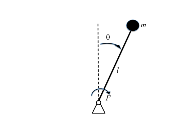
Figure 7: Inverted Pendulum with Stationary Pivot Point.

The inverted pendulum [19] (see Fig. 7) is modeled by taking the angle $\theta$ and the angular velocity $\dot{\theta}$ as state variables. The input of the system is the torquing force $u\cdot F$, that can influence the velocity in both directions. Here, the variable $u$ models the direction and the constant $F$ models the intensity of the force. Differently from [19], we consider the problem of finding a discrete controller, whose decisions may be only “apply the force clockwise” ($u=1$), “apply the force counterclockwise” ($u=-1$)”, or “do nothing” ($u=0$). The behaviour of the system depends on the pendulum mass $m$, the length of the pendulum $l$, and the gravitational acceleration $g$. Given such parameters, the motion of the system is described by the differential equation $\ddot{\theta}=\dfrac{g}{l}\sin\theta+\dfrac{1}{ml^{2}}uF$. In order to obtain a state space representation, we consider the following normalized system, where $x_{1}$ is the angle $\theta$ and $x_{2}$ is the angular speed $\dot{\theta}$:

$$\left\{\begin{array}[]{l}\dot{x}_{1}=x_{2}\\ \dot{x}_{2}=\dfrac{g}{l}\sin x_{1}+\dfrac{1}{ml^{2}}uF\end{array}\right.$$ (1)

The discrete time model obtained from the equations in (1) by introducing a constant $T$ that models the sampling time is:

$$(x^{\prime}_{1}=x_{1}+Tx_{2})\,\land\,(x^{\prime}_{2}=x_{2}+T{g\over l}\sin x_{1}+T{1\over ml^{2}}uF)$$

that is not linear, as it contains the function $\sin x_{1}$. A linear model can be found by under- and over-approximating the non linear function $\sin x$. In our experiments (Sect. 4), we will consider the linear model obtained as follows.

First of all, in order to exploit sinus periodicity, we consider the equation $x_{1}=2\pi y_{k}+y_{\alpha}$, where $y_{k}$ represents the period in which $x_{1}$ lies and $y_{\alpha}\in[-\pi,\pi]$ represents the actual $x_{1}$ inside a given period. Then, we partition the interval $[-\pi,\pi]$ in four intervals: $I_{1}$ $=$ $\left[-\pi,-\dfrac{\pi}{2}\right]$, $I_{2}$ $=$ $\left[-\dfrac{\pi}{2},0\right]$, $I_{3}$ $=$ $\left[0,\dfrac{\pi}{2}\right]$, $I_{4}$ $=$ $\left[\dfrac{\pi}{2},\pi\right]$. In each interval $I_{i}$ ($i\in[4]$), we consider two linear functions $f_{i}^{+}(x)$ and and $f_{i}^{-}(x)$, such that for all $x\in I_{i}$, we have that $f_{i}^{-}(x)\leq\sin x\leq f_{i}^{+}(x)$. As an example, $f_{1}^{+}(y_{\alpha})$ $=$ $-0.637y_{\alpha}-2$ and $f_{1}^{-}(y_{\alpha})$ $=$ $-0.707y_{\alpha}-2.373$.

Let us consider the set of fresh continuous variables $Y^{r}$ $=$ $\{y_{\alpha},$ $y_{\sin}\}$ and the set of fresh discrete variables $Y^{d}=\{y_{k},y_{q},$ $y_{1},y_{2},$ $y_{3},y_{4}\}$, with $y_{1},\ldots,y_{4}$ being boolean variables. The DTLHS model ${\cal I}_{F}$ for the inverted pendulum is the tuple $(X,U,$ $Y,N)$, where $X=\{x_{1},x_{2}\}$ is the set of continuous state variables, $U=\{u\}$ is the set of input variables, $Y=Y^{r}\,\cup\,Y^{d}$ is the set of auxiliary variables, and the transition relation $N(X,U,Y,X^{\prime})$ is the following predicate:

$$\begin{array}[]{l}(x^{\prime}_{1}=x_{1}+2\pi y_{q}+Tx_{2})\,\land\,(x^{\prime}_{2}=x_{2}+T\dfrac{g}{l}y_{\sin}+T\dfrac{1}{ml^{2}}uF)\\[6.0pt] \hskip 8.5359pt\land\,\bigwedge_{i\in[4]}y_{i}\rightarrow f_{i}^{-}(y_{\alpha})\leq y_{\sin}\leq f_{i}^{+}(y_{\alpha})\\[6.0pt] \hskip 8.5359pt\land\,\bigwedge_{i\in[4]}y_{i}\rightarrow y_{\alpha}\in I_{i}\land\sum_{i\in[4]}y_{i}\geq 1\\[6.0pt] \hskip 8.5359pt\land\;x_{1}=2\pi y_{k}+y_{\alpha}\;\land\;-\pi\leq x_{1}^{\prime}\leq\pi\end{array}$$

Overapproximations of the system behaviour increase system nondeterminism. Since ${\cal I}_{F}$ dynamics overapproximates the dynamics of the non-linear model, the controllers that we synthesize are inherently robust, that is they meet the given closed loop requirements notwithstanding nondeterministic small disturbances such as variations in the plant parameters. Tighter overapproximations of non-linear functions makes finding a controller easier, whereas coarser overapproximations makes controllers more robust.

The typical goal for the inverted pendulum is to turn the pendulum steady to the upright position, starting from any possible initial position, within a given speed interval.

4.2 Multi-input Buck DC-DC Converter

Figure 8: Multi-input Buck DC-DC Converter.

The multi-input buck DC-DC converter [25] in Fig. 8 is a mixed-mode analog circuit converting the DC input voltage ($V_{i}$ in Fig.  8) to a desired DC output voltage ($v_{O}$ in Fig.  8). As an example, buck DC-DC converters are used off-chip to scale down the typical laptop battery voltage (12-24) to the just few volts needed by the laptop processor (e.g. [26]) as well as on-chip to support Dynamic Voltage and Frequency Scaling (DVFS) in multicore processors (e.g. [18]). The typical software based approach (e.g. see [26]) is to control the switches $u_{1},\ldots,u_{n}$ in Fig. 8 (typically implemented with a MOSFET) with a microcontroller.

In such a converter there are $n$ power supplies with voltage values $V_{1},\ldots,V_{n}$, $n$ switches with voltage values $v_{1}^{u},\ldots,v_{n}^{u}$ and current values $I_{1}^{u},\ldots,I_{n}^{u}$, and $n$ input diodes $D_{0},\ldots,D_{n-1}$ with voltage values $v_{0}^{D},\ldots,v_{n-1}^{D}$ and current $i_{0}^{D},\ldots,i_{n-1}^{D}$ (in the following, we will write $v_{D}$ for $v_{0}^{D}$ and $i_{D}$ for $i_{0}^{D}$).

The circuit state variables are $i_{L}$ and $v_{C}$. However we can also use the pair $i_{L}$, $v_{O}$ as state variables in the DTLHS model since there is a linear relationship between $i_{L}$, $v_{C}$ and $v_{O}$, namely: $v_{O}\;=\;\frac{r_{C}R}{r_{C}+R}i_{L}+\frac{R}{r_{C}+R}v_{C}$. We model the $n$-input buck DC-DC converter with the DTLHS ${\cal B}_{n}$ = ($X$, $U$, $Y$, $N$), with $X=[i_{L}$, $v_{O}]$, $U=[u_{1}$, $\ldots$, $u_{n}]$, $Y=[v_{D}$, $v_{1}^{D}$, $\ldots,v_{n-1}^{D}$, $i_{D}$, $q_{0}$, $\ldots$, $q_{n-1}$, $I_{1}^{u}$, $\ldots$, $I_{n}^{u}$, $v_{1}^{u}$, $\ldots$, $v_{n}^{u}]$. From a simple circuit analysis we have the following equations:

$$\begin{array}[]{rcl}\dot{i}_{L}&=&a_{1,1}i_{L}+a_{1,2}v_{O}+a_{1,3}v_{D}\\[6.0pt] \dot{v}_{O}&=&a_{2,1}i_{L}+a_{2,2}v_{O}+a_{2,3}v_{D}\\[3.0pt] \end{array}$$

where the coefficients $a_{i,j}$ depend on the circuit parameters $R$, $r_{L}$, $r_{C}$, $L$ and $C$ in the following way: $a_{1,1}=-\frac{r_{L}}{L}$, $a_{1,2}=-\frac{1}{L}$, $a_{1,3}=-\frac{1}{L}$, $a_{2,1}=\frac{R}{r_{c}+R}[-\frac{r_{c}r_{L}}{L}+\frac{1}{C}]$, $a_{2,2}=\frac{-1}{r_{c}+R}[\frac{r_{c}R}{L}+\frac{1}{C}]$, $a_{2,3}=-\frac{1}{L}\frac{r_{c}R}{r_{c}+R}$. Using a discrete time model with sampling time $T$ (writing $x^{\prime}$ for $x(t+1)$) we have:

$${i^{\prime}_{L}} = (1+Ta_{1,1})i_{L}+Ta_{1,2}v_{O}+Ta_{1,3}v_{D}$$

$${v^{\prime}_{O}} = Ta_{2,1}i_{L}+(1+Ta_{2,2})v_{O}+Ta_{2,3}v_{D}.$$

The algebraic constraints stemming from the constitutive equations of the switching elements are the following:

$$\begin{array}[]{ccc}q_{0}\rightarrow(v_{D}=R_{\rm on}i_{D})\!&\!\bar{q}_{0}\rightarrow(v_{D}=R_{\rm off}i_{D})\!&\!v_{D}=v_{n}^{u}-V_{n}\\[6.0pt] q_{0}\rightarrow(i_{D}\geq 0)\!&\!\bar{q}_{0}\rightarrow(v_{D}\leq 0)\!&\!i_{L}=i_{D}+\sum_{i=1}^{n}I_{i}^{u}\\[6.0pt] \lx@intercol\hfil\begin{array}[]{lr}\bigwedge_{i\in[n-1]}q_{i}\rightarrow(v_{i}^{D}=R_{\rm on}I_{i}^{u}){}&~{}\bigwedge_{i\in[n-1]}\bar{q}_{i}\rightarrow(v_{i}^{D}=R_{\rm off}I_{i}^{u})\end{array}\hfil\lx@intercol\\[6.0pt] \lx@intercol\hfil\begin{array}[]{lr}\bigwedge_{i\in[n-1]}q_{i}\rightarrow(I_{i}^{u}\geq 0){}&~{}\bigwedge_{i\in[n-1]}\bar{q}_{i}\rightarrow(v_{i}^{D}\leq 0)\end{array}\hfil\lx@intercol\\[6.0pt] \lx@intercol\hfil\begin{array}[]{lr}\bigwedge_{j\in[n]}u_{j}\rightarrow(v_{j}^{u}=R_{\rm on}I_{j}^{u}){}&~{}\bigwedge_{j\in[n]}\bar{u}_{j}\rightarrow(v_{j}^{u}=R_{\rm off}I_{j}^{u})\end{array}\hfil\lx@intercol\\[6.0pt] \lx@intercol\hfil\bigwedge_{i\in[n]}v_{D}=v_{i}^{u}+v_{i}^{D}-V_{i}\hfil\lx@intercol\end{array}$$

4.3 Experimental Settings

All experiments have been carried out on an Intel(R) Xeon(R) CPU @ 2.27GHz, with 23GiB of RAM, Kernel: Linux 2.6.32-5-686-bigmem, distribution Debian GNU/Linux 6.0.3 (squeeze).

As in [19], we set pendulum parameters $l$ and $m$ in such a way that $\frac{g}{l}=1$ (i.e. $l=g$) and $\frac{1}{ml^{2}}=1$ (i.e. $m=\frac{1}{l^{2}}$). As for the quantization, we set $A_{x_{1}}=[-1.1\pi,1.1\pi]$ and $A_{x_{2}}=[-4,4]$, and we define $A_{{\cal I}_{F}}=A_{x_{1}}\times A_{x_{2}}\times A_{u}$. The goal region is defined by the predicate $G_{{\cal I}_{F}}(X)\equiv(-\rho\leq x_{1}\leq\rho)\,\land\,(-\rho\leq x_{2}\leq\rho)$, where $\rho\in\{0.05,0.1\}$, and the initial region is defined by the predicate $I_{{\cal I}_{F}}(X)\equiv(-\pi\leq x_{1}\leq\pi)\,\land\,(-4\leq x_{2}\leq 4$).

In the multi-input buck DC-DC converter with $n$ inputs ${\cal B}_{n}$, we set constant parameters as follows: $L=2\cdot 10^{-4}$ H, $r_{L}=0.1$ ${\rm\Omega}$, $r_{C}=0.1$ ${\rm\Omega}$, $R=5$ ${\rm\Omega}$, $C=5\cdot 10^{-5}$ F, $R_{\rm on}=0$ ${\rm\Omega}$, $R_{\rm off}=10^{4}$ ${\rm\Omega}$, and $V_{i}=10i$ V for $i\in[n]$. As for the quantization, we set $A_{i_{L}}=[-4,4]$ and $A_{v_{O}}=[-1,7]$, and we define $A_{{\cal B}_{n}}=A_{i_{L}}\times A_{v_{O}}\times A_{u_{1}}\times\ldots\times A_{u_{n}}$. The goal region is defined by the predicate $G_{{\cal B}_{n}}(X)\equiv(-2\leq i_{L}\leq 2)\,\land\,(5-\rho\leq v_{O}\leq 5+\rho)$, where $\rho=0.01$, and the initial region is defined by the predicate $I_{{\cal B}_{n}}(X)\equiv(-2\leq i_{L}\leq 2)\,\land\,(0\leq v_{O}\leq 6.5$).

In both examples, we use uniform quantization functions dividing the domain of each state variable $x$ into $2^{b}$ equal intervals, where $b$ is the number of bits used by AD conversion. The resulting quantizations are ${\cal Q}_{{\cal I}_{F},b}=(A_{{\cal I}_{F}},\Gamma_{b})$ and ${\cal Q}_{{\cal B}_{n},b}=(A_{{\cal B}_{n}},\Gamma_{b})$. Since in both examples have two quantized variables, each one with $b$ bits, the number of quantized (abstract) states is exactly $2^{2b}$.

We run QKS and QKS${}^{\,\sf sc}$ on the inverted pendulum model ${\cal I}_{F}$ for different values of $F$ (force intensity), and on the multi-input buck DC-DC model ${\cal B}_{n}$, for different values of parameter $n$ (number of the switches). For the inverted pendulum, we use sampling time $T=0.1$ seconds when the quantization schema has less than $10$ bits and $T=0.01$ seconds otherwise. For the multi-input buck, we set $T=10^{-6}$ seconds. For both systems, we run experiments with different quantization schema.

For all of these experiments, QKS and QKS${}^{\,\sf sc}$ output a control software in C language. In the following, we will denote with $K^{\sf mgo}$ the output of QKS, and with $K^{\sf sc}$ the output of QKS${}^{\,\sf sc}$ on the same control problem.

4.4 Experiments Discussion

We compare the controller $K^{\sf mgo}$ and $K^{\sf sc}$ by evaluating their size, as well as other non-functional requirements such as the set-up time and the ripple of the closed loop system. Tables 1 and 2 summarize our experimental results.

Figure 9: $K^{\sf mgo}$ enabled actions $\!({\cal I}_{0.5},\!b\!=\!\!9$)

Figure 10: $K^{\sf sc}$ enabled actions $\!({\cal I}_{0.5},\!b\!=\!9$)

Figure 11: Simulation of ${\cal I}_{0.5}^{K^{\sf sc}}$, ${\cal I}_{0.5}^{K^{\sf mgo}}\!(b\!=\!9$)

In both tables, column $|K^{\sf mgo}|$ (resp. $|K^{\sf sc}|$) shows the size (in Kbytes) of the .o file obtained by compiling the output of QKS (resp. QKS${}^{\,\sf sc}$) with gcc. Column $\frac{|K^{\sf sc}|}{|K^{\sf mgo}|}$ shows the ratio between the size of the two controllers and it illustrates how much one gains in terms of code size by using function smallCtr instead of mgoCtr.

Column Path^mgo (resp. Path^sc) shows the average length of (worst case) paths to the goal region in the closed loop abstract systems $\hat{\cal H}^{(K^{\sf mgo})}$ (resp. $\hat{\cal H}^{(K^{\sf sc})}$). This number, multiplied by the sampling time, provides a pessimistic estimation of the average set-up time of the closed loop system. Column $\frac{{\rm Path}^{\sf sc}}{{\rm Path}^{\sf mgo}}$ shows the ratio between the values in the two previous columns, and it provides an estimation of the price one has to pay (in terms of optimality) by using a small controller instead of the mgo controller.

The last three columns show the computation time of function smallCtr (column CPU^sc, in seconds), the ratio with respect to mgoCtr (column $\frac{{\rm CPU}^{\sf sc}}{{\rm CPU}^{\sf mgo}}$), and smallCtr memory usage (column Mem, in Kbytes). The function smallCtr is obviously slower than mgoCtr, because of non-optimality: it performs more loops, and it deals with more complex computations. Keep in mind, however, that the controller synthesis off-line computation is not a critical parameter in the control software synthesis flow.

As we can see in Tab. 1 and Tab. 2 the size of the controller $K^{\sf sc}$ tends to become smaller and smaller with respect to the size of the correspondent controller $K^{\sf mgo}$ as the complexity of the plant model grows. This is a general trend, both with respect to the number of switches of the multi-input buck, and with respect to the number of bits of the quantization schema (in both examples). In particular, in the 12 bits controllers for the inverted pendulum, the size of $K^{\sf sc}$ is just about $5\%$ of the size of $K^{\sf mgo}$.

The average worst case length of paths to the goal in the closed loop system $\hat{\cal H}^{(K^{\sf sc})}$ tends to approach the one in $\hat{\cal H}^{(K^{\sf mgo})}$ as the complexity of the system grows. $\hat{\cal H}^{(K^{\sf sc})}$ simulations show an even better behaviour since most of the time, the set–up time of $\hat{\cal H}^{(K^{\sf sc})}$ is about the one of $\hat{\cal H}^{(K^{\sf mgo})}$.

For example, Fig. 11 shows a simulation of the closed loop systems ${\cal I}_{0.5}^{K^{\sf sc}}$ and ${\cal I}_{0.5}^{K^{\sf mgo}}$. It considers a quantization schema of $9$ bits with trajectories starting from $x_{1}=\pi,x_{2}=0$. In order to show pendulum phases, $x_{1}$ is not normalized in $[-\pi,\pi]$, thus also $x_{1}=2\pi$ is in the goal. As we can see, the small controller needs slightly more time (just about a second) to reach the goal. This behaviour can be explained by observing that the average worst case path length is a very pessimistic measure. Thus, in practice, both controllers stabilize the system much faster than one can expect by looking at Path^mgo and Path^sc. Similarly, the performarce of the small controller with respect to the optimal one is much better than one can expect by considering the ratio $\frac{{\rm Path}^{\sf sc}}{{\rm Path}^{\sf mgo}}$. Interestingly, however, ${\cal I}_{0.5}^{K^{\sf mgo}}$ follows a smarter trajectory, with one less swing.

Fig. 13 (resp. Fig. 13) shows the ripple of $x_{1}$ in the inverted pendulum closed loop system ${\cal I}_{0.5}^{K^{\sf mgo}}$ (resp. ${\cal I}_{0.5}^{K^{\sf sc}}$), by focusing on the part of the simulation in Fig. 11 which is (almost always) inside the goal. As we can see, the small controller yields a worst ripple (0.0002 vs 0.0001), which may be however neglected in practice.

To visualize the very different nature of these controllers, Fig. 11 (resp. Fig. 11) shows actions that are enabled by $K^{\sf mgo}$ (resp. $K^{\sf sc}$) in all states of the admissible region of the inverted pendulum control problem ${\cal I}_{0.5}$, by considering a quantization schema of $9$ bits. In these pictures, different colors mean different actions. We observe that in Fig. 11 we need 7 colors, because in a given state $K^{\sf mgo}$ may enable any nonempty subset of the set of actions. As expected, the control strategy of $K^{\sf sc}$ is much more regular and thus simpler than the one of $K^{\sf mgo}$, since it enables the same action in relatively large regions of the state space. Some symmetries of Fig. 11 are broken in Fig. 11 because when more actions could be choosen, smallCtr gives always priority to one of them (Alg. 2, lines 8–9).

Figure 12: Ripple for $K^{\sf mgo}$ $(b\!=\!9$)

Figure 13: Ripple for $K^{\sf sc}$ ($b=9$)

Table 1: Results for Multiinput Buck DC-DC Converter

$b$	$n$	$|K^{\sf mgo}|$	$|K^{\sf sc}|$	$\frac{|K^{\sf sc}|}{|K^{\sf mgo}|}$	Pathmgo	Pathsc	$\frac{{\rm Path}^{\sf sc}}{{\rm Path}^{\sf mgo}}$	CPUsc	$\frac{{\rm CPU}^{\sf sc}}{{\rm CPU}^{\rm mgo}}$	Mem
9	1	36	30	83.9%	179.40	517.67	2.89	11.01	2.64	3.95e+04
9	2	62	34	56.0%	142.19	386.70	2.72	9.15	1.59	3.71e+04
9	3	110	41	37.3%	131.55	353.77	2.69	15.01	1.58	5.66e+04
9	4	157	42	27.3%	127.53	324.24	2.54	19.98	1.37	6.57e+04
10	1	91	56	61.4%	136.85	262.83	1.92	20.43	1.62	6.41e+04
10	2	149	61	41.0%	110.78	231.37	2.09	23.14	1.36	6.71e+04
10	3	244	65	26.9%	103.40	216.11	2.09	34.06	1.21	9.17e+04
10	4	341	70	20.6%	100.43	209.47	2.09	53.70	1.18	1.23e+05

Table 2: Results for the Inverted Pendulum

$b$	$F$	$T$	$|K^{\sf mgo}|$	$|K^{\sf sc}|$	$\frac{|K^{\sf sc}|}{|K^{\sf mgo}|}$	Pathmgo	Pathsc	$\frac{{\rm Path}^{\sf sc}}{{\rm Path}^{\sf mgo}}$	CPUsc	$\frac{{\rm CPU}^{\sf sc}}{{\rm CPU}^{\sf mgo}}$	Mem
8	0.5	0.1	163	44	27.4%	132.96	234.35	1.76	16.25	2.16	4.15e+04
9	0.5	0.1	352	92	26.3%	69.64	147.74	2.12	33.59	2.12	8.47e+04
10	0.5	0.1	752	206	27.5%	59.16	133.70	2.26	123.94	2.57	2.27e+05
11	0.5	0.01	2467	213	8.6%	1315.69	1898.50	1.44	798.03	2.38	1.40e+05
12	0.5	0.01	8329	439	5.3%	674.39	1280.32	1.90	2769.08	1.07	8.82e+05
8	2.0	0.1	96	31	32.8%	24.30	58.00	2.39	3.41	1.87	4.13e+04
9	2.0	0.1	185	81	44.1%	22.29	40.13	1.80	9.64	1.94	8.39e+04
10	2.0	0.1	383	194	50.6%	21.91	43.24	1.97	49.26	2.13	2.25e+05
11	2.0	0.01	2204	128	5.8%	230.25	437.18	1.90	198.95	2.87	1.46e+05
12	2.0	0.01	5892	300	5.1%	207.31	390.48	1.88	561.18	0.45	9.63e+05

5 Conclusions

We presented a novel automatic methodology to synthesize control software for Discrete Time Linear Hybrid Systems, aimed at generating small size control software. We proved our methodology to be very effective by showing that we synthesize controllers up to 20 times smaller than time optimal ones. Small controllers keep other software non-functional requirements, such as WCET, at the cost of being suboptimal with respect to system level non-functional requirements (i.e. set-up time and ripple). Such inefficiency may be fully justified since it allows a designer to consider much cheaper microcontroller devices.

Future work may consist of further exploiting small controller regularities in order to improve on other software as well as system level non-functional requirements. A more ambitious goal may consist of designing a tool that automatically tries to find control software that meets non-functional requirements given as input (such as memory, ripple, set-up time).

Acknowledgments

This paper has been published in EMSOFT 2012 proceedings. We thank our anonymous referees for their helpful comments. This work has been partially supported by the MIUR project TRAMP (DM24283) and by the EC FP7 projects ULISSE (GA218815) and SmartHG (317761).

References

- [1] R. Alur, C. Courcoubetis, N. Halbwachs, T. A. Henzinger, P. H. Ho, X. Nicollin, A. Olivero, J. Sifakis, and S. Yovine. The algorithmic analysis of hybrid systems. Theoretical Computer Science, 138(1):3–34, 1995.
- [2] R. Alur, T.A. Henzinger, G. Lafferriere, and G.J. Pappas. Discrete abstractions of hybrid systems. Proceedings of the IEEE, 88(7):971–984, 2000.
- [3] Rajeev Alur, Thao Dang, and Franjo Ivančić. Predicate abstraction for reachability analysis of hybrid systems. ACM Trans. on Embedded Computing Sys., 5(1):152–199, 2006.
- [4] Rajeev Alur, Thomas A. Henzinger, and Pei-Hsin Ho. Automatic symbolic verification of embedded systems. IEEE Trans. Softw. Eng., 22(3):181–201, 1996.
- [5] Paul C. Attie, Anish Arora, and E. Allen Emerson. Synthesis of fault-tolerant concurrent programs. ACM Trans. on Program. Lang. Syst., 26(1):125–185, 2004.
- [6] A. Bemporad. Hybrid Toolbox - User’s Guide, 2004. http://www.ing.unitn.it/bemporad/hybrid/toolbox.
- [7] Alberto Bemporad and Nicolò Giorgetti. A sat-based hybrid solver for optimal control of hybrid systems. In HSCC, LNCS 2993, pages 126–141, 2004.
- [8] William L. Brogan. Modern control theory (3rd ed.). Prentice-Hall, Inc., Upper Saddle River, NJ, USA, 1991.
- [9] Alessandro Cimatti, Marco Roveri, and Paolo Traverso. Strong planning in non-deterministic domains via model checking. In AIPS, pages 36–43, 1998.
- [10] CUDD Web Page: http://vlsi.colorado.edu/fabio/, 2004.
- [11] G. Della Penna, D. Magazzeni, A. Tofani, B. Intrigila, I. Melatti, and E. Tronci. Automated Generation of Optimal Controllers through Model Checking Techniques, volume 15 of LNEE. Springer, 2008.
- [12] Goran Frehse. Phaver: algorithmic verification of hybrid systems past hytech. Int. J. Softw. Tools Technol. Transf., 10(3):263–279, 2008.
- [13] Minyue Fu and Lihua Xie. The sector bound approach to quantized feedback control. IEEE Trans. on Automatic Control, 50(11):1698–1711, 2005.
- [14] T.A. Henzinger, P.-H. Ho, and H. Wong-Toi. Hytech: A model checker for hybrid systems. STTT, 1(1):110–122, 1997.
- [15] Thomas A. Henzinger, Peter W. Kopke, Anuj Puri, and Pravin Varaiya. What’s decidable about hybrid automata? J. of Computer and System Sciences, 57(1):94–124, 1998.
- [16] Thomas A. Henzinger and Joseph Sifakis. The embedded systems design challenge. In FM, LNCS 4085, pages 1–15, 2006.
- [17] Susmit Jha, Sanjit A. Seshia, and Ashish Tiwari. Synthesis of optimal switching logic for hybrid systems. In EMSOFT, pages 107–116. ACM, 2011.
- [18] W. Kim, M. S. Gupta, G.-Y. Wei, and D. M. Brooks. Enabling on-chip switching regulators for multi-core processors using current staggering. In ASGI, 2007.
- [19] G. Kreisselmeier and T. Birkhölzer. Numerical nonlinear regulator design. IEEE Trans. on on Automatic Control, 39(1):33–46, 1994.
- [20] Federico Mari, Igor Melatti, Ivano Salvo, and Enrico Tronci. Synthesis of quantized feedback control software for discrete time linear hybrid systems. In CAV, LNCS 6174, pages 180–195, 2010.
- [21] Federico Mari, Igor Melatti, Ivano Salvo, and Enrico Tronci. From boolean relations to control software. In ICSEA, 2011.
- [22] Federico Mari, Igor Melatti, Ivano Salvo, and Enrico Tronci. Undecidability of quantized state feedback control for discrete time linear hybrid systems. In ICTAC12, LNCS 7521, pages 243–258, 2012.
- [23] Manuel Mazo, Anna Davitian, and Paulo Tabuada. Pessoa: A tool for embedded controller synthesis. In CAV, LNCS 6174, pages 566–569, 2010.
- [24] Giordano Pola, Antoine Girard, and Paulo Tabuada. Approximately bisimilar symbolic models for nonlinear control systems. Automatica, 44(10):2508–2516, 2008.
- [25] M. Rodriguez, P. Fernandez-Miaja, A. Rodriguez, and J. Sebastian. A multiple-input digitally controlled buck converter for envelope tracking applications in radiofrequency power amplifiers. IEEE Trans on Pow El, 25(2):369–381, 2010.
- [26] Wing-Chi So, C.K. Tse, and Yim-Shu Lee. Development of a fuzzy logic controller for dc/dc converters: design, computer simulation, and experimental evaluation. IEEE Trans. on Power Electronics, 11(1):24–32, 1996.
- [27] Claire Tomlin, John Lygeros, and Shankar Sastry. Computing controllers for nonlinear hybrid systems. In HSCC, LNCS 1569, pages 238–255, 1999.
- [28] Enrico Tronci. Automatic synthesis of controllers from formal specifications. In ICFEM, pages 134–143. IEEE, 1998.
- [29] H. Wong-Toi. The synthesis of controllers for linear hybrid automata. In CDC, pages 4607–4612 vol. 5. IEEE, 1997.
- [30] B. Yordanov, J. Tumova, I. Cerna, J. Barnat, and C. Belta. Temporal logic control of discrete-time piecewise affine systems. To Appear in IEEE Transactions On Automatic Control, 2012.