Casimir force and in-situ surface potential measurements on nanomembranes

Abstract

We present Casimir force measurements in a sphere-plate configuration that consists of a high quality nanomembrane resonator and a millimeter sized gold coated sphere. The nanomembrane is fabricated from stoichiometric silicon nitride metallized with gold. A Kelvin probe method is used in situ to image the surface potentials to minimize the distance-dependent residual force. Resonance-enhanced frequency-domain measurements of the nanomembrane motion allow for very high resolution measurements of the Casimir force gradient (down to a force gradient sensitivity of $3\,\mathrm{\mu N/m}$). Using this technique, the Casimir force in the range of $100\,\mathrm{nm}$ to $2{\mu m}$ is accurately measured. Experimental data thus obtained indicate that the device system in the measured range is best described with the Drude model.

In quantum theory the electromagnetic fields in vacuum fluctuate as a consequence of the Heisenberg uncertainty principle. It is well known that when two perfectly conducting plates of area $A$ are brought together by a distance $z$, an attractive force arises  Casimir (1948). The interaction energy (per unit area) at zero temperature is given by $E(z)=\frac{\hbar c\pi^{2}}{720{z^{3}}}$. In the case of real metals the finite conductivity and thermal effects have to be taken into account. The corrected energy can be calculated using the Casimir-Lifshitz formalism Boström and Sernelius (2000), within which the model used to describe the complex permittivity $\epsilon(\omega)$ can substantially modify the calculation of the energy, where $\omega$ is the angular frequency of the electromagnetic wave. There have been debates Boström and Sernelius (2000); Brevik et al. (2005); Bezerra et al. (2004) about the model for the permittivity at low frequencies: the key question was whether the TE (transverse-electrical) mode for $\omega=0$ contributes to the Casimir force. In the plasma model of free electrons, beyond the plasma frequency the metal becomes transparent, and the TE mode ($\omega=0$) contributes to the total force. In the Drude model, on the other hand, there is no contribution of the TE mode ($\omega=0$) to the total Casimir force. It has been recently reported Sushkov et al. (2011) that the Drude model describes the Casimir force in the range of $0.7$ to $7\,\mathrm{\mu m}$ with a higher accuracy, therefore excluding the plasma model in that range Sushkov et al. (2011), whereas earlier results suggest that the plasma model should apply at smaller plate separations Decca et al. (2005). Thus the permittivity model at short distance remains an open question.

Broadly speaking, the Casimir force measurements can be categorized into two size regimes: macroscale and microscale. The macroscale measurement setup is usually used in the study of the Casimir force between centimeter objects  Bressi et al. (2002); Lamoreaux (1997) whereas the microscale measurements utilize MEMS devices or micro-cantilevers as sensitive force transducers Mohideen and Roy (1998); Chan et al. (2001a, b). The macroscale measurement setup has an excellent performance at distances larger than $0.6\,\mathrm{\mu m}$ but at shorter distances, it suffers from surface contamination due to the relatively large device areas, in particular micron-scale particles. The low frequency, very compliant torsional balance involved in these measurements further limits the distance of approach, owing to environmental variations (such as seismic effects, building vibrations, etc.). In measurements involving microscale devices, particulate contamination is less of a concern. However the measurable separation of the Casimir force is also smaller due to fast scaling down of the Casimir force with reduction of interaction area. In spite of this, one can obtain a higher force sensitivity due to the miniaturized force sensor.

In this letter, we report measurements on a new Casimir Force sensor that bridges the measurement at microscale and macroscale by utilizing a nanomembrane of millimeter lateral dimensions as a sensitive force transducer. A separate millimeter sized gold coated sphere is used in a sphere-plate configuration to approach the nanomembrane. Since both surfaces have relatively large areas, a sizable Casimir force can be measured even at larger separation distances. The nanomembrane, fabricated from stoichiometric silicon nitride, retains a reasonably high quality factor even after gold metallization, therefore enables high force sensitivity. More importantly, due to the large built-in tensile stress of the stoichiometric nitride, the net stress of the bilayer remains tensile, which guarantees nanometer flatness ($3\,\mathrm{nm}$) over the whole device area ($1\,\mathrm{mm}$ $\times$ $1\,\mathrm{mm}$). The difficulty in controlling the surface flatness and particulate contamination in traditional measurement schemes is thus mitigated.

Most notable is that this new Casimir force sensor also allows for in-situ measurements of contact potentials utilizing Scanning Kelvin probe principle. It is known that, although in the case of an ideally clean conductor the surface should be equipotential, that is not usually the case in real metals Kim et al. (2010). The contact potential is not homogeneous along the surface and thus generates a surface potential. Such potentials may have several origins such as oxide films or adsorbed chemicals on the surface. To achieve precision Casimir force measurements, it is important to minimize the electrostatic contribution to the measured force. Usually a constant DC voltage is applied to the sphere to cancel the residual potential Mohideen and Roy (1998); Chan et al. (2001a, b). By scanning the metal sphere over the membrane, we are able to image the spatial distribution of the contact potential in-situ. We show that the surface potential generates an electrostatic residual force that can not be compensated by applying a fixed DC voltage between the two plates. Instead, a separation dependent potential has to be applied in real time to cancel out the contribution from electrostatic forces. With these improvements, we have achieved unambiguous measurements of the Casimir force in the $100\,\mathrm{nm}$ – $2\,\mathrm{\mu m}$ range.

The silicon nitride nanomembranes of $1\,\mathrm{mm}\times 1\,\mathrm{mm}$ are fabricated using bulk micromachining through the handle silicon wafer. These nanomembranes were subsequently coated with $200\,\mathrm{nm}$ of Au using a e-beam evaporator. Silicon nitride nanoresonators have been demonstrated to have very high quality factors at resonance Wilson-Rae et al. (2011). Prior to the metal coating, the mechanical quality factor of the nitride membranes exceeds 1 000 000. After metal coating, the quality factor deteriorates depending on the metal patterns on the membrane. In our Casimir studies, we choose to metallize the whole chip and fully cover the membrane so that the Casimir force is dominated by the interaction between the gold surfaces. This also allows us to apply electrical potentials to the interacting surface across the gap for electro-static characterizations. In this case, the quality factor drops to approximately 10,000 $-$ 20,000, which is still significantly higher than other types of metal resonators Garcia-sanchez et al. . An image of a gold coated nanomembrane is shown in the inset in Fig. 1.

Our measurement setup consists of a fiber interferometer that measures the nanomembrane displacement on one side of the membrane and a sphere on the other side. The sphere has a radius of $R=4\,\mathrm{mm}\pm\,2.5\mathrm{\mu m}$ Ref and is coated with $200\,\mathrm{nm}$ of gold. Each of the components - the membrane, the sphere, and the fiber - are individually mounted on a set of XYZ stages, driven by picomotors for coarse-alignment. An additional set of 3-axes scanning stages (PI Nanocube, 100$\mu m$ range per axis) are mounted on a sample stage to achieve sample lateral scanning and interferometer stabilization. The sphere is brought to approach the nanomebrane with a closed-loop piezo actuator with subnanometer resolution ($0.3\,\mathrm{nm}$). A schematic of the setup is illustrated in Fig. 1. All the components are made vacuum compatible prior to their installation in the vacuum chamber. Before the sample is introduced in the vacuum chamber, it is sealed in the cleanroom within a desiccator filled with inert gas. In order to maintain high Q, measurements were taken at pressures below $10^{-6}\,\mathrm{Torr}$, sustained by an ion-pump which eliminates mechanical vibrations. The vacuum chamber is further mounted on a damped $1500\,\mathrm{kg}$ granite table. A wood triangle is inserted between the vacuum chamber and the granite table to achieve further damping. In all our measurements, the room temperature is regulated at $20\pm 0.1^{\circ}\mathrm{C}$.

We conduct frequency-domain measurements of the mechanical resonator, whereby the Casimir Force gradient modifies the frequency of the nanoresonator. This technique yields better stability than static measurements. In addition, the higher Q factor also yields higher sensitivities in frequency measurement Chan et al. (2001b). In order to track frequency shifts, the nanomembrane is driven by a piezo-actuator, and its motion is readout with the fiber interferometer. A lock-in amplifier (Zurich Instruments HF2) with a Phase-Lock-Loop (PLL) module is employed for these mesurements.

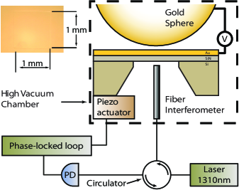
Figure 1: Schematic of the measurement apparatus. In the inset an optical image of the gold coated membrane is shown.

While approaching the sphere, the force experienced by the membrane has contributions from the Casimir Force as well as the electrostatic force. If we consider the first 3 terms of the Taylor expansion of the external force $F(z)$ about the distance $z_{0}$, the equation of motion of the nanomembrane becomes

$$\ddot{z}+2\gamma\dot{z}+\omega^{2}_{m}(z-z_{0}) = \frac{F_{d}(z_{0})}{m_{eff}}e^{i\omega_{d}t}+\frac{1}{m_{eff}}F^{\prime}(z_{0})(z-z_{0})$$ (1)

$$+\frac{1}{m_{eff}}\frac{F^{\prime\prime}(z_{0})}{2}(z-z_{0})^{2}$$

$$+\frac{1}{m_{eff}}\frac{F^{\prime\prime\prime}(z_{0})}{6}(z-z_{0})^{3}$$

where $\omega_{m}=2\pi f_{m}$ is the fundamental angular frequency of the membrane, $\omega_{d}$ the angular driving frequency, $\gamma$ is the damping coefficient, $F_{d}(z_{0})$ is the driving force, $m_{eff}$ the effective mass of the nanomembrane and $F^{\prime}$, $F^{\prime\prime}$, and $F^{\prime\prime\prime}$ are the derivatives of the external force with respect to the distance $z$. Although the resonator is set to operate in the linear regime there is some contribution from high order derivatives of the external force in the resonance frequency. The resonance frequency is modified by

$$\Delta f = -\frac{f_{m}}{2k_{eff}}\left(F^{\prime}(z_{0})+\frac{A^{2}_{\mathrm{rms}}}{6}F^{\prime\prime\prime}(z_{0})\right)$$ (2)

$$= -\frac{f_{m}}{2k_{eff}}F^{\prime}_{\mathrm{a}}(z_{0})$$

where $F^{\prime}_{\mathrm{a}}$ is the apparent force Lamoreaux (2010), $A_{\mathrm{rms}}$ the RMS amplitude of motion of the nanomembrane and $k_{eff}=m_{eff}{\omega_{0}}^{2}$ is the spring constant. The biggest contribution comes from the first derivative of the force Brown-Hayes et al. (2005) and the term with the third derivative of the force can be considered as a correction which is equivalent to the corrections for the roughness and the fluctuations of the plates that have been considered before Klimchitskaya et al. (1999); Sushkov et al. (2011).

We first evaluate the frequency resolution by measuring the frequency fluctuations of the resonators at a fixed membrane-sphere distance ($1\,\mathrm{\mu m}$). The Allan deviation is shown in Fig. 2, indicating that frequency resolution down to $2\cdot 10^{-9}$ can be achieved with integration time of $0.4\,\textrm{s}$. To achieve this resolution high stability of the resonance frequency is required, which is obtained by isolating the system from enviromental fluctuations. No ambient light is allowed to enter into the chamber to avoid thermal fluctuations. The temperature is stabilized within $0.1^{\circ}\textrm{C}$ and the granite table damps the external mechanical vibrations. This frequency resolution allows us to measure a force gradient of $3\,\mathrm{\mu N/m}$.

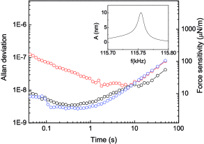
Figure 2: Left axis shows the Allan variance vs the integration time for several drive voltages: $500\,\mathrm{\mu V}$ (red), $10\,\mathrm{mV}$ (black), and $50\,\mathrm{mV}$ (blue). The right axis shows the equivalent gradient force sensitivity. The distance between the membrane and the sphere is $1\,\mathrm{\mu m}$. Inset, mechanical resonance $Q=14\,000$.

Having established high frequency resolution, we approach the sphere close to the membrane resonator utilizing the closed-loop piezoactuator. From Eq. (1) it can be found that the frequency shift can be fitted to a parabola Kim et al. (2009)

$$f^{2}=f_{0}(z)^{2}-K_{p}(z)(V-V_{m}(z))^{2}$$ (3)

where $V$ is the voltage applied between the membrane and the sphere. At each distance, a set of 3 voltages $V$ is applied Garcia-sanchez et al. . With these measurements we can find the fitting parameters: $f_{0}(z)$, $K_{p}(z)$ and $V_{m}(z)$. To improve the signal to noise ratio, the measurements are repeated approaching the sphere and retracting many times. $V_{m}$ represents the voltage that is required to minimize the electrostatic force given by the second term of the equation. It is worth emphasizing that the minimizing potential $V_{m}$ is not necessarily constant with the distance or the relative position between the membrane and the sphere because of the nonuniform work function or contact potential across the plate. It has been suggested that such a variation of $V_{m}$ can cause an additional electrostatic force Kim et al. (2010); Lamoreaux (2008). It can be found that $K_{p}(z)=\epsilon_{0}\pi Rf^{2}_{m}/k_{\mathrm{eff}}(z-z_{\mathrm{off}})^{2}$ where $R$ is the radius of the sphere, $z-z_{\mathrm{off}}$ the absolute distance, $z_{\mathrm{off}}$ the offset distance, $k_{\mathrm{eff}}$ the effective stiffness of the membrane and $\epsilon_{0}$ the vacuum permittivity. The parameters $k_{\mathrm{eff}}$ and $z_{\mathrm{off}}$ can be calculated by fitting the measured $K_{p}(z)$ to the expected model Kim et al. (2009). After calibration, for each measurement, the distance is calculated from the measured $K_{p}$ and the calibrated parameter $k_{\mathrm{eff}}$. We have estimated that the error in the position is about $1\,\mathrm{nm}$ at the closest distance. The measured stiffness $k_{\mathrm{eff}}$ is $4000\,\mathrm{N/m}$.

In Eq.(3), the first term $f_{0}^{2}$ has contributions from the Casimir force as well as from a residual electrostatic force that cannot be canceled, given by

$$\Delta f_{0}=-\frac{f_{m}}{2k_{\mathrm{eff}}}\left(\frac{dF_{c}(z)}{dz}+\frac{dF^{el}_{\mathrm{res}}(z)}{dz}\right)$$ (4)

where $F_{c}$ is the Casimir force and $F^{el}_{\mathrm{res}}(z)$ is the residual electrostatic force. By considering that the surface potentials are stochastic Kim et al. Kim et al. (2010) deduced a model for the residual electrostatic force as below:

$$F^{el}_{res}(z)=\pi R\epsilon_{0}[(V_{m}(z)+V_{1})^{2}+V^{2}_{\mathrm{rms}}]/z$$ (5)

where $V_{1}$ and $V_{\mathrm{rms}}$ are fitting parameters. $V_{\mathrm{rms}}$ accounts for the force originated by the patches that are smaller than the separation between the sphere and the plate.

The unambiguous measurement of the Casimir force also requires a mesurement of the surface contact potential distribution to ensure that the residual electrostatic force does not shield the Casimir force. Kelvin probe microscopes and its variations Robertson et al. (2006); Nonnenmacher et al. (1991); Kikukawa et al. (1995) have become reliable tools to inspect the contact potential difference (CPD) distribution of a surface.With our microscope we can also image the CPD between the sample and the sphere by scanning the sphere with respect to the membrane and simultaneously recording $V_{m}$. The CPD distribution is directly related to the spatial distribution of the patches on the sample. The patches on the sphere cannot be directly observed.

We show the results for two membranes on the same wafer, measured by the same sphere without breaking the vacuum. The first sample labeled “A” has large variations of the contact potential across the surface [see Figures 3a and 3c]. The variations of the contact potential depend on the relative position between the sphere and the nanomembrane in $x$, $y$ and $z$. Because of the nonuniform contact potential across the surface, the contact potential $V_{m}$ also largely depends on the distance between the sphere and the nanomembrane [see Fig. 3d]. These variations of the contact potential create an electric field between the sphere and the nanomembrane Kim et al. (2010). Because the energy of this field depends on the distance between the sphere and the membrane, there is a residual electrostatic force that appears. As mentioned above, this force can not be completely canceled by applying a voltage between the sphere and the nanomebrane Speake and Trenkel (2003); Kim et al. (2010). In Fig. 4a we show the contributions for this sample of the Casimir force and the residual electrostatic force. Because variations of the surface potential are large, the dominant force is electrostatic with the Casimir force a negligibly small fraction. The residual electrostatic force is well described by the model of Eq. (5) where $V_{\mathrm{rms}}=0.14\mathrm{V}$.

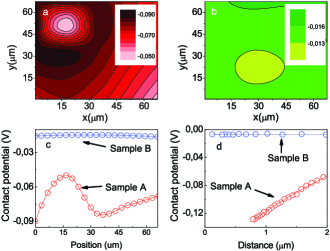
Figure 3: (a) Measured surface potential in volts of the sample A. The distance between the membrane and the sphere is $2\,\mathrm{\mu m}$. The data have been interpolated. (b) Measured surface potential in volts of the sample B. The distance between the membrane and the sphere is $0.15\,\mathrm{\mu m}$. At $2\,\mathrm{\mu m}$ the surface potential variations are too small to be resolved. (c) Line scan of surface potential at $y=50\,\mathrm{\mu m}$ for the samples A and B. (d) The contact potential $V_{m}$ for the samples A and B vs the distance with the sphere.

However, for the sample labeled “B” the spatial variation of the contact potential $V_{m}$ is very small [see Figs. 3b and 3c]. Because of the small variation of the surface contact potential, the variation of the contact potential with the distance is also small [see Fig. 3d]. These variations are small in comparison with the variations of the sample A. As a consequence, as shown in Fig. 4b the electrostatic force is negligible below $400\,\mathrm{nm}$, but it has to be taken into account above this distance and it is well described by the model of Eq. (5).

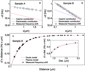
Figure 4: (a) The measured frequency of sample A is compared with the expected frequency due to the Casimir force and the residual electrostatic force. (b) The measured frequency of sample B is compared with the expected frequency due to the the casimir force and the residual electrostatic force. (c) The measured frequency for the sample B is compared with the expected frequency due to the Casimir force after correcting the contribution from the electrostatic patch for both the Drude and Plasma models. The inset shows a detail of the data. The error variance of the data have several origins such as the transducer noise and the precise determination of the distance between the sphere and the membrane.

Hence, because of the smaller electrostatic force, Sample B is employed for studying the Casimir force. The fluctuations of the position of the membrane have to be taken into account Vanbree et al. (1974); Lamoreaux (2005). The origin of these fluctuations are the roughness which is about $3\,\mathrm{nm}$ and the vibrations of the membrane which have an rms amplitude of $10\,\mathrm{nm}$. The correction that has to be applied to the Casimir force and the residual electrostatic force can be calculated from Eq. (2). Also the distance has to be corrected by a factor $\sqrt{1+\left(A_{\mathrm{rms}}/z\right)^{2}}$ because it has been extracted from the electrostatic force.

We further compare our measured results in sample B with the predictions from the Drude model Boström and Sernelius (2000) and the plasma model with the parameters $\omega_{p}=7.54\,\mathrm{eV}$ and $\gamma=0.051\,\mathrm{eV}$ Sushkov et al. (2011). With the Drude model, a least squares fit shows $V_{rms}=11.6\pm 0.2\,\mathrm{mV}$ with reduced $\chi^{2}$ (33 degrees of freedom) of 1.07 (probability to exceed 35%). On the other hand, a fit to the plasma model shows $V_{rms}=8.8\pm 0.5\,\mathrm{mV}$ with a reduced $\chi^{2}$ of 1.7 (probability to exceed 1%), suggesting that the Plasma model is ruled out to 99% confidence over this distance range. Figure 4c shows the measurements compared with the expected frequency shift due to the Casimir force after correcting the contribution from the electrostatic patch for both the Drude and Plasma models.

By employing high-Q nanomembranes with a force gradient sensitivity of $3\,\mathrm{\mu N}/\mathrm{m}$ we measured the Casimir force at $100\,\mathrm{nm}$-$2\,\mathrm{\mu m}$ separations. Our measurements show unambiguously that contact potentials play an important role in the precise measurement of the Casimir Force. By employing an in-situ surface potential measurements on our nanomembrane, we evaluate this uncertainty in measurements of the Casimir force. This reveals much scope for further improvements in accuracy by including methods to image such potentials on the sphere itself, which was not done in the measurements reported herein. Our data set indicates that the Drude model offers a better description of the mechanism in this range as compared to the plasma model.

This project was supported by DARPA/MTO’s Casimir Effect Enhancement project under SPAWAR contract no. N66001-09-1-2071. H. X. Tang acknowledges a Packard Fellowship in Science and Engineering and a CAREER Grant from National Science Foundation.

References

- Casimir (1948) H. B. G. Casimir, Proc. K. Ned. Akad. Wet. 51, 793 (1948).
- Boström and Sernelius (2000) M. Boström and B. E. Sernelius, Phys. Rev. Lett. 84, 4757 (2000).
- Brevik et al. (2005) I. Brevik, J. B. Aarseth, J. S. Høye, and K. A. Milton, Phys. Rev. E 71, 056101 (2005).
- Bezerra et al. (2004) V. B. Bezerra, G. L. Klimchitskaya, V. M. Mostepanenko, and C. Romero, Phys. Rev. A 69, 022119 (2004).
- Sushkov et al. (2011) A. O. Sushkov, W. J. Kim, D. A. R. Dalvit, and S. K. Lamoreaux, Nat Phys 7, 230 (2011).
- Decca et al. (2005) R. Decca, D. López, E. Fischbach, G. Klimchitskaya, D. Krause, and V. Mostepanenko, Annals of Physics 318, 37 (2005), special Issue.
- Bressi et al. (2002) G. Bressi, G. Carugno, R. Onofrio, and G. Ruoso, Phys. Rev. Lett. 88, 041804 (2002).
- Lamoreaux (1997) S. K. Lamoreaux, Phys. Rev. Lett. 78, 5 (1997).
- Mohideen and Roy (1998) U. Mohideen and A. Roy, Phys. Rev. Lett. 81, 4549 (1998).
- Chan et al. (2001a) H. B. Chan, V. A. Aksyuk, R. N. Kleiman, D. J. Bishop, and F. Capasso, Science 291, 1941 (2001a).
- Chan et al. (2001b) H. B. Chan, V. A. Aksyuk, R. N. Kleiman, D. J. Bishop, and F. Capasso, Phys. Rev. Lett. 87, 211801 (2001b).
- Kim et al. (2010) W. J. Kim, A. O. Sushkov, D. A. R. Dalvit, and S. K. Lamoreaux, Phys. Rev. A 81, 022505 (2010).
- Wilson-Rae et al. (2011) I. Wilson-Rae, R. A. Barton, S. S. Verbridge, D. R. Southworth, B. Ilic, H. G. Craighead, and J. M. Parpia, Phys. Rev. Lett. 106, 047205 (2011).
- (14) D. Garcia-sanchez, K. Y. Fong, H. Bhaskaran, S. Lamoreaux, and H. X. Tang, (To be published).
- (15) The sphere is a fused silica ball lens from Edmund Optics with ref. NT67-388.
- Lamoreaux (2010) S. K. Lamoreaux, Phys. Rev. A 82, 024102 (2010).
- Brown-Hayes et al. (2005) M. Brown-Hayes, D. A. R. Dalvit, F. D. Mazzitelli, W. J. Kim, and R. Onofrio, Phys. Rev. A 72, 052102 (2005).
- Klimchitskaya et al. (1999) G. L. Klimchitskaya, A. Roy, U. Mohideen, and V. M. Mostepanenko, Phys. Rev. A 60, 3487 (1999).
- Kim et al. (2009) W. J. Kim, A. O. Sushkov, D. A. R. Dalvit, and S. K. Lamoreaux, Phys. Rev. Lett. 103, 060401 (2009).
- Lamoreaux (2008) S. Lamoreaux, arXiv:0808.0885 (2008).
- Robertson et al. (2006) N. A. Robertson, J. R. Blackwood, S. Buchman, R. L. Byer, J. Camp, D. Gill, J. Hanson, S. Williams, and P. Zhou, Classical and Quantum Gravity 23, 2665 (2006).
- Nonnenmacher et al. (1991) M. Nonnenmacher, M. P. O’Boyle, and H. K. Wickramasinghe, Applied Physics Letters 58, 2921 (1991).
- Kikukawa et al. (1995) A. Kikukawa, S. Hosaka, and R. Imura, Applied Physics Letters 66, 3510 (1995).
- Speake and Trenkel (2003) C. C. Speake and C. Trenkel, Phys. Rev. Lett. 90, 160403 (2003).
- Vanbree et al. (1974) J. L. M. Vanbree, J. A. Poulis, B. J. Verhaar, and K. Schram, Physica 78, 187 (1974).
- Lamoreaux (2005) S. K. Lamoreaux, Reports on Progress in Physics 68, 201 (2005).