Neutron scattering experiments and simulations near the magnetic percolation threshold of $\rm{Fe}_{x}\rm{Zn}_{1-x}\rm{F}_{2}$

Abstract

The low temperature excitations in the anisotropic antiferromagnetic $\rm Fe_{1-x}Zn_{x}F_{2}$ for $x=0.25$ and $0.31$, at and just above the magnetic percolation threshold concentration $x_{\mathrm{p}}=0.25$, were measured using inelastic neutron scattering. The excitations were simulated for $x=0.31$ using a localized, classical excitation model, which accounts well for the energies and relative intensities of the excitations observed in the scattering experiments.

I INTRODUCTION

In two and three dimensions, spin wave excitations are well studied in pure isotropic and anisotropic insulating antiferromagnets Hutchings et al. (1970); Nikotin et al. (1969); Barak et al. (1978); Ikeda and Hutchings (1978); Windsor and Stevenson (1966). Magnetic excitations are significantly modified by magnetic dilution introduced by site substitution of the magnetic ions with diamagnetic ones. For isotropic systems near the magnetic percolation threshold concentration, $x_{\mathrm{p}}$, both well-resolved, local spin excitations as well as crossover from spin wave excitations to fracton excitations on a fractal-like lattice Itoh et al. (1998); Ikeda et al. (1998); Itoh et al. (2009, 2011); Ikeda et al. (1994); Nakayama et al. (1994), have been characterized near $x_{\mathrm{p}}$ in two and three dimensions. Local spin excitations have been observed in dilute two-dimensional anisotropic systems near $x_{\mathrm{p}}$ Ikeda and Ohoyama (1992). In three dimensions, magnetic excitations have been studied for the magnetically dilute anisotropic systems $\rm Mn_{0.5}Zn_{0.5}F_{2}$ Uemura and Birgeneau (1987) and $\rm Fe_{x}Zn_{1-x}F_{2}$ Paduani et al. (1994); Satooka et al. (2002); Rodriguez et al. (2007).

The parent compounds $\rm MnF_{2}$ and $\rm FeF_{2}$ exhibit comparable exchange energies and corresponding spin wave dispersions, but the $\rm FeF_{2}$ system has an order of magnitude larger anisotropy and a correspondingly larger spin wave gap. The excitations in the $\rm Mn_{0.5}Zn_{0.5}F_{2}$ system were interpreted in terms of spin wave to fracton crossover as the scattering wavevector $q$ increases. The behavior of the $\rm Fe_{x}Zn_{1-x}F_{2}$, for $x\geq 0.31$, has been interpreted Paduani et al. (1994) as showing both spin wave and local spin excitations for small $q$ and local spin excitations for large $q$. In this study, we examine magnetic excitations with high resolution neutron scattering experiments and computer simulations in $\rm Fe_{x}Zn_{1-x}F_{2}$ as $x$ approaches $x_{\mathrm{p}}=0.25$.

The well-characterized random-exchange antiferromagnet $\rm Fe_{x}Zn_{1-x}F_{2}$, with its simple structure and interactions, is an ideal anisotropic three-dimensional ($d=3$) system in which to study magnetic excitations through inelastic neutron scattering measurements and theoretical modeling and simulation. Magnetic excitations in the $d=3$ anisotropic antiferromagnet $\rm FeF_{2}$ have been very well characterized.Guggenheim et al. (1968); Hutchings et al. (1970) The structure of $\rm FeF_{2}$ and diamagnetic $\rm ZnF_{2}$ are similar.Stout and Reed (1954) The antiferromagnetic spins in $\rm FeF_{2}$ form a tetragonal lattice with two interpenetrating sublattices. The dominant antiferromagnetic inter-sublattice $J_{2}$ exchange interaction is between the body-center and body-corner magnetic ions. The intra-sublattice ferromagnetic $J_{1}$ and frustrating antiferromagnetic $J_{3}$ exchange interactions are much smaller (cf. Sec. III for further details). Best fit values from inelastic neutron scattering measurements are shown in Table I. $\rm FeF_{2}$ and diamagnetic $\rm ZnF_{2}$ mix well during crystal growth to form $\rm Fe_{x}Zn_{1-x}F_{2}$, which is a dilute, anisotropic, three-dimensional antiferromagnet. The occupation of sites by $\rm Fe^{2+}$ ions with $S=2$ or diamagnetic $\rm Zn^{2+}$ ions appears close to random, though slight clustering cannot be ruled out. It appears that $J_{2}$ does not vary significantly with dilution.King et al. (1981); de Araujo (1980) There is limited information about the effect of dilution on the anisotropy, but it also does not appear to vary by a large amount.de Araujo (1980)

Magnetic ordering in $\rm Fe_{x}Zn_{1-x}F_{2}$ has been experimentally studied previously Belanger et al. (1991); de Araujo et al. (1991); Paduani et al. (1994); Satooka and Ito (1997); Jonason et al. (1997); Barber and Belanger (2000); Satooka et al. (2002); Barbosa et al. (2003, 2005); Rodriguez et al. (2007); Belanger and Yoshizawa (1993); de Lima et al. (2012) at magnetic concentrations $x$ equal to or near $x_{\mathrm{p}}=0.246$, the magnetic percolation threshold for the body-centered tetragonal magnetic structure with an interaction between the body-centered and corner ions ($J_{2}$ in $\rm Fe_{x}Zn_{1-x}F_{2}$). The $H=0$ random-exchange transition should be expected for $x>x_{\mathrm{p}}$ if there is only the dominant exchange interaction $J_{2}$. However, the small $J_{1}$ and $J_{3}$ interactions in $\rm Fe_{x}Zn_{1-x}F_{2}$ could become influential near $x_{\mathrm{p}}$. The prior experiments in zero-field have demonstrated that for concentrations $x\leq 0.31$ Belanger et al. (1991) there is, at best, very weak long-range antiferromagnetic order at low temperatures. The system exhibits spin-glass-like behavior, dominated by slow dynamics near the percolation threshold, possibly a result of the frustrating $J_{3}$ interaction.

Early inelastic neutron scattering measurements in $\rm Fe_{x}Zn_{1-x}F_{2}$ were compared to a simple treatment with the excitation energies assigned Paduani et al. (1994) as $(z/n)E(q)$, where $n=8$ represents the number of neighbors in $\rm FeF_{2}$, $z\leq n$ is the possible number of neighbors of a given spin in the magnetically dilute system, and $E(q)$ is the spin wave energy as a function of the scattering wave vector $q$ in $\rm Fe_{x}Zn_{1-x}F_{2}$. The intensities are assigned by the combinatorial probabilities of finding $z$ neighbors of a given spin. While giving a fairly accurate description of the overall spread in energy, this description fails in the detailed structure of the excitation spectrum when higher energy resolution measurements resolve individual peaks. Similar results were found in far-infrared absorption experiments, high magnetic field pulsed laser absorption, and inelastic neutron scattering experiments for $x\geq 0.4$.Paduani et al. (1994); Satooka et al. (2002); Rodriguez et al. (2007) It was observed in the pulsed laser absorption measurements that the peaks become more easily resolvable for $x=0.4$ and that for this case the simplistic modeling described above proves wholly inadequate;Rodriguez et al. (2007) the spacings of the resolved peaks do not correspond to the simple model. The excitations were found to be largely localized, having little dispersion.

Here, we present a high resolution neutron-scattering study of $\rm Fe_{x}Zn_{1-x}F_{2}$ close to its percolation threshold. In agreement with the aforementioned work, the excitations show little or no dispersion. We show that a model of localized excitations accounts for our spectra even quantitatively.

The layout of the remaining part of this paper is as follows. In Sec. II, we report our new experimental results. The obtained spectra are rationalized through a simple model in Sec. III. Finally, we present our conclusions in Sec. IV.

II Experimental results

The results at $x=0.4$ motivated experiments closer to the percolation threshold and we have conducted inelastic neutron scattering studies for $x=0.25$ and $x=0.31$. Neutron scattering measurements were carried out using the high energy-resolution triple-axis spectrometer C1-1 installed at the JRR-3M reactor of JAEA in Tokai operating with a horizontally focusing analyzer with a final neutron energy of $E_{f}=3.1$ meV. The energy resolution at the elastic position is 0.09 meV (full width at half maximum) but it increases to 0.46 meV as the energy transfer increases to 8 meV. Single-crystal samples were mounted in a closed-cycle refrigerator with the c-axis perpendicular to the scattering plane. We examined a $\rm Fe_{0.25}Zn_{0.75}F_{2}$ single crystal with a mass of $2.24$g and a $\rm Fe_{0.31}Zn_{0.69}F_{2}$ single crystal with a mass of $1.72$g. The magnetic concentrations of the optical-quality crystals were determined using density measurements. The resulting scattering spectra of the experiments, shown in Figs. 1 and 2, indicate localized excitations since the excitation energies are largely independent of the scattering wave vector $q$. The simple approximation described above yields peaks similar to the resolved experimental peaks in the spectra, but the energies are not well predicted, as discussed below. It was clear that a more realistic calculation was needed to describe the peaks and to elucidate what governs the details of the $E$ vs $q$ spectra. We discuss simulations below that capture essential characteristics of the experimental results.

III Modeling the spectra

Figure 1: Experimental intensities vs energy for $x=0.25$ and $0.31$ for the zone center, $q=0$, for $q=0.25$, and for the zone boundary, $q=0.5$. The data for $x=0.25$ were taken at $T=0.7$K and those at $x=0.31$ were taken at $T=10$K. The curves are guides to the eye constructed from Gaussian peaks. The Gaussian peak locations are the same for each value of $q$. The ratio of intensities for $x=0.25$ and $x=0.31$ is arbitrary.

Figure 2: Experimental intensities vs energy for $x=0.25$ at $T=0.7$, $20$, and $40$K to show the temperature dependence of the neutron scattering spectra.

We have remarked in the previous section that, to a large extent, the scattering spectra are independent of the scattering wave vector, which suggests that the underlying excitations are spatially localized and therefore can be described by a local model. Local spin Hamiltonians for pure $\rm{Fe}\rm{F}_{2}$ have been extensively discussed,Guggenheim et al. (1968); Hutchings et al. (1970, 1972) and include both an on-site interaction characterized by an anisotropy parameter $D$, and Heisenberg exchange interactions characterized by three coupling constants $J_{1}$, $J_{2}$ and $J_{3}$. The strongest exchange is the antiferromagnetic $J_{2}$ that couples nearest neighbors belonging to different sublattices of the body-centered tetragonal magnetic lattice of $\rm{Fe}$ atoms, while $J_{1}$ and $J_{3}$ couple atoms belonging to the same sublattice, i.e., bonds parallel to the edges of the unit cell (Fig. 3).

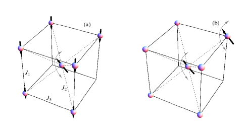
Figure 3: (a) Unit cell with seven occupied sites of which the central site is active and the six dimmed sites are held frozen in an antiferromagnetic configuration. (b) The same unit cell with all the occupied sites being active (for clarity, only two of them are marked with flipping arrows). The corresponding frozen environment is the next shell of neighbors (not shown in the figure).

Following the same pattern, we model the disordered sample with the following Hamiltonian:

$$H = -D\sum_{i}\epsilon_{i}\big{[}S_{i}^{(z)}\big{]}^{2}+J_{2}\sum_{\langle i,j\rangle}\epsilon_{i}\epsilon_{j}{\boldsymbol{S}}_{i}\cdot{\boldsymbol{S}}_{j}$$ (1)

$${}+J_{1}\sum_{\langle\langle i,j\rangle\rangle}\epsilon_{i}\epsilon_{j}{\boldsymbol{S}}_{i}\cdot{\boldsymbol{S}}_{j}+J_{3}\sum_{\langle\langle\langle i,j\rangle\rangle\rangle}\epsilon_{i}\epsilon_{j}{\boldsymbol{S}}_{i}\cdot{\boldsymbol{S}}_{j},$$

where the ${\boldsymbol{S}}_{i}$ are $S=2$ spin operators that represent the $\rm{Fe}$ atoms, and where the substitutional disorder is represented by statistically independent random variables $\epsilon_{i}$ which take the value one with probability $x$ (the fraction of $\rm{Fe}$ atoms) and the value zero with probability $1-x$ (the fraction of nonmagnetic $\rm{Zn}$ atoms symbolized as empty sites in Fig. 3).

Table 1: Best fit parameters, taken from Ref. Hutchings et al., 1970, for the spin Hamiltonian of pure $\rm{Fe}\rm{F}_{2}$.

$D(\rm{cm}^{-1})$	$J_{1}(\rm{cm}^{-1})$	$J_{2}(\rm{cm}^{-1})$	$J_{3}(\rm{cm}^{-1})$
$6.46(+0.29,-0.10)$	$-0.048\pm 0.060$	$3.64\pm 0.10$	$0.194\pm 0.060$

Table 1 shows the parameters obtained by Hutchings et al. Hutchings et al. (1970) by fitting inelastic neutron scattering data of $\rm{Fe}\rm{F}_{2}$ to the spin Hamiltonian, and it is often assumed that the same values can be used for the analysis of the dilute antiferromagnet Paduani et al. (1994); Satooka et al. (2002) (we will elaborate on this point later). The fact that $|J_{1}|,J_{3}\ll J_{2}<D$ allows us to get an estimate of the spectrum at low temperatures by ignoring in the Hamiltonian (1) the terms proportional to $J_{1}$ and $J_{3}$ and making the approximation ${\boldsymbol{S}}_{i}\cdot{\boldsymbol{S}}_{j}\approx S_{i}^{(z)}S_{j}^{(z)}$ in the terms proportional to $J_{2}$. For the sake of definiteness let us consider a site $i$ on the A sublattice, with $n_{2}$ $\rm{Fe}$ neighbors (the probability distribution function for $n_{2}=0,1,\ldots,8$ is binomial). Since at very low temperatures the magnetic state of the sample is essentially the Néel state ($S_{i}^{(z)}=+2$ if the site $i$ belongs to the A sublattice and $S_{i}^{(z)}=-2$ if $i$ is in the B sublattice), the local magnetic field felt by the spin $i$ due to the $n_{2}$ surrounding atoms is $-2n_{2}J_{2}$. Hence, the contribution of spin $i$ to the energy is $E_{i}=-D[S_{i}^{(z)}\big{]}^{2}-2n_{2}J_{2}S_{i}^{(z)}$. An incoming neutron typically causes a spin flip $S_{i}^{(z)}=2\rightarrow S_{i}^{(z)}=1$; the energy of such a transition is

$$\Delta E\approx 3D+2n_{2}J_{2},$$ (2)

and therefore to a first approximation the spectrum consists of nine evenly spaced zero-width peaks with a binomial distribution of intensities. The anisotropy parameter $D$ determines the average position of the peaks, while the spacing between peaks is proportional to $J_{2}$. Actually, a more accurate description can be obtained by averaging the immediate generalization of Eq. (2)

$$\Delta E\approx 3D-2n_{1}J_{1}+2n_{2}J_{2}-2n_{3}J_{3},$$ (3)

over the respective number of neighboring sites $0\leq n_{1}\leq 2$, $0\leq n_{2}\leq 8$, $0\leq n_{3}\leq 4$. In Fig. 4 we show the result of this calculation with the parameters of the pure sample Hutchings et al. (1970) and (zero-width) intensities proportional to the products of the respective combinatorial weights. This figure shows how the coupling constants $J_{1}$ and $J_{3}$ contribute to the effective spread of the peaks. In fact, comparison with the fit to the experimental data suggests that all the pure sample parameters need to be modified to describe the highly diluted sample and, in particular, that the anisotropy parameter $D$ is too large. As we will see in the forthcoming discussion, the parameters that provide the best fit to the experimental data depend on the approximation scheme used to study the model Eq. (1). However, the semiclassical picture given by Eq. (3) and illustrated in Fig. 4 remains qualitatively correct in the full simulation.

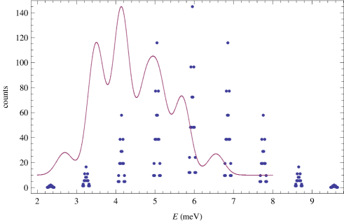
Figure 4: Semiclassical approximation to the spectrum provided by Eq. (3) averaged over the respective number of neighboring sites with the pure sample parameters. Hutchings et al. (1970) The solid line is a fit to the experimental data of Fig. 1 corresponding to $x=0.31$ and $q=0.5$, and suggests that the pure sample parameters need to be modified to describe the highly diluted sample.

Our approach to simulate the experimental spectra is a two-step procedure. In the first step we use the full Hamiltonian (1) but maintain the approximation ${\boldsymbol{S}}_{i}\cdot{\boldsymbol{S}}_{j}\approx S_{i}^{(z)}S_{j}^{(z)}$ for the exchange terms, so that we can generate typical local environments by a classical Monte Carlo simulation. More concretely, we generate equilibrium spin configurations at $T=10~{}\rm{K}$ using a heat bath combined with a cluster method in lattices with $2\times 32^{3}$ sites with an $\rm{Fe}$ density $x=0.31$. After we equilibrate ten such lattices (samples) we pick at random on each sample 1000 nonempty sites. We call this site, together with its $n$ nearest neighbors, as illustrated in Fig. 3(b), a dynamic shell, and the next shell of atoms [not shown in Fig. 3(b)], the local environment. Figure 3(a) illustrates a simpler version of this idea, in which there is only one spin in the dynamic shell (the central spin marked by a flipping arrow) and there are six frozen atoms in an antiferromagnetic state that constitute the local environment.

In the second step of our procedure we use the full Hamiltonian (1) with full quantum spin operators for each atom on the dynamic shell, while the nondynamic spins that constitute the local environment are kept fixed and act in effect as boundary conditions for the dynamic shell. Since the third component of the total spin for each dynamic shell

$$S^{(z)}=\sum_{i\ \text{dynamic}}S_{i}^{(z)}$$ (4)

commutes with the Hamiltonian, we find the ground state (G.S.) within the subspace corresponding to the Néel state $S^{(z)}=S_{\text{N\'{e}el}}$, which amounts to diagonalizing a square matrix with up to $3000$ states, and the excited states by diagonalizing the Hamiltonian restricted to the subspaces $S^{(z)}=S_{\text{N\'{e}el}}\pm 1$ allowed by the selection rules. The transition energies are simply the energy differences

$$\Delta E^{\pm}_{k}=E_{k}^{S_{\text{N\'{e}el}}\pm 1}-E_{\text{G.S.}}^{S_{\text{N\'{e}el}}}.$$ (5)

The exact calculation of the intensities in this experimental setting involves the matrix elements of a rather complicated interaction Hamiltonian.Moon et al. (1969) We settle for an estimate of the relative intensities of these transitions and consider the simplest possible interaction operator (in fact, one of the terms appearing in the full expression), which is proportional to $S_{i}^{(\pm)}$, where $i$ denotes the central atom of the dynamic shell. The contribution of each transition (5) to the total intensity is proportional to

$$|\langle k,S^{(z)}=S_{\text{N\'{e}el}}\pm 1|S_{i}^{(\pm)}|\text{G.S.},S^{(z)}=S_{\text{N\'{e}el}}\rangle|^{2}.$$ (6)

We have found that the main effect of the simplified transition matrix element (6) is to suppress the contributions of high-energy transitions. Note also that the combinatorial factor is already included in our sampling of the simulation results. Finally, we add up the contributions of all the possible transitions in our 1000 samples, calculate the convolution of this result with the measured instrumental resolution function (a Gaussian with moderate energy-dependent width), and normalize the result to match the maximum count of the experimental curves (it would seem better to match the integrated intensity in the experimental range, but as we will see, the resulting widths are too narrow).

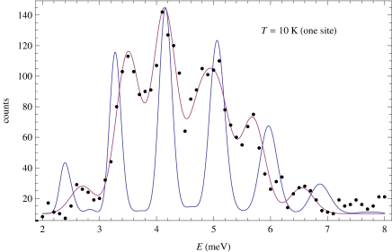
Figure 5: Experimental data for $q=0.5$, numerical fitting and simulated spectrum at $T=10~{}\rm{K}$ with the parameters of the pure sample Hutchings et al. (1970) for: (a) a one-site calculation corresponding to the dynamic shell of Fig. 3(a); (b) calculation corresponding to the dynamic shell of Fig. 3(b).

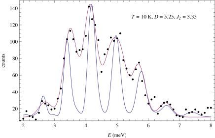
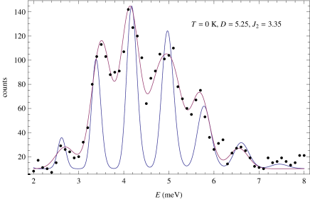
Figure 6: Experimental points, numerical fitting and simulated spectrum with fitted values of $D$ and $J_{2}$ corresponding to the dynamic shell of Fig. 3(b) for: (a) $T=10~{}\rm{K}$; (b) $T=0~{}\rm{K}$ (i.e., purely antiferromagnetic environment).

Figure 5 shows the results of these procedures for the two dynamic shells illustrated in Fig. 3 in the energy range between $2~{}\rm{meV}$ and $8~{}\rm{meV}$. The figures show the experimental points, a numerical fitting to these points, and our simulation results. The one-site calculation reproduces quite well the main features of the experimental spectrum, including the average position of the peaks (controlled by the anisotropy parameter $D$), although the separation between peaks (controlled by the coupling constant $J_{2}$) is too large and, as we anticipated, the widths are too narrow.

Although the simulation results corresponding to the dynamic shell of Fig. 3(b) feature wider widths, the average position is clearly shifted to high energies, which suggests that, not only the value of $J_{2}$, but also the value of the anisotropy parameter $D$ may be too large in this context. A possible explanation might be related to the method by which the pure sample parameters Hutchings et al. (1970) are obtained, whereby a semiclassical approximation is used to determine the spectrum parametrically as a function of $D$, $J_{1}$, $J_{2}$ and $J_{3}$, and later these parameters are fitted to match the experimental results. In essence, this procedure involves a calculation to first order in $1/S$, which should give better results for $S\gg 1$ i.e., for the one-site approximation. This possibility has already been noticed. For example, in Ref. Paduani et al., 1994 certain empirical relations between the parameters of the pure of the diluted sample are proposed.

Following these ideas, in Fig. 6(a) we show the result of an optimization of the parameters $J_{2}$ and $D$ to match the experimental results, which yielded $J_{2}=3.35~{}\text{cm}^{-1}$ and $D=5.25~{}\text{cm}^{-1}$. Unfortunately, the correlation between these parameters and the uncertainties prevents a more accurate determination of these values or the simultaneous optimization of the less significant $J_{1}$ and $J_{3}$ that we have kept fixed. Although the widths of the peaks are still too narrow, the intensities are quite well accounted for, and even a last peak at $E\approx 7.4~{}\text{meV}$ seems to be reproduced.

Finally, as an estimate of the thermal effects in our simulations, in Fig. 6(b) we show a similar calculation at $T=0~{}\rm{K}$, i.e., with a purely antiferromagnetic state (no thermal disorder) of the environment. Note the distinctly narrower widths and poorer intensity relations between the peaks, particularly at high energies.

There are a variety of possible reasons to explain the larger experimental widths: our scattering operator is oversimplified, as it does not take into account the relative orientation of the lattice and the wave vector of the incoming neutron, which we also assume perfectly well defined (i.e., we neglect the spread of the neutron beam); the dynamic shells and their environments have been obtained from a classical (rather than quantum) Monte Carlo, which surely overestimates the spin ordering at low temperatures; and the dynamic shells are limited to spins and their immediate neighbors.

IV Discussion

In summary, we have presented high-resolution spectra from neutron scattering experiments, conducted over $\rm{Fe}_{x}\rm{Zn}_{1-x}\rm{F}_{2}$ close to its percolation threshold. We model these spectra in terms of a site diluted Heisenberg model, containing both ferromagnetic and antiferromagnetic exchange interactions. In spite of its simplicity and with only a moderate adjustment of the parameters, the proposed model accounts quite well for the position and intensity relations of the peaks in the spectra. This success is probably due to the validity of our main hypothesis, namely the local nature of the spin excitations in these systems which lie close to the percolation threshold for the $\rm{Fe}$ lattice.

Whereas local spin excitations dominate the energy spectrum for $x$ near $x_{\mathrm{p}}$ in $\rm Fe_{1-x}Zn_{x}F_{2}$, we cannot rule out a very small contribution from fracton excitations in a similar energy range. Fracton excitations as well as local spin excitations coexist in isotropic systems and both may exist in the small anisotropy $\rm Mn_{1-x}Zn_{x}F_{2}$ system as $x$ approaches $x_{\mathrm{p}}$. In that case, modeling the local spin excitations could aid in separating the two types of excitations, allowing the characterization of local spin excitations as well as the persistence of fracton excitations under conditions of weak anisotropy.

Acknowledgments

We acknowledge partial financial support from MICINN, Spain, (Grant Nos. FIS2009-12648-C03 and FIS2011-22566), and from UCM-Banco Santander (GR32/10-A/910383, GR58/08-910556). V.M.-M. thanks the del Amo foundation and the hospitality of the Physics Department of U. California-Santa Cruz, where part of this work was performed. We thank the members of the Neutron Scattering Laboratory, Institute for Solid State Physics, the University of Tokyo for supporting our experiments.

References

- Hutchings et al. (1970) M. T. Hutchings, B. D. Rainford, and H. J. Guggenheim, J. Phys. C 3, 307 (1970).
- Nikotin et al. (1969) O. Nikotin, P. A. Lindgard, and O. W. Dietrich, J. Phys. C: Sol. State Phys. 2, 1168 (1969).
- Barak et al. (1978) J. Barak, V. Jaccarino, and S. M. Rezende, J. Magn. Magn. Mater. 9, 323 (1978).
- Ikeda and Hutchings (1978) H. Ikeda and M. T. Hutchings, J. Phys. C: Solid State Phys. 11, L529 (1978).
- Windsor and Stevenson (1966) C. G. Windsor and R. W. H. Stevenson, Proc. Phys. Soc. 87, 501 (1966).
- Itoh et al. (1998) S. Itoh, H. Ikeda, H. Yoshizawa, M. J. Harris, and U. Steigenberger, J. Phys. Soc. Jpn. 67, 3610 (1998).
- Ikeda et al. (1998) H. Ikeda, M. Takahashi, J. A. Fernandez-Baca, and R. M. Nicklow, J. Magn. Magn. Mater. 177-181, 139 (1998).
- Itoh et al. (2009) S. Itoh, T. Nakayama, R. Kajimoto, and M. A. Adams, J. Phys. Soc. Jpn. 78, 013707 (2009).
- Itoh et al. (2011) S. Itoh, T. Nakayama, and M. A. Adams, J. Phys. Soc. Jpn. 80, 104704 (2011).
- Ikeda et al. (1994) H. Ikeda, J. A. Fernandez-Baca, R. M. Nicklow, M. Takahashi, and K. Iwasa, J. Phys. Cond. Matter 6, 10543 (1994).
- Nakayama et al. (1994) T. Nakayama, K. Yakubo, and R. L. Orbach, Rev. Mod. Phys. 66, 381 (1994).
- Ikeda and Ohoyama (1992) H. Ikeda and K. Ohoyama, Phys. Rev. B 45, 7484 (1992).
- Uemura and Birgeneau (1987) Y. J. Uemura and R. J. Birgeneau, Phys. Rev. B 36, 7024 (1987).
- Paduani et al. (1994) C. Paduani, D. P. Belanger, J. Wang, S. J. Han, and R. M. Nicklow, Phys. Rev. B 50, 193 (1994).
- Satooka et al. (2002) J. Satooka, K. Katsumata, and D. P. Belanger, J. Phys.: Condens. Matter 14, 1307 (2002).
- Rodriguez et al. (2007) Y. W. Rodriguez, I. E. Anderson, D. P. Belanger, H. Nojiri, F. Ye, and J. A. Fernandez-Baca, J. Magn. Magn. Mater. 310, 1546 (2007).
- Guggenheim et al. (1968) H. J. Guggenheim, M. T. Hutchings, and B. D. Rainford, J. Appl. Phys. 39, 1120 (1968).
- Stout and Reed (1954) J. W. Stout and S. A. Reed, J. Am. Chem. Soc. 76, 5279 (1954).
- King et al. (1981) A. R. King, V. Jaccarino, T. Sakakibara, M. Motokawa, and M. Date, Phys. Rev. Lett. 47, 117 (1981).
- de Araujo (1980) C. B. de Araujo, Phys. Rev. B 22, 266 (1980).
- Belanger et al. (1991) D. P. Belanger, W. E. Murray, F. C. Montenegro, A. R. King, V. Jaccarino, and R. W. Erwin, Phys. Rev. B 44, 2161 (1991).
- de Araujo et al. (1991) J. H. de Araujo, J. B. M. da Cunha, A. Vasquez, L. Amaral, J. T. Moro, F. C. Montenegro, S. M. Rezende, and M. D. Coutinho-Filho, Hyper. Inter. 67, 507 (1991).
- Satooka and Ito (1997) J. Satooka and A. Ito, J. Phys. Soc. Jpn. 66, 784 (1997).
- Jonason et al. (1997) K. Jonason, C. Djurberg, P. Nordblad, and D. P. Belanger, Phys. Rev. B 56, 5404 (1997).
- Barber and Belanger (2000) W. C. Barber and D. P. Belanger, Phys. Rev. B 61, 8960 (2000).
- Barbosa et al. (2003) P. H. R. Barbosa, E. P. Raposo, and M. D. Coutinho-Filho, Phys. Rev. Lett. 91, 197207 (2003).
- Barbosa et al. (2005) P. H. R. Barbosa, E. P. Raposo, and M. D. Coutinho-Filho, Phys. Rev. B 72, 092401 (2005).
- Belanger and Yoshizawa (1993) D. P. Belanger and H. Yoshizawa, Phys. Rev. B 47, 5051 (1993).
- de Lima et al. (2012) K. A. P. de Lima, J. B. Brito, P. H. R. Barbosa, E. P. Raposo, and M. D. Coutinho-Filho, Phys. Rev. B 85, 064416 (2012).
- Hutchings et al. (1972) M. T. Hutchings, M. P. Schulhof, and H. J. Guggenheim, Phys. Rev. B 5, 154 (1972).
- Moon et al. (1969) R. M. Moon, T. Riste, and W. C. Koehler, Phys. Rev. 181, 920 (1969).