Seismic probes of solar interior magnetic structure

Abstract

Sunspots are prominent manifestations of solar magnetoconvection and imaging their subsurface structure is an outstanding problem of wide physical importance. Travel times of seismic waves that propagate through these structures are typically used as inputs to inversions. Despite the presence of strongly anisotropic magnetic waveguides, these measurements have always been interpreted in terms of changes to isotropic wavespeeds and flow-advection related Doppler shifts. Here, we employ PDE-constrained optimization to determine the appropriate parameterization of the structural properties of the magnetic interior. Seven different wavespeeds fully characterize helioseismic wave propagation: the isotropic sound speed, a Doppler-shifting flow-advection velocity and an anisotropic magnetic velocity. The structure of magnetic media is sensed by magnetoacoustic slow and fast modes and Alfvén waves, each of which propagates at a different wavespeed. We show that even in the case of weak magnetic fields, significant errors may be incurred if these anisotropies are not accounted for in inversions. Translation invariance is demonstrably lost. These developments render plausible the accurate seismic imaging of magnetoconvection in the Sun.

Sunspots are substantial deviations from the quiet Sun, with umbral temperatures dropping by as much as 20% from ambient conditions. Numerous questions swirl around sunspot physics, such as understanding their long-time stability (compared to convective turnover timescales) and appreciating their creation, emergence and eventual death. The use of helioseismic waves to probe the structure of sunspots has a long and controversial history (for a review, see, e.g., Gizon et al. (2010)). Inversions for sunspot sub-surface structure and dynamics (e.g., Kosovichev and Duvall (1997)) attempt to explain away the observed effects on seismic waves by an entirely isotropic wavespeed, an approximation that has faced subsequent marginalization (e.g., Gizon et al. (2009)) owing to the widespread recognition of strong anisotropies prevalent in sunspots. Forward modeling of wave propagation in sunspots has generated a deeper appreciation for measurements and fully realistic non-linear sunspot evolution calculations (Rempel et al. (2009)) have proven successful. However, posing an inverse problem that accounts for these anisotropies remains an outstanding problem of great relevance, towards whose eventual resolution this article takes a significant step.

Waves are excited stochastically in the Sun due to the action of vigorous near-surface convection. The cross correlation of wavefield velocities measured at the photosphere of the Sun (by measuring Doppler shifts of absorption lines formed at the photosphere; e.g., the Helioseismic and Magnetic Imager onboard the Solar Dynamics Observatory Schou et al. (2012)) is empirically known to be an ergodic random process (e.g., Gizon and Birch (2004)). The associated travel time of a wave between two points on the solar photosphere is estimated by fitting the cross correlation of the plasma velocities measured at those points. We introduce a misfit functional, defined as the $L_{2}$ norm of the difference between observed ($\tau_{i}^{\mathrm{o}}$) and predicted ($\tau_{i}^{\mathrm{p}}$) travel times along a collection of paths $i$: $\sum_{i}(\tau_{i}^{\mathrm{o}}-\tau_{i}^{\mathrm{p}})^{2}$. We then pose the following PDE-constrained optimization problem

$$\chi=\sum_{i}(\tau_{i}^{\mathrm{o}}-\tau_{i}^{\mathrm{p}})^{2}-\int_{\odot}d{\bf x}\int d\omega\,{\boldsymbol{\lambda}}\cdot({\boldsymbol{\mathcal{L}}}{\boldsymbol{\xi}}-{\bf S}),$$ (1)

where $\chi$ is the cost function, ${\bf S}$ the wave source, $\omega$ temporal frequency, ${\bf x}$ the spatial coordinate and ${\boldsymbol{\lambda}}({\bf x},\omega)$ a vector Lagrange multiplier, the dual to the wave displacement ${\boldsymbol{\xi}}({\bf x},\omega)$. The predicted travel times are linear functionals of wave displacement ${\boldsymbol{\xi}}$. The helioseismic wave operator ${\boldsymbol{\mathcal{L}}}$ comprises temporally stationary model properties, which we attempt to determine. We reproduce it here in the temporal-frequency domain (e.g., Hanasoge et al. (2011)),

$${\boldsymbol{\mathcal{L}}}{\boldsymbol{\xi}}=-\omega^{2}\rho{\boldsymbol{\xi}}-i\omega\rho\Gamma{\boldsymbol{\xi}}-2i\omega\rho{\bf v}\cdot{\boldsymbol{\nabla}}{\boldsymbol{\xi}}$$ (2)

$$-{\boldsymbol{\nabla}}(c^{2}\rho{\boldsymbol{\nabla}}\cdot{\boldsymbol{\xi}})-{\boldsymbol{\nabla}}({\boldsymbol{\xi}}\cdot{\boldsymbol{\nabla}}p)+{\bf g}{\boldsymbol{\nabla}}\cdot(\rho{\boldsymbol{\xi}})$$

$$-\frac{1}{4\pi}({\boldsymbol{\nabla}}{\boldsymbol{\times}}{\bf B}){\boldsymbol{\times}}[{\boldsymbol{\nabla}}{\boldsymbol{\times}}({\boldsymbol{\xi}}{\boldsymbol{\times}}{\bf B})]-\frac{1}{4\pi}\{{\boldsymbol{\nabla}}{\boldsymbol{\times}}[{\boldsymbol{\nabla}}{\boldsymbol{\times}}({\boldsymbol{\xi}}{\boldsymbol{\times}}{\bf B})]\}{\boldsymbol{\times}}{\bf B},$$

where the properties of interest are the density $\rho$, sound speed $c$, vector magnetic field ${\bf B}$ and flows ${\bf v}$. Wave damping is denoted by $\Gamma$ and gravity by ${\bf g}$, where these are held fixed and not considered to be parameters here, the justifications for which may be found in Hanasoge et al. (2011). Acceleration, wave damping, and Doppler shifting by flow advection are the first two terms of operator (2), the isotropic wavespeed term and buoyancy terms form the second line and the final two terms are due to the anisotropic Lorentz force. Background pressure $p$ is constrained by the magneto-hydrostatic (MHS) equilibrium equation

$${\boldsymbol{\nabla}}p=-\rho{\bf g}+{\boldsymbol{\nabla}}\cdot\left({\bf B}{\bf B}-\frac{{\bf B}\cdot{\bf B}}{2}\,{\bf I}\right),$$ (3)

where ${\bf I}$ is the identity tensor. Two scalar thermal parameters, density and sound speed, and two vector quantities, flows and magnetic fields, are the independent variables that we invert for and pressure is constrained by equation (3).

Given wave operator (2), we study in detail the variation of the cost function (1) to obtain the gradients of the travel-time misfit functional with respect to model parameters (e.g., Tromp et al. (2010); Hanasoge et al. (2011)). These gradients, also known as sensitivity kernels or Fréchet derivatives, are indicators of information in the seismic wavefield and their sensitivity to relevant model parameters. The computational realization of this method (Tromp et al. (2010); Hanasoge et al. (2011)) for two-point correlation function measurements, as in the Sun, requires calculating a predictive so-called forward wavefield and an adjoint wavefield that assimilates the misfit. Sensitivity kernels for various physical quantities (which form the corrector) emerge from a temporal convolution of these two wave fields, allowing us to pose an inverse problem of the form

$$\delta\chi=-\int_{\odot}d{\bf x}\,K_{c}\,\delta c+{\bf K}_{\bf v}\cdot\delta{\bf v}+{\bf K}_{\bf B}\cdot\delta{\bf B}+K^{\prime}_{\rho}\,\delta\ln\rho,$$ (4)

where $K_{c},{\bf K}_{\bf v},{\bf K}_{\bf B}$ are sensitivity kernels for sound speed, flows and magnetic fields, while ${K}^{\prime}_{\rho}$ the kernel for density, termed as an impedance kernel in geophysics jargon, is sensitive to reflectors (e.g., Zhu et al. (2009)). Equation (4) states that the measured travel-time shift comprises a sum of volume integrals of these perturbations weighted by the corresponding finite-frequency wave sensitivities. Travel times are very weakly sensitive to density variations but record sharp contrasts in impedance, such as (possibly) the horizontal boundary of a sunspot. We do not expect to be able to image such reflections since the wavelength of waves that we consider are large in comparison to possible rapid variations, but retain and compute these kernels in any case (see Figures 2 and 4 of supplemental material).

A critical aspect to setting up an inverse problem is in appreciating the physical variables to which waves are sensitive. It is seen that the variation of the operator (2) has terms (among others) that contain $\rho\,\delta c^{2},\rho\,\delta{\bf v}$ and $\delta{\bf B}$ (see also detailed expressions for kernels in Hanasoge et al. (2011)). This immediately tells us that kernels for sound speed and flows are weighted by the density of the model, in contrast to kernels for the primitive magnetic field. Further, variables $c$ and ${\bf v}$ are forms of wavespeed, which suggests the use of Alfvén velocity, ${\bf a}={\bf B}/\sqrt{4\pi\rho}$ instead of the primitive ${\bf B}$ field. One may conceive of it as a descriptor of the anisotropic wave velocity to which waves are directly sensitive. Straightforward manipulation allows us to rewrite the kernels as follows

$$\delta{\bf B}=\delta({\bf a}\sqrt{4\pi\rho})=\sqrt{4\pi\rho}\,\delta{\bf a}+\frac{1}{2}{\bf a}\sqrt{4\pi\rho}\,\delta\ln\rho,$$ (5)

which together with equation (4) gives

$$\sqrt{4\pi\rho}\,{\bf K}_{\bf B}={\bf K}_{\bf a}\,\,\,\,\,\,\,\,\,\,\,\,K^{\prime}_{\rho}\rightarrow K^{\prime}_{\rho}+\frac{1}{2}{\bf K}_{\bf a}\cdot{\bf a},$$ (6)

thus providing a new expression for variations in the misfit

$$\delta\chi=-\int_{\odot}d{\bf x}\,K_{c}\,\delta c+{\bf K}_{\bf v}\cdot\delta{\bf v}+{\bf K}_{\bf a}\cdot\delta{\bf a}+K^{\prime}_{\rho}\,\delta\ln\rho.$$ (7)

We note that the first three terms represent three types of wavespeeds, an isotropic sound speed, an advection related flow velocity and lastly, an intrinsically anistropic velocity. Although not shown here, weighting the magnetic field kernels by the square-root of density redistributes incoherent sensitivity from the upper-most atmospheric layers to the photosphere and shallow interior. The transformation for the density kernel in equation (5) now contains a contribution from the Alfvén velocity, and could in principle be used to image reflections off sharp velocity contrasts.

The single-scattering first-Born approximation cannot capture the full scope of wave propagation in strong perturbations such as sunspots (i.e., with respect to the quiet Sun; e.g., Gizon et al. (2006)). This implies that inversions for the sub-surface structure of sunspots are likely to require an iterative algorithm, since we have to sequentially refine the predicted travel times, which are nonlinearly related to changes in the model. Thus, in the analysis here, we construct a ‘sunspot’ in MHS equilibrium (Eq. [3]) and determine sensitivity kernels relative to this model.

We introduce a 2-D stream function $\psi(x,z)$ such that the magnetic field is given by ${\bf B}=(-\partial_{z}\psi,\partial_{x}\psi)$. Since ${\bf g}=(0,-g)$, Lorentz forces in the $x$ direction are solely balanced by the pressure gradient in equation (3), i.e., $\partial_{x}p=\partial_{x}(B_{x}^{2}/2-B_{z}^{2}/2)+\partial_{z}(B_{x}B_{z})$. From this equation we calculate the pressure distribution required to support this field configuration and then use the $z$ component of equation (3) to obtain the associated density. Generating an MHS state is non trivial since density and pressure decrease exponentially as a function of height above the photosphere; consequently, a large range of choices for the field configuration results in negative pressures or densities or both. Field configurations with strong horizontal and vertical fields also require the action of flows to maintain force balance, an aspect we do not consider here because the complexity of such a model renders difficult the interpretation of the attendant kernels. We show one example field configuration in Figure 1.

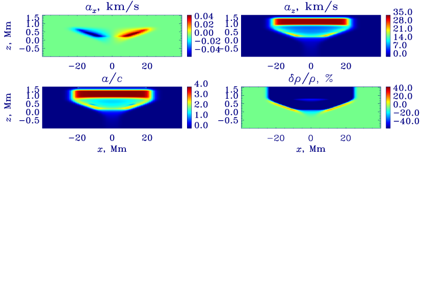
Figure 1: Magnetic field configuration in our calculations. Top panels show Aflvén speeds $a_{x}=B_{x}/\sqrt{4\pi\rho}$ and $a_{z}=B_{z}/\sqrt{4\pi\rho}$, which are signed quantities. The bottom left panel is the ratio of the absolute Alfvén speed to the local sound speed and is seen to be on the order of 1 at the photosphere. The field is relatively weak with the highest Alfvén speed around 35 km/s and a Wilson depression of 250 km. (for an expanded view, see Figure 1 of the supplemental material)

A major difficulty in simulating wave propagation through strong magnetic fields is that Alfvén speed $||{{\bf a}}||$ becomes extremely large in the atmospheric layers of the Sun (due to the exponentially rapidly decreasing density), resulting in a very stiff differential equation. Further, wave travel times are very weakly sensitive to the dynamics of these layers because the modes are trapped below the photosphere. A multiplicative prefactor is introduced to control the amplitude of the Lorentz force terms in (2), (e.g., Cameron et al. (2008); Rempel et al. (2009)). However, this method results in a model that is not seismically reciprocal (e.g., Hanasoge et al. (2011)), a central requirement in the formal interpretation of helioseismic measurements and the determination of sensitivity kernels. Here, in order to maintain seismic reciprocity while still saturating the Alfvén speed at 40 km/s, we directly multiply the magnetic field by a prefactor. While this results in a background field configuration that has a non-zero divergence, we note that small-amplitude oscillations about this field are still divergence free. Further, in the scheme of linear inversions for magnetic structure, the divergence-free nature of the background field is not a strict requirement but could be considered a regularization term.

We perform linear magneto-hydrodynamic (MHD) wave propagation simulations in Cartesian geometry, using the pseudo-spectral code SPARC (Hanasoge and Duvall (2007); Hanasoge et al. (2008); Hanasoge (2008)). Horizontal derivatives are computed using Fast Fourier Transforms, vertical derivatives are estimated on a non-uniform grid using compact finite differences (Lele (1992)) and time-stepping is effected through the repeated application of an optimized Runge-Kutta scheme (Hu et al. (1996)). Vertical boundaries are lined with absorbent convolutional perfectly matched layers (Hanasoge et al. (2010)) that are designed to absorb MHD waves as well. We implement a phenomenological wave damping term along the lines of the recipe suggested by Schunker et al. (2011). Because we restrict ourselves to a 2-D field configuration in this problem, Aflvén waves are disallowed and only magneto-acoustic fast and slow waves propagate.

We focus here on the diagnostic ability of the surface $f$ and acoustic $p_{1}$ modes, so chosen because of their significant sensitivity to surface layers. The measurement consists of ridge filters applied to isolate these modes. The sunspot is assumed to be located at disk center, implying that the line-of-sight component is co-aligned with the (vertical) $z$ axis. Thus the vertical wavefield displacement is used to define the cross correlation measurement. We show the power spectra and cross correlations in Figure 2. We employ the linear travel-time definition (Gizon and Birch (2002, 2004)), also used previously by Hanasoge et al. (2011) to estimate travel time shifts from cross correlations.

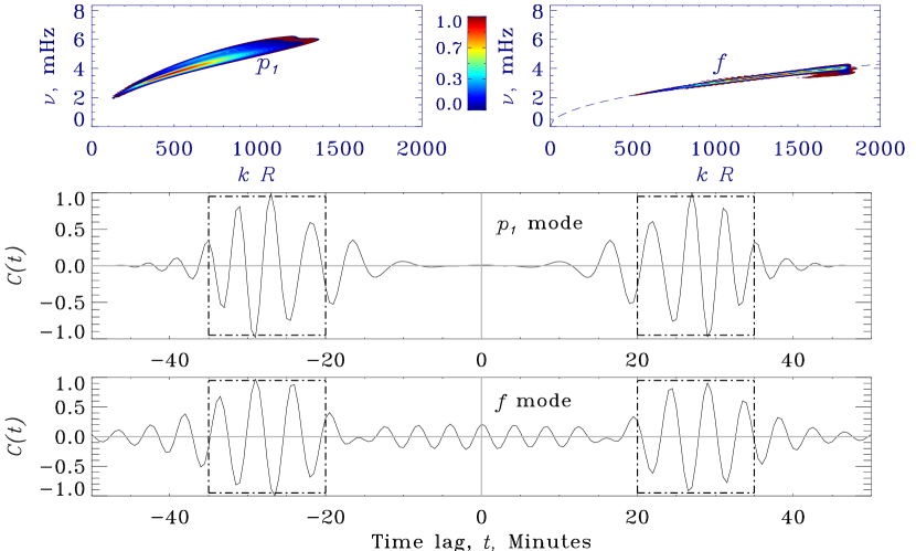
Figure 2: Expectation value of the power spectrum of the $p_{1}$ and $f$ ridge-filtered measurements (top panels). The limit cross correlation ${\mathcal{C}}(t)$ between a point 15 Mm from the left of the sunspot center to a point 10 Mm on the right of the center is shown for the $p_{1}$ measurement (middle panel). The $f$-mode cross correlation is between the center of the sunspot and a point 10 Mm to the right (bottom panel). See Figures 3 and 4 also. The positive-time branch is sensitive to waves that first arrive at one measurement point and subsequently at the other and vice versa. The loss of translational variance implies that the absolute locations of the points matter. The dot-dash boxes indicate the measurement windows. Travel time shifts of waves are obtained by estimating the deviation of the cross correlation from a reference wavelet. Mean travel times, defined as the average of the time shifts of oppositely traveling waves, are thought to be largely sensitive to structure. Difference travel times, defined as the difference between the shifts, are considered primarily sensitive to symmetry-breaking flows. (for an expanded view, see Figure 2 of the supplemental material)

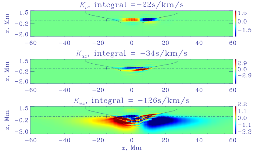
Figure 3: $f$-mode (surface) wavespeed kernels for a difference travel-time measurement between a point-pair 10 Mm apart. Kernels sensitive to isotropic sound speed, Alfvén speed $a_{x}$ and vertical flows $v_{z}$ are shown. The boundary of the spot, marked by the solid black line, is much smaller than the horizontal wavelength. The horizontal dot-dash line denotes the height at which observations are made in the quiet Sun and the symbols mark the measurement points. The $f$-mode is seen to be significantly affected by the spot, as seen in the loss in symmetry of the kernels. Signatures of magneto-acoustic slow and fast modes and hints of conversion to acoustic $p_{1}$ may be plausibly discerned upon examination. The integrals of the kernels show that the travel times are significantly affected by the presence of even this relatively weak magnetic field. (for an expanded view, see Figure 3 of the supplemental material)

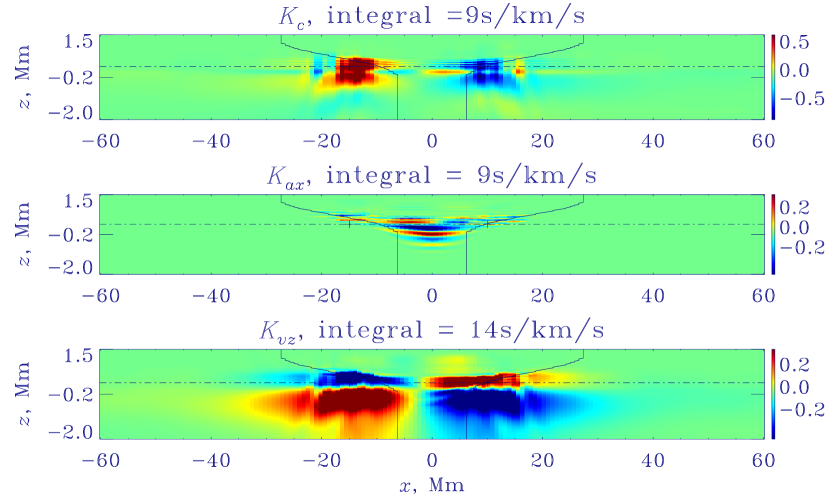
Figure 4: $p_{1}$-mode wavespeed kernels for a difference travel-time measurement between a point-pair 25 Mm apart. The panels from top to bottom show kernels sensitive to sound speed (top), Alfvén speeds $a_{x}$ and vertical flows $v_{z}$. The boundary of the spot, marked by the solid black line, is much smaller than the horizontal wavelength. The horizontal dot-dash line denotes the height at which observations are made in the quiet Sun and the symbols mark the measurement points. Plausible signatures of slow modes propagating down into the tube may be discerned in the middle panel. (for an expanded view, see Figure 4 of the supplemental material)

Figure 3 (see also Figures 5 and 6 in the supplemental material) displays the sensitivity of the surface $f$-mode to the sunspot. Because we model waves as finite spatial objects, their sensitivities extend beyond just the ray path. It can be seen that the effect of the spot is significant in that the kernels are noticeably asymmetric between the point-pair. The time shifts induced by the magnetic field are considerable, comparable in magnitude to those induced by flow and thermal perturbations. There are hints of mode conversion from $f$ to $p_{1}$ in the difference kernel for sound speed (top), just below the pixel on the right.

In Figure 4 (see also Figures 7 and 8 in the supplemental material), we show a set of difference $p_{1}$-mode kernels for a point pair separated by a distance of 25 Mm respectively. Because the magnetic field is relatively weak compared to a sunspot, the acoustic $p_{1}$ mode, whose energy is focused in the sub-surface layers, is much less affected by the field than the $f$ mode. Symmetry is nearly completely restored to the $p_{1}$ kernels.

The Alfvén speed kernels for both $f$ and $p_{1}$ modes show features of high spatial frequency, and contain signatures of fast and slow magneto-acoustic waves. In the umbral regions of the sunspot, waves of high spatial frequency are seen to be propagating toward the interior (plausibly slow waves).

Our computations support the view that inversions for sunspots, especially when using surface modes, are greatly over-simplified if anisotropic wave speeds are not taken into account. The realization of this method has required a number of theoretical and numerical advances, paving the way for seismic imaging of magneto-convection in the solar interior.

Acknowledgements. All calculations were run on the Pleiades supercomputer at NASA ARC. S. M. H. acknowledges support from NASA grant NNX11AB63G.

References

- Gizon et al. (2010) L. Gizon, A. C. Birch, and H. C. Spruit, Ann. Rev. of Astronomy and Astrophysics 48, 289 (2010).
- Kosovichev and Duvall (1997) A. G. Kosovichev and T. L. Duvall, Jr., in SCORe’96 : Solar Convection and Oscillations and their Relationship, Astrophysics and Space Science Library, Vol. 225, edited by F. P. Pijpers, J. Christensen-Dalsgaard, and C. S. Rosenthal (1997) pp. 241–260.
- Gizon et al. (2009) L. Gizon et al., Space Science Reviews 144, 249 (2009).
- Rempel et al. (2009) M. Rempel, M. Schüssler, and M. Knölker, Astrophys. J. 691, 640 (2009).
- Schou et al. (2012) J. Schou et al., Solar Physics 275, 229 (2012).
- Gizon and Birch (2004) L. Gizon and A. C. Birch, Astrophys. J. 614, 472 (2004).
- Hanasoge et al. (2011) S. M. Hanasoge, A. Birch, L. Gizon, and J. Tromp, Astrophys. J. 738, 100 (2011).
- Tromp et al. (2010) J. Tromp, Y. Luo, S. Hanasoge, and D. Peter, Geophysical Journal International 183, 791 (2010).
- Zhu et al. (2009) H. Zhu, Y. Luo, T. Nissen-Meyer, C. Morency, and J. Tromp, Geophysics 74, 167 (2009).
- Gizon et al. (2006) L. Gizon, S. M. Hanasoge, and A. C. Birch, Astrophys. J. 643, 549 (2006).
- Cameron et al. (2008) R. Cameron, L. Gizon, and T. L. Duvall, Jr., Solar Physics 251, 291 (2008).
- Hanasoge and Duvall (2007) S. M. Hanasoge and T. L. Duvall, Jr., Astronomische Nachrichten 328, 319 (2007).
- Hanasoge et al. (2008) S. M. Hanasoge, S. Couvidat, S. P. Rajaguru, and A. C. Birch, Monthly Notices of the Royal Astronomical Society 391, 1931 (2008).
- Hanasoge (2008) S. M. Hanasoge, Astrophys. J. 680, 1457 (2008).
- Lele (1992) S. K. Lele, Journal of Computational Physics 103, 16 (1992).
- Hu et al. (1996) F. Q. Hu, M. Y. Hussaini, and J. L. Manthey, Journal of Computational Physics 124, 177 (1996).
- Hanasoge et al. (2010) S. M. Hanasoge, D. Komatitsch, and L. Gizon, Astronomy & Astrophysics 522, A87 (2010).
- Schunker et al. (2011) H. Schunker, R. H. Cameron, L. Gizon, and H. Moradi, Solar Physics 271, 1 (2011).
- Gizon and Birch (2002) L. Gizon and A. C. Birch, Astrophys. J. 571, 966 (2002).