Noncolliding Brownian Motion with Drift and Time-Dependent Stieltjes-Wigert Determinantal Point Process

Abstract

Using the determinantal formula of Biane, Bougerol, and O’Connell, we give multitime joint probability densities to the noncolliding Brownian motion with drift, where the number of particles is finite. We study a special case such that the initial positions of particles are equidistant with a period $a$ and the values of drift coefficients are well-ordered with a scale $\sigma$. We show that, at each time $t>0$, the single-time probability density of particle system is exactly transformed to the biorthogonal Stieltjes-Wigert matrix model in the Chern-Simons theory introduced by Dolivet and Tierz. Here one-parameter extensions ($\theta$-extensions) of the Stieltjes-Wigert polynomials, which are themselves $q$-extensions of the Hermite polynomials, play an essential role. The two parameters $a$ and $\sigma$ of the process combined with time $t$ are mapped to the parameters $q$ and $\theta$ of the biorthogonal polynomials. By the transformation of normalization factor of our probability density, the partition function of the Chern-Simons matrix model is readily obtained. We study the determinantal structure of the matrix model and prove that, at each time $t>0$, the present noncolliding Brownian motion with drift is a determinantal point process, in the sense that any correlation function is given by a determinant governed by a single integral kernel called the correlation kernel. Using the obtained correlation kernel, we study time evolution of the noncolliding Brownian motion with drift.

I Introduction

Vicious walker models on lattices Fis84 and their continuum versions Dys62 , which will be called noncolliding diffusion processes KT07 ; KT_Sugaku_11 , have been extensively studied in connection with the random matrix theory NF98 ; FNH99 ; Gra99 ; Baik00 ; Joh02 ; NF02 ; KT02 ; NKT03 ; KT04 ; KT10 , the Tracy-Widom distributions and extreme value statistics TW94 ; TW96 ; TW04 ; TW07 ; KIK08a ; SMCR08 ; KIK08b ; FMS11 ; Lie12 , the enumerative combinatorics and representation theory GOV98 ; KGV00 ; ABE10 ; Fei12 ; ABE12 , the Riemann-Hilbert problem KMW09 ; DKZ11 ; KMW11 , the renormalization group theory CK03 ; GG10a ; GG10b , the growth models PS02 ; Joh03 ; IS05 , the quantum integrable systems Kat11 ; OCo12a ; Kat12a , and others. Construction of noncolliding diffusion processes has been based on the determinantal formula for nonintersecting paths of Karlin-McGregor (KM) KM59 and Lindström-Gessel-Viennot (LGV) Lin73 ; GV85 . It can be regarded as a stochastic version of Slater’s determinantal wave function for free fermions in quantum mechanics and it means that indistinguishability of particles (i.e. invariance of statistics under any exchange of paths at intersecting points on the spatio-temporal plane) should be assumed. In general, if each walker (diffusion particle) has different drift, then they are distinguishable from each other and the KM-LGV determinantal formula is not applicable.

If the values of drift coefficients of many particles are well-ordered, however, Biane, Bougerol and O’Connell BBO05 proved that the following determinantal formula is valid. Let $N=2,3,\dots$, and we consider an $N$-particle system of Brownian motions in the one-dimensional real space $\mathbb{R}$ such that the $j$-th Brownian particle starts at $x_{j}\in\mathbb{R}$ at time $t=0$ and it has a constant drift $\nu_{j}$ per time, $1\leq j\leq N$. In other words, we consider an $N$-dimensional vector-valued diffusion process

$$\mbox{\boldmath$B$}^{\mbox{\boldmath$x$},\mbox{\boldmath$\nu$}}(t)=\mbox{\boldmath$B$}^{\mbox{\boldmath$x$}}(t)+\mbox{\boldmath$\nu$}t,\quad t\geq 0,$$ (1)

whose $j$-th component describes the $j$-th Brownian motion with a drift coefficient $\nu_{j}$,

$$B^{x_{j},\nu_{j}}_{j}(t) = B^{x_{j}}_{j}(t)+\nu_{j}t$$ (2)

$$= x_{j}+B_{j}(t)+\nu_{j}t,\quad t\geq 0,\quad 1\leq j\leq N,$$

where $B_{j}(t),t\geq 0,1\leq j\leq N$, are independent one-dimensional standard Brownian motions all started at the origin. Let

$$\mathbb{W}_{N}=\{\mbox{\boldmath$x$}=(x_{1},x_{2},\dots,x_{N})\in\mathbb{R}^{N}:x_{1}<x_{2}<\cdots<x_{N}\},$$ (3)

which is called the Weyl chamber of type A_N-1 in the representation theory FH91 . Biane, Bougerol and O’Connell (BBO) showed that BBO05 , if the values of the components of initial configuration $\mbox{\boldmath$x$}=(x_{1},x_{2},\dots,x_{N})$ and the drift vector $\mbox{\boldmath$\nu$}=(\nu_{1},\nu_{2},\dots,\nu_{N})$ are in the same order, that is,

$$\mbox{\boldmath$x$}\in\mathbb{W}_{N},\quad\mbox{\boldmath$\nu$}\in\mathbb{W}_{N},$$ (4)

then the transition probability density of the drifted Brownian motions (1) conditioned never to collide with each other is given by

$$p_{N}^{\mbox{\boldmath$\nu$}}(t,\mbox{\boldmath$y$}|\mbox{\boldmath$x$})=e^{-t|\mbox{\boldmath$\nu$}|^{2}/2}\frac{\displaystyle{\det_{1\leq j,k\leq N}[e^{\nu_{j}y_{k}}]}}{\displaystyle{\det_{1\leq j,k\leq N}[e^{\nu_{j}x_{k}}]}}q_{N}(t,\mbox{\boldmath$y$}|\mbox{\boldmath$x$}),\quad\mbox{\boldmath$y$}\in\mathbb{W}_{N},\quad t\geq 0,$$ (5)

where $|\mbox{\boldmath$\nu$}|^{2}=\sum_{j=1}^{N}\nu_{j}^{2}$ and

$$q_{N}(t,\mbox{\boldmath$y$}|\mbox{\boldmath$x$})=\det_{1\leq j,k\leq N}\Big{[}p(t,y_{j}|x_{k})\Big{]}$$ (6)

with the transition probability density of $B(t)$,

$$p(t,y|x)=\frac{1}{\sqrt{2\pi t}}e^{-(y-x)^{2}/2t},\quad t\geq 0.$$ (7)

(We give a brief review of the BBO argument BBO05 in Appendix A.)

In the formula (5), we note that even when some of $\nu_{j}$’s in $\mbox{\boldmath$\nu$}=(\nu_{1},\dots,\nu_{N})$ coincide, the ratio of determinants $\det_{1\leq j,k\leq N}[e^{\nu_{j}y_{k}}]/\det_{1\leq j,k\leq N}[e^{\nu_{j}x_{k}}]$ can be interpreted using l’Hôpital’s rule. In particular, if we take the limit $\nu_{j}\to 0,1\leq j\leq N$, (5) is reduced to be

$$p_{N}(t,\mbox{\boldmath$y$}|\mbox{\boldmath$x$})=\frac{h_{N}(\mbox{\boldmath$y$})}{h_{N}(\mbox{\boldmath$x$})}q_{N}(t,\mbox{\boldmath$y$}|\mbox{\boldmath$x$}),\quad\mbox{\boldmath$y$}\in\mathbb{W}_{N},\quad t\geq 0$$ (8)

with the Vandermonde determinant

$$h_{N}(\mbox{\boldmath$x$})=\det_{1\leq j,k\leq N}[x_{j}^{k-1}]=\prod_{1\leq j<k\leq N}(x_{k}-x_{j}).$$ (9)

It is considered as Doob’s harmonic transform ($h$-transform) KT_Sugaku_11 of the KM-LGV determinant $q_{N}(t,\mbox{\boldmath$y$}|\mbox{\boldmath$x$})$ by $h_{N}$, in which $h_{N}$ is harmonic in the sense that $\Delta h_{N}(\mbox{\boldmath$x$})\equiv\sum_{j=1}^{N}\partial^{2}h_{N}(\mbox{\boldmath$x$})/\partial x_{j}^{2}=0$. The above observation implies that the BBO formula (5) is a generalization of the $h$-transform of KM-LGV determinant (8).

In (8), we can take the limit $x_{j}\to 0,1\leq j\leq N$, which is denoted by $\mbox{\boldmath$x$}\to{\bf 0}$, and we obtain the probability density of particle positions $\mbox{\boldmath$y$}=(y_{1},y_{2},\dots,y_{N})$ of the noncolliding Brownian motions all started at the origin,

$$p_{N}(t,\mbox{\boldmath$y$}|{\bf 0})=c_{N}(t)(h_{N}(\mbox{\boldmath$y$}))^{2}e^{-|\mbox{\boldmath$y$}|^{2}/2t},\quad\mbox{\boldmath$y$}\in\mathbb{W}_{N},\quad t\geq 0$$ (10)

with $c_{N}(t)=t^{-N^{2}}/\{(2\pi)^{N/2}\prod_{j=1}^{N}\Gamma(j)\}$. The important fact is that (10) can be identified with the probability density of eigenvalues of random matrices (ordered in $\mathbb{W}_{N}$) in the Gaussian unitary ensemble (GUE) with variance $\sigma^{2}=t$ Meh04 ; For10 . When $\mbox{\boldmath$x$}\not={\bf 0}$, (8) gives the probability density of eigenvalues $\{y_{j}\}_{j=1}^{N}$ in the GOE-GUE two-matrix model studied in the high-energy physics Meh04 , in which the hermitian random matrix is coupled with a real-symmetric random matrix with eigenvalues $\{x_{j}\}_{j=1}^{N}$ KT02 ; Kat12_pf . In this sense, the BBO formula (5) is expected to be related with some matrix-models which are generalizations of two-matrix models. (See BBO05 ; BBO09 ; OCo12b for the relations of (5) with the Duistermaat-Heckman measure and the Littelmann path model in representation theory.)

On the other hand, the BBO formula (5) is regarded as a simplified version of the transition probability density of the O’Connell process, which is a stochastic version of the quantum Toda lattice OCo12a . The reduction from the O’Connell process to the noncolliding Brownian motion with drift is called a combinatorial limit (or tropicalization) and the inverse procedure is called a geometric lifting BBO09 ; OCo12b ; Kat12b ; Kat12c . (See Appendix B.) In an earlier paper Kat12b , we took the limit $\mbox{\boldmath$x$}\to{\bf 0}$ with keeping $\mbox{\boldmath$\nu$}\in\mathbb{W}_{N}$ and derived a reciprocal time relation between the noncolliding Brownian motion with drift $\nu$ started at ${\bf 0}$ and that without drift started at a configuration given by $\nu$. We would like to say that the BBO formula (5) is located in the high level in the random matrix theory and it also gives an introduction to mathematical models in higher levels OCo12b ; BC11 ; Kat12c .

In the present paper, we consider a special case such that the drift coefficients and initial positions are given by the following. Let $n\in\mathbb{N}\equiv\{1,2,\dots,\},N=2n-1$ and define

$$\rho = \left(-\frac{N-1}{2},-\frac{N-1}{2}+1,\dots,-1,0,1\dots,\frac{N-1}{2}-1,\frac{N-1}{2}\right)$$ (11)

$$= (-n+1,-n+2,\cdots,n-2,n-1).$$

Then we put

$$x_{j}=a\rho_{j}=a(j-n)=a\left(j-\frac{N+1}{2}\right),\quad 1\leq j\leq N,$$ (12)

$$\nu_{j}=\sigma\rho_{j}=\sigma(j-n)=\sigma\left(j-\frac{N+1}{2}\right),\quad 1\leq j\leq N,$$ (13)

with positive constants $a>0,\sigma>0$. Although this setting seems to be very special, we find that the obtained process can be transformed to a matrix model in Chern-Simons theory recently introduced by Dolivet and Tierz DT07 . Precisely speaking, the normalization factor of the single-time probability density in our process gives the inverse of partition function $Z$ of their matrix model. Since here we study an interacting particle system (the noncolliding Brownian motion with drift) we can discuss not only the partition function but also correlation functions. Dolivet and Tierz shows that the ensemble of eigenvalues of their matrix model realizes the biorthogonal ensemble Mut95 ; Bor99 associated with the one-parameter extension DT07 of the Stieltjes-Wigert polynomials Sze81 ; KS96 . As an extension of their result, we will show in this paper that this ensemble is a determinantal (fermion) point process in the sense of Sos00 ; ST03 . This implies that, at each time $t>0$, the noncolliding Brownian motion started at the equidistant points (12) with the special drift (13) is also a determinantal point process, whose correlation kernel is expressed by using the biorthogonal Stieltjes-Wigert polynomials. We will report the time-evolution of the correlation functions of this noncolliding Brownian motion with drift.

The paper is organized as follows. The probability densities of the noncolliding Brownian motion with drift and its transformations are given in Sec.II. The biorthogonal Stieltjes-Wigert polynomials are introduced in Sec.III and determinantal structure of the ensembles are studied there. In Sec.IV the main result is stated and analytic and numerical study of time-evolution of the present noncolliding Brownian motion with drift using the correlation kernel is reported. Concluding remarks will be given in Sec.V. Appendices are prepared for the BBO argument, the O’Connell process, and the geometric Brownian motions, which are related with the present process.

II Probability Densities of the Particle Systems

II.1 Multitime Joint Probability Density of the Noncolliding Brownian Motion with Drift

In a previous paper Kat12b , we considered an $N$-particle system of noncolliding Brownian motion started at $\mbox{\boldmath$x$}=(x_{1},x_{2},\cdots,x_{N})\in\overline{\mathbb{W}}_{N}\equiv\{\mbox{\boldmath$x$}\in\mathbb{R}^{N}:x_{1}\leq x_{2}\leq\cdots\leq x_{N}\}$ with a drift vector $\mbox{\boldmath$\nu$}=(\nu_{1},\nu_{2},\dots,\nu_{N})$ satisfying $\mbox{\boldmath$\nu$}\in\overline{\mathbb{W}}_{N}$. For any $M\in\mathbb{N}$ and an arbitrary $M$ sequence of times $0<t_{1}<t_{2}<\cdots<t_{M}<\infty$, the multitime joint probability density of the process is given by

$$p_{N}^{\mbox{\boldmath$\nu$}}(t_{1},\mbox{\boldmath$x$}^{(1)};\dots;t_{M},\mbox{\boldmath$x$}^{(M)}|\mbox{\boldmath$x$})$$

$$=e^{-t_{M}|\mbox{\boldmath$\nu$}|^{2}/2}\det_{1\leq j,k\leq N}\left[e^{\nu_{j}x^{(M)}_{k}}\right]\prod_{m=1}^{M-1}q_{N}(t_{m+1}-t_{m},\mbox{\boldmath$x$}^{(m+1)}|\mbox{\boldmath$x$}^{(m)})\frac{q_{N}(t_{1},\mbox{\boldmath$x$}^{(1)}|\mbox{\boldmath$x$})}{\displaystyle{\det_{1\leq j,k\leq N}[e^{\nu_{j}x_{k}}]}},$$ (14)

where particle configurations at each time $t_{m}$ is denoted by $\mbox{\boldmath$x$}^{(m)}=(x^{(m)}_{1},\dots,x^{(m)}_{N})\in\mathbb{W}_{N},1\leq m\leq M$. Here $q_{N}$ is the KM-LGV determinant given by (6). From this general formula, we can obtain the following multitime joint probability density for the special case (12) and (13).

Proposition 1  Consider the noncolliding Brownian motion with $N$ particles started at the equidistant points (12) at time $t=0$ with the drift having the coefficients (13). For an arbitrary $M\in\mathbb{N}$ and an arbitrary sequence of times $0<t_{1}<t_{2}<\cdots<t_{M}<\infty$, the multitime joint probability density of the process is given by

$$\widehat{p}_{N}(t_{1},\mbox{\boldmath$x$}^{(1)};\dots;t_{M},\mbox{\boldmath$x$}^{(M)})=c_{N}(a,\sigma,t_{1},t_{M})\prod_{\ell=1}^{N}(e^{\sigma x^{(M)}_{\ell}})^{-(N-1)/2}$$

$$\quad\quad\times\prod_{1\leq j<k\leq N}(e^{\sigma x^{(M)}_{k}}-e^{\sigma x^{(M)}_{j}})\prod_{m=1}^{M-1}q_{N}(t_{m+1}-t_{m},\mbox{\boldmath$x$}^{(m+1)}|\mbox{\boldmath$x$}^{(m)})$$

$$\quad\quad\times\prod_{j=1}^{N}p(t_{1},x^{(1)}_{j}|0)\prod_{\ell=1}^{N}(e^{ax^{(1)}_{\ell}/t_{1}})^{-(N-1)/2}\prod_{1\leq j<k\leq N}(e^{ax^{(1)}_{k}/t_{1}}-e^{ax^{(1)}_{j}/t_{1}})$$ (15)

with

$$c_{N}(a,\sigma,t_{1},t_{M})=\frac{1}{\prod_{n=1}^{N-1}(e^{na\sigma}-1)^{N-n}}\exp\left\{-\frac{1}{24}N(N^{2}-1)\left(\sigma^{2}t_{M}-2a\sigma+\frac{a^{2}}{t_{1}}\right)\right\}.$$ (16)

It is also written as

$$\widehat{p}_{N}(t_{1},\mbox{\boldmath$x$}^{(1)};\dots;t_{M},\mbox{\boldmath$x$}^{(M)})$$

$$=c_{N}(a,\sigma,t_{1},t_{M})\prod_{1\leq j<k\leq N}\left[2\sinh\frac{\sigma(x^{(M)}_{k}-x^{(M)}_{j})}{2}\right]\prod_{m=1}^{M-1}q_{N}(t_{m+1}-t_{m},\mbox{\boldmath$x$}^{(m+1)}|\mbox{\boldmath$x$}^{(m)})$$

$$\qquad\qquad\times\prod_{j=1}^{N}p(t_{1},x^{(1)}_{j}|0)\prod_{1\leq j<k\leq N}\left[2\sinh\frac{a(x^{(1)}_{k}-x^{(1)}_{j})}{2t_{1}}\right].$$ (17)

Proof   If we set the drift vector as (13) with a positive constant $\sigma>0$, we obtain

$$\det_{1\leq j,k\leq N}[e^{\nu_{j}x_{k}}]=\det_{1\leq j,k\leq N}\Big{[}(e^{\sigma x_{k}})^{j-1-(N-1)/2}\Big{]}=\prod_{\ell=1}^{N}(e^{\sigma x_{\ell}})^{-(N-1)/2}\prod_{1\leq j<k\leq N}(e^{\sigma x_{k}}-e^{\sigma x_{j}}).$$

We find that the above is equal to

$$\prod_{1\leq j<k\leq N}\left[2\sinh\frac{\sigma(x_{k}-x_{j})}{2}\right].$$

Note that

$$|\mbox{\boldmath$\nu$}|^{2}=\sigma^{2}|\mbox{\boldmath$\rho$}|^{2}=\sigma^{2}\sum_{j=1}^{N}\left(j-\frac{N+1}{2}\right)^{2}=\frac{1}{12}N(N^{2}-1)\sigma^{2}.$$

Then the multitime joint probability density of the process with drift coefficients (13) is given by

$$p_{N}^{\sigma\mbox{\boldmath$\rho$}}(t_{1},\xi^{(1)};\dots;t_{M},\xi^{(M)}|\mbox{\boldmath$x$})$$

$$\quad=e^{-N(N^{2}-1)\sigma^{2}t_{M}/24}\prod_{\ell=1}^{N}(e^{\sigma x^{(M)}_{\ell}})^{-(N-1)/2}\prod_{1\leq j<k\leq N}(e^{\sigma x^{(M)}_{k}}-e^{\sigma x^{(M)}_{j}})$$

$$\qquad\times\prod_{m=1}^{M-1}q_{N}(t_{m+1}-t_{m},\mbox{\boldmath$x$}^{(m+1)}|\mbox{\boldmath$x$}^{(m)})\frac{q_{N}(t_{1},\mbox{\boldmath$x$}^{(1)}|\mbox{\boldmath$x$})}{\displaystyle{\prod_{\ell=1}^{N}(e^{\sigma x_{\ell}})^{-(N-1)/2}\prod_{1\leq j<k\leq N}(e^{\sigma x_{k}}-e^{\sigma x_{j}})}}$$

$$\quad=e^{-N(N^{2}-1)\sigma^{2}t_{M}/24}\prod_{1\leq j<k\leq N}\left[2\sinh\frac{\sigma(x^{(M)}_{k}-x^{(M)}_{j})}{2}\right]$$

$$\qquad\times\prod_{m=1}^{M-1}q_{N}(t_{m+1}-t_{m},\mbox{\boldmath$x$}^{(m+1)}|\mbox{\boldmath$x$}^{(m)})\frac{q_{N}(t_{1},\mbox{\boldmath$x$}^{(1)}|\mbox{\boldmath$x$})}{\displaystyle{\prod_{1\leq j<k\leq N}\left[2\sinh\frac{\sigma(x_{k}-x_{j})}{2}\right]}}.$$ (18)

Then we assume that the initial configuration is given by the equidistant points (12) with $a>0$. We can see that in this setting

$$q_{N}(t_{1},\mbox{\boldmath$x$}^{(1)}|a\mbox{\boldmath$\rho$})$$

$$\quad=e^{-N(N^{2}-1)a^{2}/24t_{1}}\frac{e^{-|\mbox{\boldmath$x$}^{(1)}|^{2}/2t_{1}}}{(2\pi t_{1})^{N/2}}\det_{1\leq j,k\leq N}\Big{[}(e^{ax^{(1)}_{k}/t_{1}})^{j-1-(N-1)/2}\Big{]}$$

$$\quad=e^{-N(N^{2}-1)a^{2}/24t_{1}}\prod_{j=1}^{N}p(t_{1},x^{(1)}_{j}|0)\prod_{\ell=1}^{N}(e^{ax^{(1)}_{\ell}/t_{1}})^{-(N-1)/2}\prod_{1\leq j<k\leq N}(e^{ax^{(1)}_{k}/t_{1}}-e^{ax^{(1)}_{j}/t_{1}})$$

$$\quad=e^{-N(N^{2}-1)a^{2}/24t_{1}}\prod_{j=1}^{N}p(t_{1},x^{(1)}_{j}|0)\prod_{1\leq j<k\leq N}\left[2\sinh\frac{a(x^{(1)}_{k}-x^{(1)}_{j})}{2t_{1}}\right].$$

Moreover, we can show

$$\prod_{\ell=1}^{N}(e^{\sigma a(\ell-(N+1)/2)})^{-(N-1)/2}=1,$$

and

$$\prod_{1\leq j<k\leq N}\{e^{\sigma a(k-(N+1)/2)}-e^{\sigma a(j-(N+1)/2)}\}=e^{-N(N^{2}-1)a\sigma/12}\prod_{n=1}^{N-1}(e^{na\sigma}-1)^{N-n}.$$

Therefore, we obtain the expressions (15) and (17) with (16) for $\widehat{p}_{N}(\cdots)\equiv p_{N}^{\sigma\mbox{\boldmath$\rho$}}(\cdots|a\mbox{\boldmath$\rho$})$. ∎

II.2 Transformation to the System Associated with Geometric Brownian Motions

Let $\mathbb{R}_{+}\equiv(0,\infty)$. We change the variables as $x^{(m)}_{j}\in\mathbb{R}\to y^{(m)}_{j}\in\mathbb{R}_{+}$ by

$$e^{\sigma x^{(m)}_{j}}=y^{(m)}_{j}\quad\Longleftrightarrow\quad x^{(m)}_{j}=\frac{1}{\sigma}\ln y^{(m)}_{j},\quad 1\leq m\leq M,\quad 1\leq j\leq N,$$ (19)

and put

$$\widehat{p}_{N}(t_{1},\mbox{\boldmath$x$}^{(1)};\dots;t_{M},\mbox{\boldmath$x$}^{(M)})\prod_{m=1}^{M}d\mbox{\boldmath$x$}^{(m)}=\widetilde{p}_{N}(t_{1},\mbox{\boldmath$y$}^{(1)};\dots;t_{M},\mbox{\boldmath$y$}^{(M)})\prod_{m=1}^{M}d\mbox{\boldmath$y$}^{(m)}$$ (20)

with $d\mbox{\boldmath$x$}^{(m)}=\prod_{j=1}^{N}dx_{j}^{(m)}$, $d\mbox{\boldmath$y$}^{(m)}=\prod_{j=1}^{N}dy_{j}^{(m)}$, $1\leq m\leq M$. Then we obtain

$$\widetilde{p}_{N}(t_{1},\mbox{\boldmath$y$}^{(1)};\dots;t_{M},\mbox{\boldmath$y$}^{(M)})=c_{N}(a,\sigma,t_{1},t_{M})\prod_{\ell=1}^{N}(y^{(M)}_{\ell})^{-(N-1)/2}$$

$$\qquad\times\prod_{1\leq j<k\leq N}(y^{(M)}_{k}-y^{(M)}_{j})\prod_{m=1}^{M-1}q_{N}^{\rm geo}(t_{m+1}-t_{m},\mbox{\boldmath$y$}^{(m+1)}|\mbox{\boldmath$y$}^{(m)})$$

$$\qquad\times\prod_{j=1}^{N}p^{\rm geo}(t_{1},y^{(1)}_{j}|1)\prod_{\ell=1}^{N}(y^{(1)}_{\ell})^{-(N-1)\theta(t_{1})/2}\prod_{1\leq j<k\leq N}\Big{[}(y^{(1)}_{k})^{\theta(t_{1})}-(y^{(1)}_{j})^{\theta(t_{1})}\Big{]}$$ (21)

with

$$p^{\rm geo}(t,y|x)=\frac{1}{y\sigma\sqrt{2\pi t}}\exp\left\{-\frac{(\ln(y/x))^{2}}{2\sigma^{2}t}\right\}$$ (22)

and

$$q^{\rm geo}_{N}(t,\mbox{\boldmath$y$}|\mbox{\boldmath$x$})=\det_{1\leq j,k\leq N}\Big{[}p^{\rm geo}(t,y_{j}|x_{k})\Big{]},$$ (23)

where

$$\theta(t)=\frac{a}{\sigma t}.$$ (24)

If we see (22) as a function of $y$, it is considered as the probability density of the log-normal distribution with parameters $\sigma\sqrt{t}$ and $\log x$. As explained in Appendix C, it gives the transition probability density from $x$ to $y$ in time duration $t>0$ of the geometric Brownian motion $X(t),t\geq 0$, which is given by an exponential of one-dimensional standard Brownian motion $B(t)$;

$$X(t)=x\exp(\sigma B(t)),\quad t\geq 0$$ (25)

with the initial value $x=X(0)$ and with the parameter $\sigma>0$ called the percentage volatility BS02 .

It should be noted that, though (23) is the KM-LGV determinant of $p^{\rm geo}$’s, (21) is different from the transition probability density of ‘noncolliding geometric Brownian motion’. (See Appendix D for detail.)

II.3 Single-Time Probability Density and Transformation to Biorthogonal Ensemble

From now on we consider only a single-time distribution. By setting $M=1$ and simplifying the notations as $t=t_{1},\mbox{\boldmath$y$}=\mbox{\boldmath$y$}^{(1)}$, (21) gives

$$\widetilde{p}_{N}(t,\mbox{\boldmath$y$}) = c_{N}(a,\sigma,t,t)\prod_{j=1}^{N}\left[\frac{1}{\sigma\sqrt{2\pi t}}y_{j}^{-(N-1)\theta(t)/2-(N+1)/2}\exp\left\{-\frac{(\ln y_{j})^{2}}{2\sigma^{2}t}\right\}\right]$$ (26)

$$\qquad\times\prod_{1\leq j<k\leq N}(y_{k}-y_{j})(y_{k}^{\theta(t)}-y_{j}^{\theta(t)}).$$

If we change the variables as $y_{j}\to z_{j}$ by

$$\exp\left[\frac{1}{2}\Big{\{}(N-1)\theta(t)+(N+1)\Big{\}}\sigma^{2}t\right]y_{j}=z_{j},\quad 1\leq j\leq N,$$ (27)

we obtain the probability density of the distribution $\mbox{\boldmath$z$}=(z_{1},z_{2},\dots,z_{N})\in\mathbb{W}_{N}^{\rm C}\equiv\{\mbox{\boldmath$z$}\in\mathbb{R}^{N}:0<z_{1}<z_{2}<\cdots<z_{N}\}$ (the Weyl chamber of type C_N), which is given by

$$P_{N}(t,\mbox{\boldmath$z$})=C_{N}(a,\sigma,t)\prod_{j=1}^{N}w(z_{j})\prod_{1\leq j<k\leq N}\Big{\{}(z_{k}-z_{j})(z_{k}^{\theta(t)}-z_{j}^{\theta(t)})\Big{\}},$$ (28)

where

$$C_{N}(a,\sigma,t)=\frac{1}{\prod_{n=1}^{N-1}(e^{na\sigma}-1)^{N-n}}$$

$$\times\exp\left[-\frac{N}{12}\left\{(N+1)(2N+1)\sigma^{2}t+2(N^{2}-1)a\sigma+(N-1)(2N-1)\frac{a^{2}}{t}\right\}\right],$$ (29)

and

$$w(z)=\frac{\beta}{\sqrt{\pi}}e^{-\beta^{2}(\log z)^{2}}\quad\mbox{with}\quad\beta=\frac{1}{\sigma\sqrt{2t}}.$$ (30)

The probability density of the GUE (10) is proportional to a square of the Vandermonde determinant, while (28) is proportional to the product of $h_{N}(\mbox{\boldmath$z$})$ and $h_{N}(\{z_{j}^{\theta}\})$. The ensemble with the probability density in this form (28) is called the biorthogonal ensemble and studied in Mut95 ; Bor99 . The special case with the weight function (30) was studied in the name of the biorthogonal Stieltjes-Wigert matrix model for the Chern-Simons theory by Dolivet and Tierz DT07 ; Tie10 , since (30) is the weight function for the Stieltjes-Wigert orthogonal polynomials Sze81 . In particular, when $t=t_{0}\equiv a/\sigma$, $\theta(t)$ becomes unity and the system is reduced to the Stieltjes-Wigert matrix model studied by Tierz Tie04 . See Remark 3 in Sec.III.3. (Since the partition function $Z$ is given by a hermitian-matrix integral as Eq.(1.6) in DT07 , it is called the matrix model. The partition function $Z$ is also written as the integral of weights of real eigenvalues as Eq.(31) below, then the matrix model is identified with a statistical ensemble of points on $\mathbb{R}$.)

Remark 1   In the theory of Chern-Simons matrix models Mar05 ; dHT05 ; Tie04 ; DT07 ; Tie10 , the main quantity to be calculated is the partition function, which will be given by

$$Z=\int_{\mathbb{W}_{N}^{\rm C}}\prod_{j=1}^{N}w(z_{j})\prod_{1\leq j<k\leq N}\Big{\{}(z_{k}-z_{j})(z_{k}^{\theta(t)}-z_{j}^{\theta(t)})\Big{\}}d\mbox{\boldmath$z$}.$$ (31)

In the present setting, through the relations (24) and (30), $Z$ is a function of $a,\sigma$ and $t$. As a matter of course, in order to identify (31) with the partition function studied in DT07 , we have to rewrite these parameters by using the proper parameters in the Chern-Simons theory, but the partition function is essentially given by (31). Since $P_{N}(t,\mbox{\boldmath$z$})$ given by (28) is a probability density, it is normalized, and then (31) is equal to the inverse of $C_{N}$ given by (29). Here we would like to put emphasis on the fact that, since in the present work the “matrix model” is realized as a transform of the stochastic process (the noncolliding Brownian motion with drift), $C_{N}$ has been automatically obtained by the transformation from the normalization factor $c_{N}$ given by (16), and $c_{N}$ is readily obtained by just putting the proper conditions on the initial configuration (12) and the drift vector (13) as demonstrated in the proof of Proposition 1. In DT07 the partition function was calculated by using the biorthogonal Stieltjes-Wigert polynomials. We do not need them to evaluate $C_{N}=1/Z$, but we will also introduce them in the next section in order to discuss the correlation functions of the matrix model and our stochastic process.

III Time-Dependent Biorthogonal Stieltjes-Wigert Ensemble as a Family of Determinantal Point Processes

III.1 Biorthonormal Stieltjes-Wigert Polynomials

As functions of $q\in(0,1)$, we consider the $q$-extension of the Pochhammer symbol as

$$(a;q)_{0} \equiv 1,$$

$$(a;q)_{n} \equiv (1-a)(1-aq)(1-aq^{2})\dots(1-aq^{n-1}),\quad n\in\mathbb{N},$$

for $a\in\mathbb{R}$, and the $q$-binomial coefficients defined by

$$\left[\begin{array}[]{c}n\cr\ell\end{array}\right]_{q}=\frac{(q;q)_{n}}{(q;q)_{\ell}(q;q)_{n-\ell}},\quad\ell=1,2,\dots,n-1,$$

and

$$\left[\begin{array}[]{c}n\cr 0\end{array}\right]_{q}=\left[\begin{array}[]{c}n\cr n\end{array}\right]_{q}=1.$$

Let

$$w(z;q)=\frac{1}{\sqrt{2\pi|\ln q|}}\exp\left\{-\frac{(\ln z)^{2}}{2|\ln q|}\right\}.$$ (32)

The following two series of functions were introduced in Appendix A.2 in DT07 , for $\theta\in(0,\infty),q\in(0,1)$,

$$T_{n}(x;\theta,q)=(-1)^{n}\frac{\sqrt{(q;q)_{n}}q^{(n\theta+1/2)/2}}{(q^{\theta};q^{\theta})_{n}}\sum_{\ell=0}^{n}(-1)^{\ell}\left[\begin{array}[]{c}n\cr\ell\end{array}\right]_{q^{\theta}}q^{\theta\ell(\ell(\theta+1)+1)/2}x^{\theta\ell},$$ (35)

$$R_{n}(x;\theta,q)=(-1)^{n}\frac{q^{(n\theta+1/2)/2}}{\sqrt{(q;q)_{n}}}\sum_{\ell=0}^{n}(-1)^{\ell}\left[\begin{array}[]{c}n\cr\ell\end{array}\right]_{q^{\theta}}q^{\ell(\ell(\theta+1)+(1-\theta)+1)/2}x^{\ell},$$ (38)

$n\in\mathbb{N}_{0}\equiv\{0,1,2,\dots\}$, where $T_{n}(x;\theta,q)$ is a polynomial of $x^{\theta}$ of order $n$ and $R_{n}(x;\theta,q)$ is a polynomial of $x$ of order $n$, $n\in\mathbb{N}_{0}$.

Proposition 2   The polynomials $\{T_{n}(x;\theta,q),R_{n}(x;\theta,q)\}_{n\in\mathbb{N}_{0}}$ satisfy the following orthonormality relation with respect to the weight function (32),

$$\int_{0}^{\infty}T_{n}(x;\theta,q)R_{m}(x;\theta,q)w(x;q)dx=\delta_{nm},\quad n,m\in\mathbb{N}_{0}.$$ (39)

Remark 2   We can see that

$$\lim_{\theta\to 1}T_{n}(x;\theta,q)=\lim_{\theta\to 1}R_{n}(x;\theta,q)=p_{n}(x;q),\quad n\in\mathbb{N}_{0},$$ (40)

where $p_{n}(x;q),n\in\mathbb{N}_{0}$ are the Stieltjes-Wigert polynomials given by Sze81

$$p_{n}(x;q)=(-1)^{n}\frac{q^{(2n+1)/4}}{\sqrt{(q;q)_{n}}}\sum_{\ell=0}^{n}\left[\begin{array}[]{c}n\cr\ell\end{array}\right]_{q}q^{\ell^{2}}(-q^{1/2}x)^{\ell},\quad n\in\mathbb{N}_{0}.$$ (41)

(Note that the definition (41) is slightly different from that given in KS96 .) Dolivet and Tierz DT07 derived $\{T_{n}(x;\theta,q),R_{n}(x;\theta,q)\}_{n\in\mathbb{N}_{0}}$ by taking a limit $\alpha\to\infty$ of the $q$-Konhauser polynomials, which has a parameter $\alpha$ in addition to $\theta$ and $q$. The weight function, with which the $q$-Konhauser polynomials make orthogonality relations, is called the $q$-Laguerre measure ASV83 . We note that the $\alpha\to\infty$ limit of the $q$-Laguerre measure is different from the present weight function $w(z;q)$ given by (32). (It is related with the weight function used in KS96 to define the Stieltjes-Wigert polynomials.) We give a proof of the orthonormality (39) with respect to (32) below. It implies that as well as the Stieltjes-Wigert polynomials (41), the biorthonormal polynomials $\{T_{n}(x;\theta,q),R_{n}(x;\theta,q)\}_{n\in\mathbb{N}_{0}}$ are indeterminate and there are many different weight functions (the Stieltjes moment problem, see Tie04 ; dHT05 ). Proof of Proposition 2   It is enough to prove the following,

$$I_{n,m}\equiv\int_{0}^{\infty}x^{m}T_{n}(x;\theta,q)w(x:q)dx=t_{n}(\theta,q)\delta_{nm},\quad 0\leq m\leq n,$$ (42)

$$J_{n,m}\equiv\int_{0}^{\infty}x^{m}R_{n}(x;\theta,q)w(x:q)dx=r_{n}(\theta,q)\delta_{nm},\quad 0\leq m\leq n,$$ (43)

where

$$t_{n}(\theta,q)=\sqrt{(q;q)_{n}}q^{-(n+1/2)^{2}-(\theta-1)n^{2}/2},$$

$$r_{n}(\theta,q)=\frac{(q^{\theta};q^{\theta})_{n}}{\sqrt{(q;q)_{n}}}q^{-(n\theta+1/2)^{2}+n^{2}\theta(\theta-1)/2}.$$ (44)

It is easy to confirm

$$\int_{0}^{\infty}x^{n}w(x;q)dx=q^{-(n+1)^{2}/2},\quad n\in\mathbb{N}_{0}$$ (45)

for the weight function (32). Then by definition of the polynomials (38),

$$I_{n,m}=d_{n}\sum_{\ell=0}^{n}\frac{(q^{-n\theta};q^{\theta})_{\ell}}{(q^{\theta};q^{\theta})_{\ell}}q^{(n-m)\ell\theta}q^{-(m+1)^{2}/2},$$ (47)

$$J_{n,m}=\overline{d}_{n}\sum_{\ell=0}^{n}\frac{(q^{-n\theta};q^{\theta})_{\ell}}{(q^{\theta};q^{\theta})_{\ell}}q^{(n-m)\ell\theta}q^{-(m\theta+1)^{2}/2},$$

with

$$d_{n}=(-1)^{n}\frac{\sqrt{(q;q)_{n}}q^{(n\theta+1/2)/2}}{(q^{\theta};q^{\theta})_{n}},\quad\overline{d}_{n}=(-1)^{n}\frac{q^{(n\theta+1/2)/2}}{\sqrt{(q;q)_{n}}}.$$ (48)

The $q$-derivative of order $n$ of a function $f(x)$ is defined as ASV83

$$D_{q}^{n}f(x)=\frac{1}{(1-q)^{n}x^{n}}\sum_{\ell=0}^{n}\frac{(q^{-n};q)_{\ell}}{(q;q)_{\ell}}q^{\ell}f(q^{\ell}x).$$ (49)

Then

$$D_{q^{-\theta}}^{n}f(x) = \frac{1}{(1-q^{-\theta})^{n}x^{n}}\sum_{\ell=0}^{n}\frac{(q^{n\theta};q^{-\theta})_{\ell}}{(q^{-\theta};q^{-\theta})_{\ell}}q^{-\ell\theta}f(xq^{-\ell\theta})$$ (50)

$$= \frac{1}{(1-q^{-\theta})^{n}x^{n}}\sum_{\ell=0}^{n}\frac{(q^{-n\theta};q^{\theta})_{\ell}}{(q^{\theta};q^{\theta})_{\ell}}q^{n\ell\theta}f(xq^{-\ell\theta}).$$

Let $f(x)=x^{m}q^{-(m+1)^{2}/2}$ in (50) and compare the result with (47). We obtain

$$I_{n,m}=d_{n}(1-q^{-\theta})^{n}q^{-(m+1)^{2}/2}\left.D_{q^{-\theta}}^{n}x^{m}\right|_{x=1}.$$ (51)

It implies that $I_{n,m}=0$ for $0\leq m<n$. For $n=m$, by direct calculation, we see $I_{n,n}=t_{n}(\theta,q)$. Then (42) is proved. For the proof of (43), put $f(x)=x^{m}q^{-(m\theta+1)^{2}/2}$ in (50). We obtain

$$J_{n,m}=\overline{d}_{n}(1-q^{-\theta})^{n}q^{-(m\theta+1)^{2}/2}\left.D_{q^{-\theta}}^{n}x^{m}\right|_{x=1}$$ (52)

and (43) is derived in the same way as (42). Then the proof is completed. ∎

III.2 Time-Dependent Stieltjes-Wigert Ensemble

For $a,\sigma>0$, let

$$\theta=\theta(t)=\frac{a}{\sigma t},\quad q=q(t)=e^{-\sigma^{2}t},\quad t\geq 0.$$ (53)

Then, by the equality between the Vandermonde determinant and the product of differences (9) and by the multi-linearity of determinant, the probability density (28) of $z$ is written as follows,

$$P_{N}(t,\mbox{\boldmath$z$})=\prod_{j=1}^{N}w(z_{j};q(t))\det_{1\leq j,k\leq N}\Big{[}T_{k-1}(z_{j};\theta(t),q(t))\Big{]}\det_{1\leq\ell,m\leq N}\Big{[}R_{m-1}(z_{\ell};\theta(t),q(t))\Big{]}.$$ (54)

It is a one-parameter family with parameter $t\geq 0$ of the biorthogonal Stieltjes-Wigert ensembles. We call it the time-dependent biorthogonal Stieltjes-Wigert ensemble.

III.3 One-Parameter Family of Determinantal Point Processes Parameterized by Time

Let ${\rm C}_{0}(\mathbb{R}_{+})$ be the set of all continuous real-valued functions with compact support on $\mathbb{R}_{+}$. For $f\in{\rm C}_{0}(\mathbb{R}_{+})$ and $\kappa\in\mathbb{R}$, at each fixed time $t\geq 0$, the generating function of correlation functions is given by the following Laplace transform of $P_{N}(t,\mbox{\boldmath$z$})$,

$${\cal G}_{N}(t,\chi) = \frac{1}{N!}\int_{\mathbb{R}_{+}^{N}}e^{\kappa\sum_{j=1}^{N}f(z_{j})}P_{N}(t,\mbox{\boldmath$z$})d\mbox{\boldmath$z$}$$ (55)

$$= \frac{1}{N!}\int_{\mathbb{R}_{+}^{N}}\prod_{j=1}^{N}(1-\chi(z_{j}))P_{N}(t,\mbox{\boldmath$z$})d\mbox{\boldmath$z$},$$

where we put

$$\chi(z)=1-e^{\kappa f(z)}.$$ (56)

If we write $\mbox{\boldmath$z$}_{N^{\prime}}=(z_{1},z_{2},\dots,z_{N^{\prime}})$, $N^{\prime}\leq N$, the binomial expansion of the integrand of (55) gives

$${\cal G}_{N}(t,\chi)=1+\sum_{N^{\prime}=1}^{N}(-1)^{N^{\prime}}\frac{1}{N^{\prime}!}\int_{\mathbb{R}_{+}^{N^{\prime}}}\rho_{N}(t,\mbox{\boldmath$z$}_{N^{\prime}})\prod_{k=1}^{N^{\prime}}\Big{\{}\chi(z_{k})dz_{k}\Big{\}},$$ (57)

where $\rho_{N}(t,\mbox{\boldmath$z$}_{N^{\prime}})$ is the $N^{\prime}$-point correlation function at time $t\geq 0$,

$$\rho_{N}(t,\mbox{\boldmath$z$}_{N^{\prime}})=\frac{1}{(N-N^{\prime})!}\int_{\mathbb{R}^{N-N^{\prime}}}P_{N}(t,\mbox{\boldmath$z$})\prod_{j=N^{\prime}+1}^{N}dz_{j},\quad 1\leq N^{\prime}\leq N.$$ (58)

By the determinantal expression (54) of the single-time probability density $P_{N}(t,\mbox{\boldmath$z$})$, (55) is written as

$${\cal G}_{N}(t,\chi) = \frac{1}{N!}\int_{\mathbb{R}_{+}^{N}}\det_{1\leq j,k\leq N}\Big{[}T_{k-1}(z_{j};\theta(t),q(t))w(z_{j};q(t))(1-\chi(z_{j}))\Big{]}$$ (59)

$$\quad\times\det_{1\leq\ell,m\leq N}\Big{[}R_{m-1}(z_{\ell};\theta(t),q(t))\Big{]}d\mbox{\boldmath$z$},$$

where multi-linearity of determinants is used. For square integrable functions $g_{j},\bar{g}_{j},1\leq j\leq N$ on $\Lambda\subset\mathbb{R}$, the identity

$$\frac{1}{N!}\int_{\Lambda^{N}}\det_{1\leq j,k\leq N}\Big{[}g_{j}(x_{k})\Big{]}\det_{1\leq\ell,m\leq N}\Big{[}\bar{g}_{\ell}(x_{m})\Big{]}\,d\mbox{\boldmath$x$}=\det_{1\leq j,k\leq N}\left[\int_{\Lambda}g_{j}(x)\bar{g}_{k}(x)dx\right],$$ (60)

is proved, which is called the Andréief identity. Then, if we set

$$B_{j}(z)=T_{j-1}(z;\theta(t),q(t))\sqrt{w(z;q(t))}\chi(z),$$

$$C_{j}(z)=R_{j-1}(z;\theta(t),q(t))\sqrt{w(z;q(t))},\quad j\in\mathbb{N}_{0},$$ (61)

we have the determinantal expression

$${\cal G}_{N}(t,\chi)=\det_{1\leq j,k\leq N}\left[\delta_{jk}-\int_{0}^{\infty}B_{j}(z)C_{k}(z)dz\right],$$ (62)

where we have used the orthonormality (39) proved in Proposition 2.

Then, by Fredholm’s expansion-formula of determinant and by cyclic property and multi-linearity of determinants, we have the equalities

$${\cal G}_{N}(t,\chi) = 1+\sum_{N^{\prime}=1}^{N}(-1)^{N^{\prime}}\frac{1}{N^{\prime}!}\int_{\mathbb{R}_{+}^{N^{\prime}}}\det_{1\leq j,k\leq N^{\prime}}\left[\sum_{\ell=1}^{N}C_{\ell}(z_{j})B_{\ell}(z_{k})\right]d\mbox{\boldmath$z$}_{N^{\prime}}$$ (63)

$$= 1+\sum_{N^{\prime}=1}^{N}(-1)^{N^{\prime}}\frac{1}{N^{\prime}!}\int_{\mathbb{R}_{+}^{N^{\prime}}}\det_{1\leq j,k\leq N^{\prime}}[K_{N}(t;z_{j},z_{k})]\prod_{k=1}^{N^{\prime}}\Big{\{}\chi(z_{k})dz_{k}\Big{\}}$$

with the integral kernel for $(x,y)\in\mathbb{R}_{+}^{2}$ with $t\geq 0$

$$K_{N}(t;x,y)=\sqrt{w(x;q(t))w(y;q(t))}\sum_{j=0}^{N-1}R_{j}(x;\theta(t),q(t))T_{j}(y;\theta(t),q(t)).$$ (64)

The rhs of (63) is the definition of the Fredholm determinant, which is denoted by

$${\cal G}_{N}(t,\chi)={\rm Det}_{x,y\in\mathbb{R}_{+}}\Big{[}\delta(x-y)-K_{N}(t;x,y)\chi(y)\Big{]}.$$ (65)

Comparing (63) with (57), we can conclude that, at each fixed time $t\geq 0$, for any $1\leq N^{\prime}\leq N$, the $N^{\prime}$-point correlation function is given by the determinant in the form

$$\rho_{N}(t,\mbox{\boldmath$z$}_{N^{\prime}})=\det_{1\leq j,k\leq N^{\prime}}\Big{[}K_{N}(t;z_{j},z_{k})\Big{]},\quad 1\leq N^{\prime}\leq N,\quad t\geq 0.$$ (66)

In particular, the particle density is given by the one-point correlation function as

$$\rho_{N}(t;z) = K_{N}(t,z,z),\quad z\geq 0,\quad t\geq 0.$$ (67)

The ensemble of points such that any correlation function is given by a determinant (and thus the generating function of correlation functions is given by a Fredholm determinant) is called the determinantal (or fermion) point process Sos00 ; ST03 . The integral kernel $K_{N}$ is called the correlation kernel.

Remark 3   For each $a>0,\sigma>0$, there is a special time

$$t_{0}=\frac{a}{\sigma},$$ (68)

at which

$$\theta(t_{0})=1,\quad\sigma^{2}t_{0}=a\sigma=\frac{a^{2}}{t_{0}},\quad q(t_{0})=e^{-a\sigma}\equiv q_{0}.$$ (69)

At $t=t_{0}$, the probability density (54) becomes

$$P_{N}(t_{0};\mbox{\boldmath$z$})=\widehat{c}_{N}(q_{0})\prod_{j=1}^{N}w(z_{j};q_{0})\prod_{1\leq j<k\leq N}(z_{k}-z_{j})^{2}\equiv P_{N}^{q_{0}}(\mbox{\boldmath$z$})$$ (70)

with

$$\widehat{c}_{N}(q_{0})=\frac{q_{0}^{N(4N^{2}-1)/6}}{\prod_{j=1}^{N-1}(q_{0};q_{0})_{j}}.$$ (71)

Then the system is reduced to the Stieltjes-Wigert ensemble studied by Tie04 , which is also a determinantal point process with the correlation kernel

$$K_{N}^{q_{0}}(x,y)=\sqrt{w(x;q_{0})w(y;q_{0})}\sum_{j=0}^{N-1}p_{j}(x;q_{0})p_{j}(y;q_{0}),\quad(x,y)\in\mathbb{R}_{+}^{2},$$ (72)

as derived from (64) by (40). For the Stieltjes-Wigert polynomial $p_{n}$ given by (41), the three-term recurrence relation is given by

$$p_{n}(x;q)=\frac{q^{2n}x-q^{1/2}(1+q-q^{n})}{\sqrt{1-q^{n}}}p_{n-1}(x;q)-q^{2}\frac{\sqrt{1-q^{n-1}}}{\sqrt{1-q^{n}}}p_{n-2}(x;q),\quad n=2,3,\dots.$$ (73)

We can obtain the Christoffel-Darboux formula for them,

$$\sum_{n=0}^{N-1}p_{n}(x;q)p_{n}(y;q)=\frac{\sqrt{1-q^{N}}}{q^{2N}}\frac{p_{N}(x;q)p_{N-1}(y;q)-p_{N-1}(x;q)p_{N}(y;q)}{x-y},$$

$$\hskip 227.62204pt\mbox{for $x\not=y$},$$

$$\sum_{n=0}^{N-1}p_{n}(x)^{2}=\frac{\sqrt{1-q^{N}}}{q^{2N}}\Big{\{}p_{N}^{\prime}(x;q)p_{N-1}(x;q)-p_{N-1}^{\prime}(x;q)p_{N}(x;q)\Big{\}}.$$ (74)

Then the correlation kernel (72) is rewritten as

$$K_{N}^{q_{0}}(x,y)=\frac{\sqrt{1-q_{0}^{N}}}{q_{0}^{2N}}\sqrt{w(x;q_{0})w(y;q_{0})}\frac{p_{N}(x;q_{0})p_{N-1}(y;q_{0})-p_{N-1}(x;q_{0})p_{N}(y;q_{0})}{x-y},$$

$$\hskip 227.62204pt\mbox{for $x\not=y$},$$ (75)

$$K_{N}^{q_{0}}(x,x)=\frac{\sqrt{1-q_{0}^{N}}}{q_{0}^{2N}}w(x;q_{0})\Big{\{}p_{N}^{\prime}(x;q_{0})p_{N-1}(x;q_{0})-p_{N-1}^{\prime}(x;q_{0})p_{N}(x;q_{0})\Big{\}}.$$ (76)

Remark 4   Consider the system again at the special time $t=t_{0}$, but here we write $q_{0}=q$ for simplicity. Let

$$z_{j}=q^{-3/2}\widetilde{z}_{j}\sqrt{2(1-q)}+q^{-1/2}\quad\Longleftrightarrow\quad\widetilde{z}_{j}=\frac{q^{3/2}z_{j}-q}{\sqrt{2(1-q)}},\quad 1\leq j\leq N.$$ (77)

Then we can show that

$$\lim_{q\to 1}P_{N}^{q}(\mbox{\boldmath$z$})\prod_{j=1}^{N}dz_{j}=P_{N}^{1}(\widetilde{\mbox{\boldmath$z$}})\prod_{j=1}^{N}d\widetilde{z}_{j}$$ (78)

with

$$P_{N}^{1}(\widetilde{\mbox{\boldmath$z$}})=\frac{(1/2)^{-N^{2}/2}}{(2\pi)^{N/2}\prod_{j=1}^{N}\Gamma(j)}\prod_{j=1}^{N}e^{-\widetilde{z}_{j}^{2}}\prod_{1\leq j<k\leq N}(\widetilde{z}_{k}-\widetilde{z}_{j})^{2},\quad\widetilde{\mbox{\boldmath$z$}}\in\mathbb{W}_{N}.$$ (79)

By (69), $q=q_{0}=e^{-a\sigma}\to 1$ as $a\sigma\to 0$. Note that (79) is equal to the special case with the variance $\sigma^{2}=1/2$ of the probability density of eigenvalue distribution of the GUE,

$$P_{N}^{\rm GUE}(\mbox{\boldmath$\lambda$})=\frac{\sigma^{-N^{2}}}{(2\pi)^{N/2}\prod_{j=1}^{N}\Gamma(j)}\prod_{j=1}^{N}e^{-\lambda_{j}^{2}/2\sigma^{2}}\prod_{1\leq j<k\leq N}(\lambda_{k}-\lambda_{j})^{2},\quad\mbox{\boldmath$\lambda$}\in\mathbb{W}_{N},$$ (80)

(see (10) in Sec.I.) Define

$$\widetilde{K}_{N}^{q}(\widetilde{x},\widetilde{y})$$

$$=K_{N}^{q}\Big{(}q^{-3/2}\widetilde{x}\sqrt{2(1-q)}+q^{-1/2},q^{-3/2}\widetilde{y}\sqrt{2(1-q)}+q^{-1/2}\Big{)}q^{-3/2}\sqrt{2(1-q)},$$ (81)

where $K_{N}^{q}(\cdot,\cdot)$ is given by (72) with $q_{0}=q$. The following asymptotics is established KS96

$$\lim_{q\to 1}\frac{\sqrt{(q;q)_{n}}}{\{(1-q)/2\}^{n/2}}q^{-n/2-1/4}p_{n}\Big{(}q^{-3/2}\sqrt{2(1-q)}\,x+q^{-1/2}\Big{)}=H_{n}(x),\quad n\in\mathbb{N}_{0},$$ (82)

where $H_{n}(x),n\in\mathbb{N}_{0}$ are the Hermite polynomials,

$$H_{n}(x)=n!\sum_{k=0}^{[n/2]}(-1)^{k}\frac{(2x)^{n-2k}}{k!(n-2k)!}.$$

Then, as expected, we can prove the following convergence,

$$\lim_{q\to 1}\widetilde{K}_{N}^{q}(x,y)=\sum_{j=0}^{N-1}\varphi_{j}(x)\varphi_{j}(y),$$ (83)

where $\varphi_{j}(x)$ is the Hermite function, $\varphi_{j}(x)=e^{-x^{2}/2}H_{j}(x)/\sqrt{2^{j}j!\sqrt{\pi}},j\in\mathbb{N}_{0}$.

Combining the results in Remarks 3 and 4, we can say that in the double limit $\theta\to 1$ and $q\to 1$, the biorthogonal Stieltjes-Wigert ensemble is reduced to the GUE ensemble, which is a determinantal point process with the Hermite kernel (83) under an appropriate scaling of variables (77).

IV Time Evolution of the Noncolliding Brownian Motion with Drift

IV.1 Main Result

By the sequence of transformations (19) and (27), each variable $z_{j}$ of the time-dependent Stieltjes-Wigert ensemble (54) is related with the variable $x_{j}=x_{j}^{(1)},t=t_{1}$ for the original noncolliding Brownian motion with drift given in Proposition 1 in Sec.II.1. That is,

$$z_{j} = \exp\left[\sigma x_{j}+\frac{1}{2}\{(N-1)\theta(t)+(N+1)\}\sigma^{2}t\right]$$ (84)

$$= \exp\left[\sigma x_{j}+\frac{1}{2}(N-1)a\sigma+\frac{1}{2}(N+1)\sigma^{2}t\right],$$

$1\leq j\leq N$, where the relation (24) was used. Since $dz_{j}=\sigma z_{j}dx_{j},1\leq j\leq N$, we arrive at the following main result of the present paper, where we have used the cyclic property of determinant.

Theorem 3   Consider the noncolliding Brownian motion with $N$ particles started at the equidistant points (12) at time $t=0$ with the drift coefficients (13). At each time $t>0$, the particle configuration $\{X_{j}(t)\}_{j=1}^{N}$ is the determinantal point process in the sense that any $N^{\prime}$-point correlation function of $\mbox{\boldmath$x$}_{N^{\prime}}=(x_{1},x_{2},\dots,x_{N^{\prime}})$, $1\leq N^{\prime}\leq N$, is given by determinant

$$\widehat{\rho}_{N}(t,\mbox{\boldmath$x$}_{N^{\prime}})=\det_{1\leq j,k\leq N^{\prime}}\Big{[}\mbox{\boldmath$K$}_{N}(t;x_{j},x_{k})\Big{]}.$$ (85)

Here the correlation kernel $\mbox{\boldmath$K$}_{N}$ is given by

$$\mbox{\boldmath$K$}_{N}(t;x,y) = K_{N}\Big{(}t;e^{\sigma x+(N-1)a\sigma/2+(N+1)\sigma^{2}t/2},e^{\sigma y+(N-1)a\sigma/2+(N+1)\sigma^{2}t/2}\Big{)}$$ (86)

$$\quad\times\sigma e^{\sigma(x+y)/2+(N-1)a\sigma/2+(N+1)\sigma^{2}t/2},\quad(x,y)\in\mathbb{R}^{2},$$

where $K_{N}(t;x,y)$ is given by (64) with (24).

IV.2 Time-Evolution of Particle Density

The particle density function for the $N$-particle process is given by the one-point ($N^{\prime}=1$) correlation function, which is a ‘diagonal value’ of the correlation kernel,

$$\widehat{\rho}_{N}(t,x)=\mbox{\boldmath$K$}_{N}(t;x,x),\quad x\in\mathbb{R},\quad t\geq 0.$$ (87)

Figure 1 shows (87) for $N=15$ and $t=1,a=\sigma=1$, i.e., $\theta=1$ and $q=e^{-1}\simeq 0.37$. The oscillatory behavior of density profile is observed, which was already reported in dHT05 . In the present work, we put the equidistant initial configuration (12) and the drift coefficients which are regularly ordered as (13), and then the system has a lattice structure in one dimension represented by this oscillatory behavior.

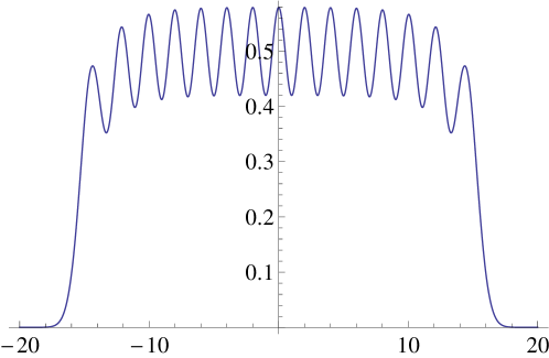
Figure 1: The particle-density profile $\widehat{\rho}_{N}(t,x)$ of the noncolliding Brownian motion with drift at time $t=1$ for $N=15$, where $a=\sigma=1$. The number of nodes is equal to $N=15$. The oscillatory behavior represents the lattice structure in one dimension caused by the present setting of the equidistant initial configuration and well-ordered drift coefficients.

We compare the dependence on time $t$ and particle-number $N$ of density functions between the present process, $\widehat{\rho}_{N}(t,x)$, and the noncolliding Brownian motion without drift started at ${\bf 0}$, denoted by $\widetilde{\rho}_{N}(t,x)$. As reviewed in Sec.5.1 in KT07 , the latter is given by

$$\widetilde{\rho}_{N}(t,x) = \frac{1}{\sqrt{2t}}\sum_{j=0}^{N-1}\left\{\varphi_{j}\left(\frac{x}{\sqrt{2t}}\right)\right\}^{2}$$ (88)

$$= \frac{1}{\sqrt{2t}}\left[N\left\{\varphi_{N}\left(\frac{x}{\sqrt{2t}}\right)\right\}^{2}-\sqrt{N(N+1)}\varphi_{N-1}\left(\frac{x}{\sqrt{2t}}\right)\varphi_{N+1}\left(\frac{x}{\sqrt{2t}}\right)\right],$$

$x\in\mathbb{R},t>0$, where $\varphi_{j}$ is the Hermite function, and it behaves asymptotically in $N\to\infty$ as

$$\widetilde{\rho}_{N}(t,x)\simeq\left\{\begin{array}[]{ll}\displaystyle{\frac{1}{2t\pi}\sqrt{(2\sqrt{Nt})^{2}-x^{2}}},&\quad\mbox{if $|x|\leq 2\sqrt{Nt}$},\\ 0,&\quad\mbox{if $|x|>2\sqrt{Nt}$}.\end{array}\right.$$ (89)

Figure 2 shows (88) at time $t=1$ for $N=1,5,9,13,17$ (from inner to outer). We can observe oscillatory behavior also in this process (the Dyson’s Brownian motion model with $\beta=2$ started at ${\bf 0}$), but the support of density function of $N$ particles can expand only in the order $\sqrt{Nt}$. Therefore, as shown in Fig.2, the ‘wave length of oscillation’ becomes smaller as $\sqrt{t/N}\to 0$ in $N\to\infty$ for each time $0<t<\infty$ and we will have Wigner’s semicircle law (89) for the particle-density profile asymptotically in $N\to\infty$.

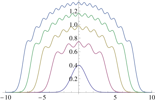
Figure 2: The particle density functions $\widetilde{\rho}_{N}(t,x)$ are plotted at time $t=1$ for $N=1,5,9,13,17$, from inner to outer, for the noncolliding Brownian motion without drift started at ${\bf 0}$. As $N$ becomes large, the profile becomes a semicircle with radius $\propto\sqrt{N}$.

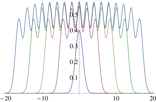
Figure 3: The particle density functions $\widehat{\rho}_{N}(t,x)$ are plotted at time $t=1$ for $N=1,5,9,13,17$, from inner to outer, for the present noncolliding Brownian motion with drift ($a=\sigma=1$). As $N$ becomes large, the support of the profile becomes wider proportionally to $N$. Then the height of the profile is constant and the lattice structure with $N$ nodes is maintained.

On the other hand, Fig.3 shows the particle density functions (87) of the present noncolliding Brownian motion with drift with $t=a=\sigma=1$ for $N=1,5,9,13,17$ (from inner to outer).

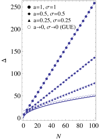
Figure 4: The $N$-dependence of width of density profile $\Delta$ at time $t=1.5$ is shown for $a=\sigma=1$ (dotted by black circles), $a=\sigma=0.5$ (by black squares), $a=\sigma=0.25$ (by black triangles), and for $a=\sigma=0$ (by white circles). For large values of $N$, the dependence is well described by a line $\Delta=c_{1}N+c_{2}$ for the three cases with $a=\sigma>0$; $(c_{1},c_{2})=(2.50,6.29)$ for $a=\sigma=1$, $(c_{1},c_{2})=(1.25,9.70)$ for $a=\sigma=0.5$, $(c_{1},c_{2})=(0.627,15.9)$ for $a=\sigma=0.25$, respectively. The white circles for the noncolliding Brownian motion without drift started at ${\bf 0}$ approaches to the result of Wigner’s semicircle law for the GUE described by a curve $\Delta=4\sqrt{1.5N}\simeq 4.9\sqrt{N}$.

As pointed out by de Haro and Tierz for the case with $\theta=1,q<1$ dHT05 , the width of support of profile increases proportionally to $N$, instead of $\sqrt{N}$. In order to see $N$-dependence numerically, here we define the width $\Delta(t)$ of density profile at a given time $t>0$ as the length of interval of $x$ in which the value of $\widehat{\rho}_{N}$ (or $\widetilde{\rho}_{N}$) is greater than $\varepsilon=0.001$. Figure 4 shows the $N$-dependence of the width at time $t=1.5$, $\Delta=\Delta(1.5)$, for the cases $a=\sigma=1,0.5,0.25$ and for the case $a=\sigma=0$ (the noncolliding Brownian motion without drift started at ${\bf 0}$). By (53), for the first three cases, $\theta=1.5^{-1}\simeq 0.67$ in common and $q\simeq 0.22,0.69$, and 0.91, respectively. In the cases with $a=\sigma>0$ ($q<1$ and $\theta\not=1$ in general), $\Delta$ increases linearly in $N$, while it seems to approach to the curve $\Delta=4\sqrt{1.5N}\simeq 4.9\sqrt{N}$ in the case $a=\sigma=0$ as expected (Wigner’s semicircle law).

Since we put drifts as (13) to particles, $t$-dependence of the support-width is $t$ (drifted), instead of $\sqrt{t}$ (diffusive). In summary, we conjecture that, at each time $0<t<\infty$,

width of support of $$\widehat{\rho}_{N}(t,x)\propto Nt N\to\infty$$ as . (90)

Since $N$ particles exist on the support with width $\propto N$, the average height of density profile becomes independent of $N$ ($\propto 1/t$ in time $t$) and the lattice structure (the oscillatory behavior with $N$ nodes) will not become indistinct even if $N$ is large. Note that by noncolliding condition the particles will show the fermionic (exclusive) behavior. It is in contrast with Wigner’s semicircle law (89), in which the height of profile increases as $N$ becomes large; $\widetilde{\rho}_{N}(t,0)\propto\sqrt{N/t}$.

V Concluding Remarks

In the present paper, we study the noncolliding Brownian motion started at $N$ equidistant points (12) with a period $a$ for which drift coefficients are chosen as (13) with a scale $\sigma$ of values. If we take the double limit $a\to 0$ and $\sigma\to 0$, the process is reduced to the noncolliding Brownian motion without drift started at ${\bf 0}$. It is well-known that, in this limit, the particle-position distribution is equivalent with the eigenvalue distribution of random matrices in GUE with variance $t$ and each time $t>0$ it is a determinantal point process with the correlation kernel expressed by the Hermite polynomials Meh04 ; For10 . We have shown that, for any choice of positive values of parameters $(a,\sigma)$, the determinantal structure of particle distribution is maintained, such that a pair of parameters $(\theta,q)$ are determined at each time $t>0$ by

$$q = q(t)=e^{-\sigma^{2}t},$$ (91)

$$\theta = \theta(t)=\frac{a}{\sigma t},$$ (92)

and the correlation kernel $\mbox{\boldmath$K$}_{N}$ is expressed by the $(\theta,q)$-extensions of the Hermite polynomials, which are the biorthogonal Stieltjes-Wigert polynomials introduced by Dolivet and Tierz DT07 .

As shown by (91), if the system does not have any drift term, $\sigma=0$, then $q\equiv 1$, while if $\sigma>0$, then $q=1$ once at $t=0$ and $q$ decreases monotonically in time $t>0$. Introduction of drifts into the system is essential for the present $q$-extension and the derivation of value $q$ from 1 measures the time $t$. In other words, the present stochastic process is a system with a time-developing $q$-parameter (91). By (92), we see that for each setting of $(a,\sigma)$, there is a unique critical time $t_{0}=a/\sigma$ at which $\theta(t_{0})=1$.

Generalization of Theorem 3 for time correlation functions will be an interesting future problem. The Eynard-Mehta-type correlation kernel EM98 ; BR04 ; KT07 ; KT_cBM shall be discussed.

Invalidity of Wigner’s semicircle law for $q<1$ is an interesting phenomenon, which was first observed by de Haro and Tierz in the case $\theta=1$ dHT05 and is also reported for $\theta\not=1$ in Sec.IV.2 in the present paper. Asymptotic analysis of correlation kernel (86) in $N\to\infty$ will be studied so that the conjecture (90) is proved.

It has been shown here that the present noncolliding Brownian motion with drift is exactly transformed to the biorthogonal Stieltjes-Wigert matrix model studied by Dolivet and Tierz DT07 . We expect further connections in mathematics and physics between nonequilibrium statistical mechanics and the Chern-Simons theory in high-energy physics.

Appendix A Drift Transform and the BBO Formula (5)

First consider a one-dimensional standard Brownian motion without drift started at the origin, $B(t),t\geq 0;B(0)=0$. The probability density at time $t>0$ is given by $u(t,x)=e^{-x^{2}/2t}/\sqrt{2\pi t}$. It solves the diffusion equation $\partial u(t,x)/\partial t=(1/2)\partial^{2}u(t,x)/\partial x^{2}$ and we can see that $u(0,x)\equiv\lim_{t\to 0}u(t,x)=\delta(x)$. Let $\nu\in\mathbb{R}$ and consider the diffusion equation with a drift term

$$\frac{\partial}{\partial t}u^{\nu}(t,x)=\frac{1}{2}\frac{\partial^{2}}{\partial x^{2}}u^{\nu}(t,x)+\nu\frac{\partial}{\partial x}u^{\nu}(t,x).$$ (93)

A solution is given by

$$u^{\nu}(t,x) = u(t,x+\nu t)$$ (94)

$$= \frac{1}{\sqrt{2\pi t}}\exp\left\{-\frac{1}{2t}(x+\nu t)^{2}\right\}.$$

The mean of the Gaussian distribution is shifted by $-\nu t$, that is, $-\nu$ gives a drift velocity. We note that (94) is written as $u^{\nu}(t,x)=e^{-\nu x-\nu^{2}t/2}u(t,x)$. It is considered as follows (see, for instance, KS91 ); $u^{\nu}(t,x)$ is obtained from $u(t,x)$ by the drift transform,

$$u(t,x)\,\to\,\exp\left(-\nu x-\frac{\nu^{2}}{2}t\right)u(t,x).$$ (95)

The transition probability density from $x$ to $y$ with time duration $t$ is then obtained by a shift of spatial coordinate

$$p^{\nu}(t,y|x) = u^{\nu}(t,x-y)$$ (96)

$$= \exp\left\{\nu(y-x)-\frac{\nu^{2}}{2}t\right\}p(t,y|x),$$

where $p(t,y|x)$ is given by (7). Note that (96) satisfies the diffusion equation (93) as a backward Kolmogorov equation.

Let $N=2,3,\dots$. Consider the vicious Brownian motion defined as

$$N$$-particle system of Brownian motion killed when they collide

$$= N \mathbb{W}_{N}$$ -dimensional Brownian motion in the Weyl chamber with absorbing walls.

The transition probability density from $\mbox{\boldmath$x$}\in\mathbb{W}_{N}$ to $\mbox{\boldmath$y$}\in\mathbb{W}_{N}$ with time duration $t\geq 0$ is given by the KM-LGV determinant $q_{N}(t,\mbox{\boldmath$y$}|\mbox{\boldmath$x$})$, (6). It is a unique solution of the differential equation

$$\frac{\partial}{\partial t}u(t,\mbox{\boldmath$x$})=\frac{1}{2}\Delta u(t,\mbox{\boldmath$x$}),\quad\Delta\equiv\sum_{j=1}^{N}\frac{\partial^{2}}{\partial x_{j}^{2}},$$ (97)

satisfying the boundary condition $u(t,\mbox{\boldmath$x$})=0$ at $\mbox{\boldmath$x$}\in\partial\mathbb{W}_{N}$, and the initial condition $u(0,\mbox{\boldmath$x$})=\delta(\mbox{\boldmath$x$}-\mbox{\boldmath$y$})=\prod_{j=1}^{N}\delta(x_{j}-y_{j})$.

Now we consider the vicious Brownian motion problem with drift. For $\mbox{\boldmath$\nu$}=(\nu_{1},\dots,\nu_{N})\in\mathbb{R}^{N}$, we want to solve

$$\frac{\partial}{\partial t}u(t,\mbox{\boldmath$x$})=\frac{1}{2}\Delta u(t,\mbox{\boldmath$x$})+\mbox{\boldmath$\nu$}\cdot\nabla u(t,\mbox{\boldmath$x$})$$ (98)

with the conditions

$$u(t,\mbox{\boldmath$x$})>0,\quad\mbox{\boldmath$x$}\in\mathbb{W}_{N},t>0,$$

$$u(t,\mbox{\boldmath$x$})=0\quad\mbox{at $\mbox{\boldmath$x$}\in\partial\mathbb{W}_{N},t>0$},$$

$$u(0,\mbox{\boldmath$x$})=\delta(\mbox{\boldmath$x$}-\mbox{\boldmath$y$}).$$ (99)

The solution is given by the drift transform of the KM-LGV determinant (6),

$$q_{N}^{\mbox{\boldmath$\nu$}}(t,\mbox{\boldmath$y$}|\mbox{\boldmath$x$}) = \exp\left\{\mbox{\boldmath$\nu$}\cdot(\mbox{\boldmath$y$}-\mbox{\boldmath$x$})-\frac{|\mbox{\boldmath$\nu$}|^{2}}{2}t\right\}q_{N}(t,\mbox{\boldmath$y$}|\mbox{\boldmath$x$})$$ (100)

$$= \exp\left\{\mbox{\boldmath$\nu$}\cdot(\mbox{\boldmath$y$}-\mbox{\boldmath$x$})-\frac{|\mbox{\boldmath$\nu$}|^{2}}{2}t\right\}\det_{1\leq j,k\leq N}\Big{[}p(t,y_{j}|x_{k})\Big{]}.$$

The important fact is that

$$q_{N}^{\mbox{\boldmath$\nu$}}(t,\mbox{\boldmath$y$}|\mbox{\boldmath$x$})\not=\det_{1\leq j,k\leq N}\Big{[}p^{\nu_{j}}(t,y_{j}|\mbox{\boldmath$x$}_{k})\Big{]}.$$

That is, it is not the KM-LGV determinant of the drift transform of $p$’s. Actually we can see

$$q_{N}^{\mbox{\boldmath$\nu$}}(t,\mbox{\boldmath$y$}|\mbox{\boldmath$x$}) = e^{-\mbox{\boldmath$\nu$}\cdot\mbox{\boldmath$x$}}\sum_{\sigma\in{\cal S}_{N}}{\rm sgn}(\sigma)\prod_{k=1}^{N}e^{\nu_{k}x_{\sigma(k)}}\prod_{j=1}^{N}p(t,y_{j}-\nu_{j}t|x_{\sigma(j)})$$ (101)

$$= e^{-\mbox{\boldmath$\nu$}\cdot\mbox{\boldmath$x$}}\sum_{\sigma\in{\cal S}_{N}}{\rm sgn}(\sigma)\prod_{k=1}^{N}e^{\nu_{k}x_{\sigma(k)}}\prod_{j=1}^{N}p^{\nu_{j}}(t,y_{j}|x_{\sigma(j)}),$$

where ${\cal S}_{N}$ is the set of all permutations $\{\sigma\}$ of $N$ items.

The survival probability at time $t>0$ will be given by

$${\cal N}_{N}^{\mbox{\boldmath$\nu$}}(t,\mbox{\boldmath$x$}) = \int_{\mathbb{W}_{N}}q_{N}^{\mbox{\boldmath$\nu$}}(t,\mbox{\boldmath$y$}|\mbox{\boldmath$x$})d\mbox{\boldmath$y$}$$ (102)

$$= e^{-\mbox{\boldmath$\nu$}\cdot\mbox{\boldmath$x$}}\sum_{\sigma\in{\cal S}_{N}}{\rm sgn}(\sigma)\prod_{k=1}^{N}e^{\nu_{k}x_{\sigma(k)}}\int_{\mathbb{W}_{N}}\prod_{j=1}^{N}p^{\nu_{j}}(t,y_{j}|x_{\sigma(j)})d\mbox{\boldmath$y$}.$$

It was claimed in BBO05 that

if $$\mbox{\boldmath$\nu$}\in\mathbb{W}_{N} \mbox{\boldmath$x$}\in\mathbb{W}_{N}$$ and (103)

then

$$\lim_{t\to\infty}\int_{\mathbb{W}_{N}}\prod_{j=1}^{N}p^{\nu_{j}}(t,y_{j}|x_{\sigma(j)})d\mbox{\boldmath$y$}=1,\quad\forall\sigma\in{\cal S}_{N}.$$ (104)

That is, for any initial configuration $\mbox{\boldmath$x$}\in\mathbb{R}^{N}$, if (103) is satisfied,

$$\lim_{t\to\infty}\mbox{\boldmath$B$}^{\mbox{\boldmath$x$},\mbox{\boldmath$\nu$}}(t)\in\mathbb{W}_{N}\quad\mbox{with probab. 1.}$$ (105)

It is a matter of course, since we put the drift vector $\mbox{\boldmath$\nu$}\in\mathbb{W}_{N}$, the position vector of Brownian motions should be in $\mathbb{W}_{N}$ if we wait for sufficiently long term, independently of initial configuration. Then we obtain BBO05

$$\lim_{t\to\infty}{\cal N}_{N}^{\mbox{\boldmath$\nu$}}(t,\mbox{\boldmath$x$}) = e^{-\mbox{\boldmath$\nu$}\cdot\mbox{\boldmath$x$}}\sum_{\sigma\in{\cal S}_{N}}{\rm sgn}(\sigma)\prod_{k=1}^{N}e^{\nu_{k}x_{\sigma(k)}}$$ (106)

$$= e^{-\mbox{\boldmath$\nu$}\cdot\mbox{\boldmath$x$}}\det_{1\leq j,k\leq N}\Big{[}e^{\nu_{j}x_{k}}\Big{]}.$$

Remark 5   The following argument is found in OCo12b . Let $S_{N}^{\mbox{\boldmath$\nu$}}(\mbox{\boldmath$x$})$ be the survival probability for the noncolliding BM with drift $\mbox{\boldmath$\nu$}\in\mathbb{W}_{N}$ started at $\mbox{\boldmath$x$}\in\mathbb{W}_{N}$. Then, it is a stationary solution of the diffusion equation

$$0=\frac{1}{2}\Delta S_{N}^{\mbox{\boldmath$\nu$}}(\mbox{\boldmath$x$})+\mbox{\boldmath$\nu$}\cdot\nabla S_{N}^{\mbox{\boldmath$\nu$}}(\mbox{\boldmath$x$}),$$ (107)

satisfying the conditions

$$S_{N}^{\mbox{\boldmath$\nu$}}(\mbox{\boldmath$x$})=0\quad\mbox{at $\mbox{\boldmath$x$}\in\partial\mathbb{W}_{N}$},$$

$$\lim_{\mbox{\boldmath$x$}\to\infty}S_{N}^{\mbox{\boldmath$\nu$}}(\mbox{\boldmath$x$})=1,$$ (108)

where

$$\mbox{\boldmath$x$}\to\infty\quad\Longleftrightarrow\quad x_{j+1}-x_{j}\to\infty,\quad 1\leq j\leq N-1.$$

We can confirm that

$$e^{-\mbox{\boldmath$\nu$}\cdot\mbox{\boldmath$x$}}\det_{1\leq j,k\leq N}\Big{[}e^{\nu_{j}x_{k}}\Big{]}$$

is the unique solution of this problem.

The noncolliding Brownian motion with drift is defined as the system of Brownian motions conditioned that they never collide with each other forever. Then, the transition probability density is obtained by

$$p_{N}^{\mbox{\boldmath$\nu$}}(t,\mbox{\boldmath$y$}|\mbox{\boldmath$x$}) = \lim_{T\to\infty}\frac{{\cal N}^{\mbox{\boldmath$\nu$}}(T-t,\mbox{\boldmath$y$})q_{N}^{\mbox{\boldmath$\nu$}}(t,\mbox{\boldmath$y$}|\mbox{\boldmath$x$})}{{\cal N}^{\mbox{\boldmath$\nu$}}(T,\mbox{\boldmath$x$})}$$

$$= \frac{e^{-\mbox{\boldmath$\nu$}\cdot\mbox{\boldmath$y$}}\displaystyle{\det_{1\leq j,k\leq N}[e^{\nu_{j}y_{k}}]}}{e^{-\mbox{\boldmath$\nu$}\cdot\mbox{\boldmath$x$}}\displaystyle{\det_{1\leq j,k\leq N}[e^{\nu_{j}x_{k}}]}}e^{\mbox{\boldmath$\nu$}\cdot(\mbox{\boldmath$y$}-\mbox{\boldmath$x$})-|\mbox{\boldmath$\nu$}|^{2}t/2}q_{N}(t,\mbox{\boldmath$y$}|\mbox{\boldmath$x$}).$$

It is equal to (5).

Appendix B A Combinatorial Limit of O’Connell Process

Recently O’Connell introduced an interacting diffusive particle system OCo12a . Let $\psi_{\mbox{\boldmath$\nu$}}^{(N)}(\mbox{\boldmath$x$}),\mbox{\boldmath$x$}\in\mathbb{R}^{N},\mbox{\boldmath$\nu$}\in\mathbb{C}^{N}$ (the $N$-dimensional complex space) be the class-one Whittaker function, whose Givental integral representation is given by

$$\psi_{\mbox{\boldmath$\nu$}}^{(N)}(\mbox{\boldmath$x$}) = \int_{\Gamma_{N}(\mbox{\boldmath$x$})}\exp\left[\sum_{j=1}^{N}\nu_{j}\left(\sum_{k=1}^{j}T_{j,k}-\sum_{k=1}^{j-1}T_{j-1,k}\right)\right.$$ (109)

$$\quad\left.-\sum_{j=1}^{N-1}\sum_{k=1}^{j}\Big{\{}e^{-(T_{j,k}-T_{j+1,k})}+e^{-(T_{j+1,k+1}-T_{j,k})}\Big{\}}\right]d\mbox{\boldmath$T$},$$

where the integral is performed over the space of all real lower triangular arrays with size $N$, $\mbox{\boldmath$T$}=(T_{j,k},1\leq k\leq j\leq N)$ conditioned $T_{N,k}=x_{k},1\leq k\leq N$. The transition probability density $P_{N}^{\mbox{\boldmath$\nu$},\,a}$ of the O’Connell process with a parameter $a>0$ Kat12a is a unique solution of the equation

$$\left[\frac{\partial}{\partial t}-\left(\frac{1}{2}\Delta+\nabla\log\psi^{(N)}_{\mbox{\boldmath$\nu$}}(\mbox{\boldmath$x$}/a)\cdot\nabla\right)\right]P_{N}^{\mbox{\boldmath$\nu$},\,a}(t,\mbox{\boldmath$y$}|\mbox{\boldmath$x$})=0$$ (110)

with the initial condition $P_{N}^{\mbox{\boldmath$\nu$},\,a}(0,\mbox{\boldmath$y$}|\mbox{\boldmath$x$})=\delta(\mbox{\boldmath$x$}-\mbox{\boldmath$y$})$. The solution is given by

$$P_{N}^{\mbox{\boldmath$\nu$},\,a}(t,\mbox{\boldmath$y$}|\mbox{\boldmath$x$})=e^{-t|\mbox{\boldmath$\nu$}|^{2}/2a^{2}}\frac{\psi^{(N)}_{\mbox{\boldmath$\nu$}}(\mbox{\boldmath$y$}/a)}{\psi^{(N)}_{\mbox{\boldmath$\nu$}}(\mbox{\boldmath$x$}/a)}Q_{N}^{a}(t,\mbox{\boldmath$y$}|\mbox{\boldmath$x$})$$ (111)

with

$$Q_{N}^{a}(t,\mbox{\boldmath$y$}|\mbox{\boldmath$x$})=\int_{\mathbb{R}^{N}}e^{-t|\mbox{\boldmath$k$}|^{2}/2}\psi^{(N)}_{ia\mbox{\boldmath$k$}}(\mbox{\boldmath$x$}/a)\psi^{(N)}_{-ia\mbox{\boldmath$k$}}(\mbox{\boldmath$y$}/a)s_{N}(a\mbox{\boldmath$k$})d\mbox{\boldmath$k$},$$ (112)

where $i=\sqrt{-1}$ and $s_{N}(\mbox{\boldmath$\mu$})$ is the density function of the Sklyanin measure

$$s_{N}(\mbox{\boldmath$\mu$})=\frac{1}{(2\pi)^{N}!}\prod_{1\leq j<\ell\leq N}|\Gamma(i(\mu_{\ell}-\mu_{j}))|^{-2}.$$ (113)

We can show that (110) is a geometric lifting with parameter $a>0$ of the diffusion equation (the backward Kolmogorov equation) of the noncolliding Brownian motion with drift Kat11 ; Kat12a . Then the BBO formula (5) is regarded as a combinatorial limit of the transition probability density of the O’Connell process in the sense that Kat12b ; Kat12c

$$p_{N}^{\mbox{\boldmath$\nu$}}(t,\mbox{\boldmath$y$}|\mbox{\boldmath$x$})=\lim_{a\to 0}P_{N}^{a\mbox{\boldmath$\nu$},\,a}(t,\mbox{\boldmath$y$}|\mbox{\boldmath$x$}),\quad\mbox{\boldmath$x$},\mbox{\boldmath$\nu$}\in\overline{\mathbb{W}}_{N},\,\mbox{\boldmath$y$}\in\mathbb{W}_{N},\,t\in[0,\infty).$$ (114)

We note that the above argument (the geometric lifting and combinatorial limit) gives another proof of the BBO formula (5) for the noncolliding Brownian motion with drift.

Appendix C Geometric Brownian Motion

For $\sigma\not=0,\mu\in\mathbb{R}$, and $x>0$ consider the linear stochastic differential equation (SDE)

$$dX(t)=\sigma X(t)dB(t)+\mu X(t)dt,\quad X(0)=x,\quad t\geq 0,$$ (115)

where $B(t),t\geq 0$ is a standard Brownian motion started at 0. The parameters $\sigma$ and $\mu$ are called percentage volatility and percentage drift, respectively. The process $X(t),t\geq 0$ is called a geometric (or exponential) Brownian motion BS02 . The backward Kolmogorov equation for the process $X(t)$ is given by

$$\frac{\partial}{\partial t}u(t,x)=\frac{1}{2}\sigma^{2}x^{2}\frac{\partial^{2}}{\partial x^{2}}u(t,x)+\mu x\frac{\partial}{\partial x}u(t,x).$$ (116)

Set

$$\widetilde{\nu}=\frac{1}{\sigma^{2}}\left(\mu-\frac{\sigma^{2}}{2}\right)\quad\Longleftrightarrow\quad\mu=\frac{2\widetilde{\nu}+1}{2}\sigma^{2},$$ (117)

and put

$$p(t;x,y)=\frac{|\sigma|}{2\sqrt{2\pi t}}(xy)^{-\widetilde{\nu}}\exp\left(-\frac{\sigma^{2}\widetilde{\nu}^{2}t}{2}-\frac{(\ln y-\ln x)^{2}}{2\sigma^{2}t}\right).$$ (118)

It is easy to confirm that (118) satisfies the backward Kolmogorov equation (116). Remark that $p(t;x,y)$ is symmetric with respect to $x$ and $y$; $p(t;x,y)=p(t;y,x)$.

Let

$$m(dx)=\frac{2}{\sigma^{2}}x^{2\widetilde{\nu}-1}dx,$$ (119)

which is called the speed measure of $X(t)$. By the general theory of one-dimensional diffusion processes BS02 , it is proved that for any $A\subset\mathbb{R}$ the probability $P_{t}(x,A)={\rm Prob}(X(t)\in A|X(0)=x)$ is given by $P_{t}(x,A)=\int_{A}p(t;x,y)m(dy).$ In other words, if we set

$$p(t,y|x)=p(t;x,y)\frac{m(dy)}{dy},$$ (120)

then $p(t,y|x)$ is the transition probability density of the process from $x\in\mathbb{R}_{+}$ to $y\in\mathbb{R}_{+}$ during time $t>0$; $P_{t}(x,A)=\int_{A}p(t,y|x)dy.$ From (118) and (119), we have the following expressions,

$$p(t,y|x) = \frac{2}{\sigma^{2}}y^{2\widetilde{\nu}-1}\frac{|\sigma|}{2\sqrt{2\pi t}}(xy)^{-\widetilde{\nu}}\exp\left(-\frac{\sigma^{2}\widetilde{\nu}^{2}t}{2}-\frac{(\ln y-\ln x)^{2}}{2\sigma^{2}t}\right)$$ (121)

$$= \frac{1}{y|\sigma|\sqrt{2\pi t}}\left(\frac{y}{x}\right)^{\widetilde{\nu}}\exp\left(-\frac{\sigma^{2}\widetilde{\nu}^{2}t}{2}-\frac{(\ln y-\ln x)^{2}}{2\sigma^{2}t}\right)$$

$$= \frac{1}{y|\sigma|\sqrt{2\pi t}}\exp\left\{-\frac{1}{2\sigma^{2}t}\Big{(}\ln(y/x)-\widetilde{\nu}\sigma^{2}t\Big{)}^{2}\right\}.$$

Let

$$\sigma_{t} = |\sigma|\sqrt{t},$$

$$\mu_{t}(x) = \ln x+\widetilde{\nu}\sigma^{2}t=\ln x+\widetilde{\nu}\sigma_{t}^{2}.$$ (122)

Then (121) is written as

$$p(t,y|x)=\frac{1}{y\sigma_{t}\sqrt{2\pi}}\exp\left\{-\frac{(\ln y-\mu_{t}(x))^{2}}{2\sigma_{t}^{2}}\right\}.$$ (123)

It is nothing but the log-normal distribution with parameters $\sigma_{t}$ and $\mu_{t}(x)$.

In the present paper we consider the case

$$\widetilde{\nu}=0\quad\Longleftrightarrow\quad\mu=\frac{\sigma^{2}}{2}.$$ (124)

That is, the SDE is given by

$$dX(t)=\sigma X(t)dB(t)+\frac{\sigma^{2}}{2}X(t)dt,\quad t\geq 0,$$ (125)

By a simple application of Itô’s formula KS91 , we can confirm that the solution of this SDE is given by (25).

Appendix D Noncolliding Geometric Brownian Motion

For arbitrary $M\in\mathbb{N},0<t_{1}<\cdots<t_{M}<\infty$, the multitime joint probability density for the noncolliding Brownian motion without drift is given by KT07 ; KT10

$$p_{N}(t_{1},\mbox{\boldmath$x$}^{(1)};\dots;t_{M},\mbox{\boldmath$x$}^{(M)}|\mbox{\boldmath$x$})$$

$$=\prod_{1\leq j<k\leq N}(x^{(M)}_{k}-x^{(M)}_{j})\prod_{m=1}^{M-1}q_{N}(t_{m+1}-t_{m},\mbox{\boldmath$x$}^{(m+1)}|\mbox{\boldmath$x$}^{(m)})\frac{q_{N}(t_{1},\mbox{\boldmath$x$}^{(1)}|\mbox{\boldmath$x$})}{\prod_{1\leq j<k\leq N}(x_{k}-x_{j})}$$ (126)

for any fixed initial configuration $\mbox{\boldmath$x$}=(x_{1},\dots,x_{N})\in\overline{\mathbb{W}}_{N}$.

By the transformation (25) from $B(t)\to X(t),t\geq 0$, the $N$-particle system of geometric Brownian motions with percentage volatility $\sigma>0$ conditioned never to collide with each other, which we call the noncolliding geometric Brownian motion, should have the multitime joint probability density in the form

$$p_{N}(t_{1},\mbox{\boldmath$y$}^{(1)};\dots;t_{M},\mbox{\boldmath$y$}^{(M)}|\mbox{\boldmath$y$})=\prod_{1\leq j<k\leq N}(\ln y^{(M)}_{k}-\ln y^{(M)}_{j})$$

$$\qquad\qquad\times\prod_{m=1}^{M-1}q_{N}^{\rm geo}(t_{m+1}-t_{m},\mbox{\boldmath$y$}^{(m+1)}|\mbox{\boldmath$y$}^{(m)})\frac{q_{N}^{\rm geo}(t_{1},\mbox{\boldmath$y$}^{(1)}|\mbox{\boldmath$y$})}{\prod_{1\leq j<k\leq N}(\ln y_{k}-\ln y_{j})}.$$ (127)

It does not seem to be possible to derive (21) from this general formula by just choosing an initial configuration $y$.

References

- (1) M. E. Fisher, Walks, walls, wetting, and melting, J. Stat. Phys. 34, 667-729 (1984).
- (2) F. J. Dyson, A Brownian-motion model for the eigenvalues of a random matrix, J. Math. Phys. 3, 1191-1198 (1962).
- (3) M. Katori and H. Tanemura, Noncolliding Brownian motion and determinantal processes, J. Stat. Phys. 129, 1233-1277 (2007).
- (4) M. Katori and H. Tanemura, Noncolliding processes, matrix-valued processes and determinantal processes, Sugaku Expositions 24, 263-289 (2011); e-print arXiv:1005.0533 [math.PR.].
- (5) T. Nagao and P. J. Forrester, Multilevel dynamical correlation function for Dyson’s Brownian motion model of random matrices, Phys. Lett. A247, 42-46 (1998).
- (6) P. J. Forrester, T. Nagao, and G. Honner, Correlations for the orthogonal-unitary and symplectic-unitary transitions at the hard and soft edges, Nucl. Phys. B 553[PM], 601-643 (1999).
- (7) D. J. Grabiner, Brownian motion in a Weyl chamber, non-colliding particles, and random matrices, Ann. Inst. Henri Poincaré, Probab. Stat. 35, 177-204 (1999).
- (8) J. Baik, Random vicious walks and random matrices, Commun. Pure Appl. Math. 53, 1385-1410 (2000).
- (9) K. Johansson, Non-intersecting paths, random tilings and random matrices, Probab. Th. Rel. Fields 123, 225-280 (2002).
- (10) T. Nagao and P. J. Forrester, Vicious random walkers and a discretization of Gaussian random matrix ensembles, Nucl. Phys. B 620[FS], 551-565 (2002).
- (11) M. Katori and H. Tanemura, Scaling limit of vicious walks and two-matrix model, Phys. Rev. E 66, 011105 (2002).
- (12) T. Nagao, M. Katori, and H. Tanemura, Dynamical correlations among vicious random walkers, Phys. Lett. A 307, 29-35 (2003).
- (13) M. Katori and H. Tanemura, Symmetry of matrix-valued stochastic processes and noncolliding diffusion particle systems, J. Math. Phys. 45, 3058-3085 (2004).
- (14) M. Katori and H. Tanemura, Non-equilibrium dynamics of Dyson’s model with an infinite number of particles, Commun. Math. Phys. 293, 469-497 (2010).
- (15) C. A. Tracy and H. Widom, Level-spacing distributions and the Airy kernel, Commun. Math. Phys. 159, 151-174 (1994).
- (16) C. A. Tracy and H. Widom, On the orthogonal and symplectic matrix ensembles, Commun. Math. Phys. 177, 727-754 (1996).
- (17) C. A. Tracy and H. Widom, Differential equations for Dyson processes, Commun. Math. Phys. 252, 7-41 (2004).
- (18) C. A. Tracy and H. Widom, Nonintersecting Brownian excursions, Ann. Appl. Probab. 17, 953-979 (2007).
- (19) M. Katori, M. Izumi, and N. Kobayashi, Two Bessel bridges conditioned never to collide, double Dirichlet series, and Jacobi theta function, J. Stat. Phys. 131, 1067-1083 (2008).
- (20) G. Schehr, S. N. Majumdar, A. Comtet, and J. Randon-Furling, Exact distribution of the maximal height of vicious walkers, Phys. Rev. Lett. 101, 150601 (2008).
- (21) N. Kobayashi, M. Izumi, and M. Katori, Maximum distributions of bridges of noncolliding Brownian paths, Phys. Rev. E 78, 051102 (2008).
- (22) P. J. Forrester, S. N. Majumdar, and G. Schehr, Non-intersecting Brownian walkers and Yang-Mills theory on the sphere, Nucl. Phys. B 844, 500-526 (2011).
- (23) K. Liechty, Nonintersecting Brownian motions on the half-line and discrete Gaussian orthogonal polynomials, J. Stat. Phys. 147, 582-622 (2012).
- (24) A. J. Guttmann, A. L. Owczarek, and X. G. Viennot, Vicious walkers and Young tableaux I: Without walls, J. Phys. A 31, 8123-8135 (1998).
- (25) C. Krattenthaler, A. J. Guttmann, and X. G. Viennot, Vicious walkers, friendly walkers and Young tableaux II: With a wall, J. Phys. A 33, 8835-8866 (2000).
- (26) D. K. Arrowsmith, F. M. Bhatti, and J. W. Essam, Maximum Fermi walk configurations on the directed square lattice and standard Young tableaux, J. Phys. A 43, 145206 (2010).
- (27) T. Feierl, The height of watermelons with wall, J. Phys. A 45, 095003 (2012).
- (28) D. K. Arrowsmith, F. M. Bhatti, and J. W. Essam, Bose and Fermi walk configurations on planar graphs, J. Phys. A 45, 225003 (2012).
- (29) A. B. J. Kuijlaars, A. Martinez-Finkelstein, and F. Wielonsky, Non-intersecting squared Bessel paths and multiple orthogonal polynomials for modified Bessel weights, Commun. Math. Phys. 286, 217-275 (2009).
- (30) S. Delvaux, A. B. J. Kuijlaars, L. Zhang, Critical behavior of nonintersecting Brownian motions at a tacnode, Commun. Pure Appl. Math. 64, 1305-1383 (2011).
- (31) A. B. J. Kuijlaars, A. Martinez-Finkelstein, and F. Wielonsky, Non-intersecting squared Bessel paths: Critical time and double scaling limit, Commun. Math. Phys. 308, 227-279 (2011).
- (32) J. Cardy and M. Katori, Families of vicious walkers, J. Phys. A 36, 609-629 (2003).
- (33) I. Goncharenko and A. Gopinathan, Vicious walks with long-range interactions, Phys. Rev. E 82, 011126 (2010).
- (34) I. Goncharenko and A. Gopinathan, Vicious Levy flights, Phys. Rev. Lett. 105, 190601 (2010).
- (35) M. Prähofer and H. Spohn, Scale invariance of the PNG droplet and the Airy process, J. Stat. Phys. 108, 1071-1106 (2002).
- (36) K. Johansson, Discrete polynuclear growth and determinantal processes, Commun. Math. Phys. 242, 277-329 (2003).
- (37) T. Imamura and T. Sasamoto, Polynuclear growth model with external source and random matrix model with deterministic source, Phys. Rev. E 71, 041606 (2005).
- (38) M. Katori, O’Connell’s process as a vicious Brownian motion, Phys. Rev. E 84, 061144 (2011).
- (39) N. O’Connell, Directed polymers and the quantum Toda lattice, Ann. Probab. 40, 437-458 (2012).
- (40) M. Katori, Survival probability of mutually killing Brownian motion and the O’Connell process, J. Stat. Phys. 147, 206-223 (2012).
- (41) S. Karlin and J. McGregor, Coincidence probabilities, Pacific J. Math. 9, 1141-1164 (1959).
- (42) B. Lindström, On the vector representations of induced matroids, Bull. London Math. Soc. 5, 85-90 (1973).
- (43) I. Gessel and G. Viennot, Binomial determinants, paths, and hook length formulae, Adv. Math. 58, 300-321 (1985).
- (44) P. Biane, P.Bougerol, and N. O’Connell, Littelmann paths and Brownian paths, Duke Math. J. 130, 127-167 (2005).
- (45) W. Fulton and J. Harris, Representation Theory, A First Course, (Springer, New York, 1991).
- (46) M. L. Mehta, Random Matrices, 3rd edn., (Elsevier, Amsterdam, 2004).
- (47) P. J. Forrester, Log-gases and Random Matrices, London Mathematical Society Monographs, (Princeton University Press, Princeton, 2010).
- (48) M. Katori, Determinantal process starting from an orthogonal symmetry is a Pfaffian process, J. Stat. Phys. 146, 249-263 (2012).
- (49) P. Biane, P. Bougerol, and N. O’Connell, Continuous crystal and Duistermaat-Heckman measure for Coxeter groups, Adv. Math. 221, 1522-1583 (2009).
- (50) N. O’Connell, Whittaker functions and related stochastic processes, e-print arXiv:1201.4849 [math.PR.].
- (51) M. Katori, Reciprocal time relation of noncolliding Brownian motion with drift, J. Stat. Phys. 148, 38-52 (2012).
- (52) M. Katori, System of complex Brownian motions associated with the O’Connell process, J. Stat. Phys. (in press); e-print arXiv:1206.2185 [math.PR.].
- (53) A. Borodin and I. Corwin, Macdonald processes, e-print arXiv:1111.4408 [math.PR.].
- (54) Y. Dolivet and M. Tierz, Chern-Simons matrix models and Stieltjes-Wigert polynomials, J. Math. Phys. 48, 023507 (2007).
- (55) K. A. Muttalib, Random matrix models with additional interactions, J. Phys. A 285, L159-L164 (1995).
- (56) A. Borodin, Biorthogonal ensembles, Nucl. Phys. B 536, 704-732 (1999).
- (57) G. Szegö, Orthogonal Polynomials, 4th edn., (American Mathematical Society, 1981).
- (58) R. Koekoek and R. Swarttouw, The Askey-scheme of hypergeometric orthogonal polynomials and its -analogue, e-print arXiv:9602214 [math.CA.].
- (59) A. Soshnikov, Determinantal random point fields, Russian Math. Surveys 55, 923-975 (2000).
- (60) T. Shirai and Y. Takahashi, Random point fields associated with certain Fredholm determinants I: Fermion, Poisson and boson point process, J. Funct. Anal. 205, 414-463 (2003).
- (61) A. N. Borodin and P. Salminen, Handbook of Brownian Motion – Facts and Formulae, 2nd edn., (Birkhäuser, 2002).
- (62) M. Tierz, Schur polynomials and biorthogonal random matrix ensemble, J. Math. Phys. 51, 063509 (2010).
- (63) M. Tierz, Soft matrix models and Chern-Simons partition functions, Mod. Phys. Lett. A19, 1365-1378 (2004).
- (64) M. Mariño, Chern-Simons theory, matrix integrals, and perturbative three-manifold invariants, Commun. Math. Phys. 253, 25-49 (2005).
- (65) S. de Haro and M. Tierz, Discrete and oscillatory matrix models in Chern-Simons theory, Nucl. Phys. B 731 [FS], 225-241 (2005).
- (66) W. A. Al-Salam and A. Verma, -Konhauser polynomials, Pac. J. Math. 108, 1-7 (1983).
- (67) B. Eynard, M. L. Mehta, Matrices coupled in a chain I: Eigenvalue correlations, J. Phys. A 31, 4449-4456 (1998).
- (68) A. Borodin and E. M. Rains, Eynard-Mehta theorem, Schur process, and their pfaffian analogs, J. Stat. Phys. 121, 291-317 (2005).
- (69) M. Katori and H. Tanemura, Complex Brownian motion representation of the Dyson model, e-print arXiv:1008.2821 [math.PR.].
- (70) I. Karatzas, S. E. Shreve, Brownian Motion and Stochastic Calculus, 2nd ed., (Springer, New York, 1991).