Resummation Effects in Vector-Boson and Higgs Associated Production
Abstract
Fixed-order QCD radiative corrections to the vector-boson and Higgs associated production channels, (), at hadron colliders are well understood. We combine higher order perturbative QCD calculations with soft-gluon resummation of both threshold logarithms and logarithms which are important at low transverse momentum of the pair. We study the effects of both types of logarithms on the scale dependence of the total cross section and on various kinematic distributions. The next-to-next-to-next-to-leading logarithmic (NNNLL) resummed total cross sections at the LHC are almost identical to the fixed-order perturbative next-to-next-to-leading order (NNLO) rates, indicating the excellent convergence of the perturbative QCD series. Resummation of the transverse momentum () spectrum provides reliable results for small values of and suggests that implementing a jet-veto will significantly decrease the cross sections.
I Introduction
The recent discovery of a Higgs-like particle Gianotti (July 4, 2012); Incandela (July 4, 2012) has brought our understanding of electroweak symmetry breaking to a deeper level. Now it is imperative to study the detailed properties of this particle in the hope of finding any hints for new physics beyond the Standard Model (SM). An important Higgs production mechanism at hadron colliders is the associated production of a Higgs boson and a vector boson, Glashow et al. (1978). At the Tevatron, the process with the decay of the vector boson to leptons and of the Higgs to the and channels has provided important sensitivity to a light Higgs boson Stange et al. (1994); CDF and Collaborations (2012). At the LHC, the production rate for associated production is small, but with a light Higgs in association with a or can potentially be observed in the boosted regime via Butterworth et al. (2008). Reliable predictions are essential for the observation and study of the couplings in this channel Dittmaier et al. (2011, 2012).
The rate for associated production is perturbatively known to next-to-next-to-leading order (NNLO), i.e. Brein et al. (2004, 2012). At next-to-leading order (NLO), the QCD corrections are identical to those of the Drell-Yan process for an off-shell gauge boson, Han and Willenbrock (1991); Baer et al. (1993); Ohnemus and Stirling (1993). At NNLO, however, the process receives a small additional contribution from the initial state, Brein et al. (2004). The NLO rates are available in the general purpose MCFM J.Campbell et al. (2012) program, while the total rate can be found to NNLO using the VH@NNLO code Brein et al. (2004).
Infrared finite results in higher-order QCD processes occur due to a cancellation of virtual and real soft divergences. The fixed-order calculation is reliable providing all of the scales are of the same order of magnitude. When the invariant mass of the final state particles or approaches the center-of-mass energy of the colliding partons, there is less phase space available for real emission. While the infrared divergences will still cancel, large Sudakov logarithms will remain. These logarithms can spoil the convergence of the perturbative series and need to be resummed to all orders for reliable results in this threshold region Collins et al. (1985). Threshold corrections involve terms of the form , which are large when , where is the partonic center-of-mass (c.m.) energy-squared Sterman (1987); Catani et al. (1996); Catani and Trentadue (1989); Sterman and Vogelsang (2001); Becher et al. (2008). Similarly, large logarithms of the form can also occur when the system is produced with small transverse momentum Bozzi et al. (2006); Catani et al. (2001). The techniques for resumming both types of logarithms to all orders are well known and the fixed order perturbative and resummed calculations can be consistently matched at intermediate values of the kinematic variables.
We consider the process and present results from both the threshold resummation and the transverse momentum resummation of large logarithms separately for LHC energies. Since the final state particles are color-singlets, both types of resummation can be straight-forwardly adopted from results in the literature for the Drell-Yan process Becher et al. (2008); Catani et al. (2001); Bozzi et al. (2006); Arnold and Kauffman (1991); Han et al. (1992). (We do not discuss the joint resummation of the logarithms Kulesza et al. (2002)). Section II contains a brief review of the resummation formalisms we apply. Details are relegated to several appendices. Section III presents results for the total cross section including the resummation of threshold logarithms and a discussion of the theoretical uncertainties, while Sections IV.1 and IV.2 contain some kinematic distributions resulting from the resummation of and threshold logarithms, respectively. Finally, Section V discusses the relevance of our results to searches at the LHC.
II Resummation Formalism
In this section we briefly review the transverse momentum and threshold resummation formalism that we utilize in deriving our numerical results.
II.1 Transverse-Momentum Resummation
The discussion of the transverse momentum resummation follows that of Grazzini et al. Bozzi et al. (2006). The hard scattering process under consideration is Higgs boson production in association with a vector boson in hadronic collisions
| (1) |
where and is the hadronic remnant of a collision. We apply the well known impact-parameter space (-space) resummation Parisi and Petronzio (1979); Collins and Soper (1982) to the partonic cross section,
| (2) |
where is the transverse momentum of the system and contains the resummation of the enhanced terms. Since all the logarithmically enhanced terms are factored into the resummed piece, the remaining contribution is finite as and can be computed at fixed order in Bozzi et al. (2006):
| (3) |
where the subscript refers to a fixed order expansion. In the low transverse momentum region, , the resummed distribution is dominant, while in the high transverse momentum region, , the perturbative expansion of the cross section dominates. Using Eq. (3), the two regions can be consistently matched in the intermediate region, maintaining theoretical accuracy.
To correctly account for momentum conservation, transverse momentum resummation is performed in impact-parameter space:
| (4) |
where is the order Bessel function and are the renormalization/factorization scales. By performing a Mellin transformation111The Mellin transformation of a function is defined as . it is possible to factor the terms that are finite and logarithmically enhanced as :
| (5) | |||||
where with , contains the finite hard scattering coefficients, and contains the process independent logarithmically enhanced terms. Hence, all the terms that are divergent as are exponentiated into the function , achieving the all-orders resummation. The split between the finite and logarithmically enhanced terms is somewhat arbitrary; that is, a finite shift in the invariant mass can alter the separation:
| (6) |
The scale , termed the resummation scale, is introduced to parameterize this arbitrariness and is the same as that in Eq. (5). To keep the separation between the finite and logarithmically enhanced terms meaningful, the scale has to be chosen to be close to .
As mentioned in the previous paragraph, all of the logarithmically enhanced contributions are contained in . The divergent pieces can be reorganized such that is written as an expansion that is order-by-order smaller by Bozzi et al. (2006):
| (7) |
where for and contains the leading log (LL) terms , contains the next-to-leading log (NLL) terms , etc. Since the large logarithms are associated with collinear and soft divergences from real radiation, the functions are only dependent on the initial state partons and are independent of the specific hard process under consideration. Explicit expressions for the LL and NLL terms needed for are given in Appendix A.
The resummed distribution is valid in the low region, while the perturbative expansion is valid in the high region. However, as approaches zero the logarithm grows uncontrollably. As a result, the resummed distribution makes an unacceptably large contribution to the high region. This problem can be solved via the replacement Catani et al. (1993) , such that for and for . Hence, using , the resummed contribution maintains the correct dependence on the large logarithms at low and does not make unwarranted contributions to the high region. This replacement has the added benefit of reproducing the correct fixed order cross section once the transverse momentum is integrated Bozzi et al. (2006).
The process-dependent function is finite as . Hence, its Mellin transform does not contain any dependence on and can be computed as an expansion in ,
| (8) |
where is the Born-level partonic cross section for . At NLL accuracy, only the first hard coefficient is needed. The value of this coefficient is given in Appendix A.
II.2 Threshold resummation
In the original approach to threshold resummation Sterman (1987); Catani and Trentadue (1989), the resummation is performed after taking the Mellin transformation of the hadronic cross section Magnea (1991); Korchemsky and Marchesini (1993). The Mellin-transformed hadronic cross section can then be factored into the product of the partonic cross section and the parton luminosity. The threshold logarithms for production are of the form , where , and are contained in the partonic cross section. After resummation, an inverse-Mellin transformation is performed to obtain the physical cross section. This leads to a new divergence due to the presence of the Landau pole in . Prescriptions for how to perform the inverse-Mellin transformation have been developed to remove this problem. The resummation of threshold logarithms for Drell-Yan production has been extensively studied Bolzoni (2006); Mukherjee and Vogelsang (2006); Ravindran and Smith (2007); Ravindran et al. (2007).
More recently, techniques using soft-collinear effective theory (SCET) Bauer et al. (2000, 2001, 2002); Beneke et al. (2002) have been developed in which the resummation is performed in momentum space, obviating the need to go to Mellin space. This in turn removes the problem of the Landau pole. In this paper, we will generalize the SCET resummation results of Becher et al. (2008) to the case of production.
The leading singular terms at threshold in the hadronic differential cross section can be written as
| (9) |
where with the hadronic c.m. energy-squared, is the parton luminosity,
| (10) |
and is the Born level partonic cross section for and is defined such that . In the threshold region, , can be factorized into a hard contribution and a soft contribution,
| (11) |
The hard function and soft function , evaluated at , are obtained by renormalization group running from the hard scale and soft scale , respectively, to sum the threshold logarithms to all orders in .
The final result is found from that for the Drell-Yan process Becher et al. (2008)
| (12) | |||||
where , and and are the perturbatively calculable Wilson coefficient and soft Wilson loop coefficient, respectively. Eq. (10) with given by Eq. (12) is defined only for . For , an analytic continuation is required. The analytic expressions for and which are necessary for our numerical calculations are given in Appendix B.
Eq. (12) is only valid in the threshold region . To obtain a formula valid for all values of , we match the threshold-resummed result with the fixed-order result,
| (13) |
Here is the result obtained using the threshold resummation formula of Eq. (12), is the fixed-order perturbative result and is obtained from the fixed-order result by keeping only the leading threshold singularity in . The order of the logarithmic approximation in the resummed result and the corresponding fixed-order results used in the matching of Eq. (13) are summarized in Table 1.222 The equivalence of the sub-leading logarithms between the SCET approach and the standard QCD Mellin transform approach has been studied in Ref. Bonvini et al. (2012).
| Fixed order | Log. | Accuracy | |||
|---|---|---|---|---|---|
| LO | NLL | 2-loop | 1-loop | tree-level | |
| NLO | NNLL | 3-loop | 2-loop | 1-loop | |
| NNLO | NNNLL | 4-loop | 3-loop | 2-loop |
III Scale Dependence of the Cross Section
In this section, we study the scale dependence of the total cross section for production at the LHC, beginning with the sensitivity of the resummed threshold distributions to the hard, soft, and factorization scales. Near the threshold, , the threshold logarithms are enhanced, leading to potentially large scale violations. The naive choice for the soft scale is . We follow the prescription of Ref. Becher et al. (2008) to determine a sensible range of parameters for the soft scale. A low value of is found empirically from the scale where the one-loop correction to is minimal,
| (14) |
Alternatively, an upper scale for the soft variation can be chosen as the value where the one-loop correction to drops below ,
| (15) |
Empirically, the forms of are insensitive to . Here and henceforth, we adopt the Higgs mass value
| (16) |
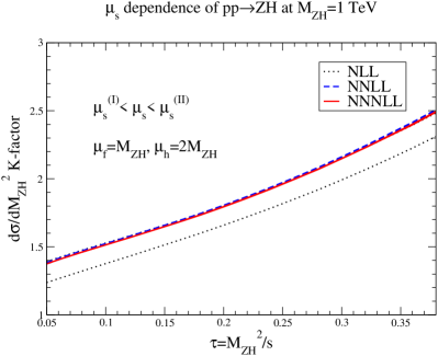
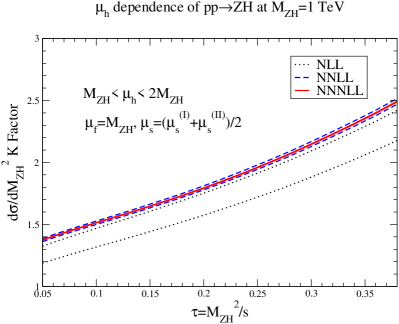
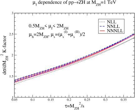
We investigate the numerical effects of the scale variation by plotting the differential cross section of the threshold resummation of Eq. (12) and varying the soft, hard, and factorization scales. It is customary to measure the size of QCD corrections by a -factor () typically defined as the ratio of a higher order cross section to the lowest order cross section:
| (17) |
where is a distribution defined at higher order in QCD.
To study the scale variation arising from threshold resummation, we investigate the -factor of Eq. (17) defined with
| (18) |
To isolate the effects of the scale variation due to threshold resummation from effects of the scale variation due to parton distribution functions (PDFs) and running , the -factor is evaluated by using the NNLO MSTW20008 Martin et al. (2009) PDF set and the -loop value of for all orders of the threshold resummed cross section and the LO cross section. Figure 1 shows the scale variation of this choice of -factor as a function of at NLL between the dotted curves, NNLL between the dashed curves, and NNNLL between the solid curves for production at TeV. The soft scale variation in , with and held constant, is shown in Fig. 1. The variation in the NLL result is significant, but the NNLL and NNNLL curves have little dependence on the soft scale, justifying the choices of . The -factor grows rapidly as increases, as expected. The sensitivity to the hard scale is shown in Fig. 1, with fixed and . The hard scale is set by the invariant mass of the pair, and again we find that at NNLL and NNNLL, there is little dependence on , showing excellent convergence of the perturbation series. Finally, we show the factorization scale dependence in Fig. 1. The factorization scale dependence is small even at NLL.
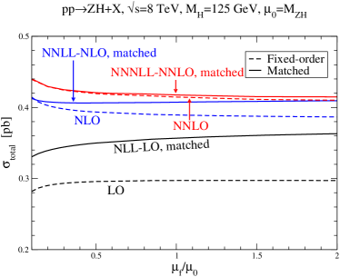
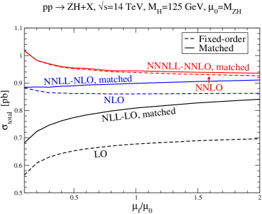
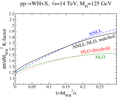
We have also considered the scale dependence of the matched result for the total cross section. Analytic expressions for the LO and NLO fixed order results are found in Refs. Baer et al. (1993); Ohnemus and Stirling (1993); Han and Willenbrock (1991); Brein et al. (2004), and we use the computer code VH@NNLO for the fixed order NNLO results. The matched curves are found using the threshold resummation results of Eq. (13). In Fig. 2, we use the MSTW2008 confidence level PDFs, and use LO PDFs for the LO and the NLL-LO matched curves, NLO PDFs for the NLO and NNLL-NLO matched curves, and NNLO PDFs for the NNLO and NNNLL-NNLO matched curves, and use and -loop evolution of respectively. We include the small contribution from the initial state in the NNLO and NNNLL-NNLO matched curves.
The results for production at TeV and TeV are shown in Figs. 2 and 2, respectively. We have chosen the central scale to be . The top and bottom quark loops from the initial state contribute pb at TeV with . This is the reason for the larger splitting between the NLO and NNLO curves than is seen in the results below. The fixed-order and matched curves have the renormalization/factorization scales set equal, . The matched and resummed curves have the hard scale, , and the soft scale, . The NNNLL-NNLO matched curve is almost identical to the NNLO fixed order curve, and the resummation has little effect at this order. On the other hand, the NNLL-NLO matched curve increases the fixed order NLO result (at ) by about .
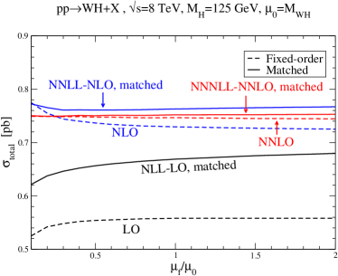
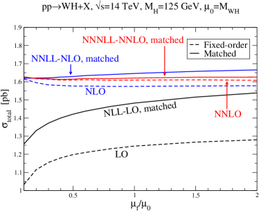
The matched cross sections for production at TeV and 14 TeV are shown in Figs. 2(c) and 2(d). These figures show the sum of and production. As in the case, the NNLO and NNNLL-NNLO matched results for production are quite close and show little scale variation. The NNLL resummation increases the NLO fixed order result by .
The uncertainties in the and cross sections from PDFs, renormalization and factorization scale dependence, and the determination of have been investigated by the LHC Higgs Cross Section Working Group for the NNLO total cross section Dittmaier et al. (2011). They find a total uncertainty at TeV of for and for production for a GeV Higgs boson. Our results show that including the resummation of threshold logarithms to NNNLL accuracy does not induce any further uncertainties. We note that Ref. Dittmaier et al. (2011) also includes the NLO electroweak effects Ciccolini et al. (2003), assuming complete factorization of the QCD and electroweak corrections. In the renormalization scheme, these corrections reduce the total Higgs and vector boson associated rates by about .
IV Kinematic Distributions
IV.1 Transverse-Momentum Distributions
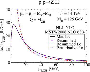
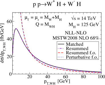
We now give numerical results for the resummed transverse-momentum distributions. The distributions are computed at NLL-NLO accuracy with NLO MSTW2008 confidence level PDFs Martin et al. (2009) and the loop evolution of using the formulae of Appendix A. The numerical results were found by modifying the program HqT2.0 Bozzi et al. (2006); de Florian et al. (2011); HqT . The factorization and renormalization scales are set to the central values of . Also, the resummation scale is set equal to the invariant mass of the vector boson and Higgs pair, i.e., .
Figures 3(a) and 3(b) show the transverse-momentum distribution for and production, respectively, at TeV. The matched transverse-momentum distribution defined by Eqs. (2) and (3) (solid), resummed (dot-dash), fixed order expansion of the resummed (dashed), and fixed-order perturbative (dotted) distributions are shown separately. As expected, the fixed-order expansion of the resummed and perturbative distributions are in good agreement. Hence, the finite piece, defined to be the difference between the perturbative distribution and fixed-order expansion of the resummed distribution as in Eq. (3), is negligible at low transverse momentum and the matched distribution is dominated by the resummed contribution. The transverse-momentum distribution is peaked around GeV for both and production.
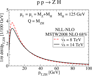
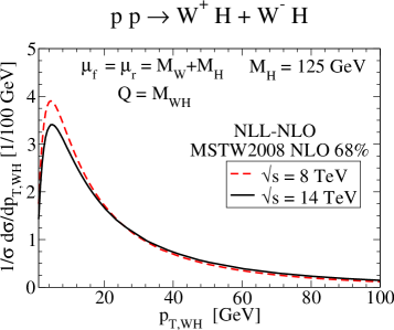
For comparison, in Figs. 3(c) and 3(d) we present the normalized matched transverse-momentum distributions for and production, respectively, at both TeV (dashed) and TeV (solid). The position of the peak of the transverse distribution is not significantly different between the two LHC energies. However, the distribution at TeV has a longer tail than at TeV. This can be understood by noting that higher transverse-momentum events correspond to higher partonic center-of-mass energies. Since events with higher partonic center-of-mass energies are more easily accessible at TeV than at TeV, we would expect there to be larger fraction of high events at TeV than at TeV. Hence, the transverse-momentum distribution has a longer tail for TeV.
Finally, we comment how the transverse-momentum resummation can effect the analysis of kinematical cuts on the signal cross section, particularly in relation to jet vetoes. At hadron machines, the production with Higgs decaying to has large QCD backgrounds. To reduce the backgrounds and effectively trigger on the signal, one usually considers leptonic decays of the vector boson. However, if the vector boson decay contains missing energy, or , semileptonic decays of can be a significant background. Since the background typically has more hard jets than the signal, a jet veto may be applied to suppress this background. We note that vetoing jets with a minimum transverse momentum can be approximated by placing an upper limit on the transverse momentum and, as can be seen in Figs. 3(a) and 3(b), the perturbative calculation is unreliable in this regime. Hence, to fully account for the effects of a jet veto the soft-gluon resummation is needed. There has been much recent work on the systematic resummation of the large logarithms associated with jet vetoes Berger et al. (2011); Banfi et al. (2012a, b); Becher and Neubert (2012); Tackmann et al. (2012).
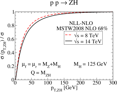
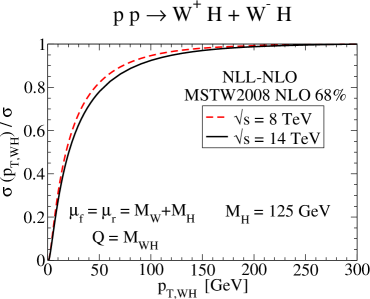
To approximate the effect on the total cross section of a veto on jets with transverse momentum larger than we define
| (19) |
where is the matched transverse-momentum distribution at NLL-NLO in Eqs. (2) and (3). Figure 4 shows this cross section normalized to the total resummed and matched cross section as a function of for (a) and (b) production for both TeV (dashed) and TeV (solid). As noted before in the discussion of Figs. 3(c) and 3(d), at TeV, there is expected to be a larger fraction of high transverse-momentum jets than at TeV. Hence, grows more slowly at TeV than at TeV. From the figures we see that the effects of a () GeV cut decreases the NLO cross section by () and () at TeV and TeV, respectively.
IV.2 Invariant-Mass Distributions
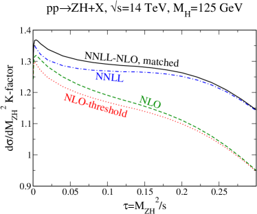
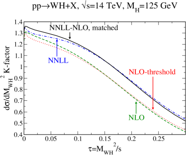
In this section, we give numerical results for the invariant-mass distributions including threshold resummation and matching, using the analytic formulae of Appendix B. Since the distributions vary over many orders of magnitude, it is easier to see the effects in the -factor, as defined in Eq. (17). Figures 5(a) and 5(b) show the -factor versus at NNLL-NLO with for and , respectively. The -factor for the matched result of Eq. (13) is shown with solid lines, the threshold-resummed contribution with dot-dashed lines, the fixed-order perturbative contribution with dashed lines, and the contribution from the leading threshold singularity of the fixed-order perturbative piece with dotted lines. Here we use MSTW2008 confidence level PDFs Martin et al. (2009). The scales are chosen to be , and as in Section III. For the NLO fixed-order result, the leading threshold singularity of the NLO fixed-order result and the threshold-resummed result at NNLL, the NLO PDFs and 2-loop are used, whereas for the LO fixed-order denominator of the -factor, we use the LO PDFs and 1-loop . As expected, the leading singularity and fixed-order results (the two lower curves) are close to each other, since the leading singularity dominates in the fixed-order result. On the other hand, the resummation effect is significant at high , as seen by the large enhancement of the NNLL (the two upper curves) from the NLO result of for both and at .
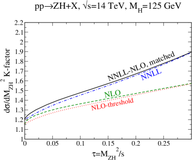
The decrease of the -factor at higher values is due to the PDF effect. To see this, we artificially adopt the NLO MSTW2008 confidence level PDFs and 2-loop for the NLO fixed-order result, the leading threshold singularity of the NLO-fixed-order result and the threshold-resummed result at NNLL, as well as the LO denominator, and show the -factors of these results with for and in Fig. 6(a) and 6(b) respectively. This is to isolate the effects of PDFs from a dynamical origin. The choice of scales is the same as in Fig. 5. We note that the monotonic increase of the -factor distributions in Fig. 6 is drastically different from that in Fig. 5. This demonstrates the importance of a consistent choice of PDFs as in Fig. 5.
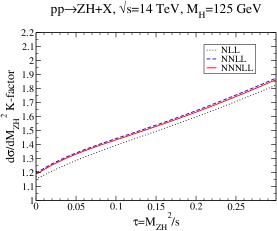
To examine the convergence of the perturbative series, we plot the -factors for the resummed results at NLL, NNLL and NNNLL with TeV for in Fig. 7, using NNLO MSTW2008 confidence level PDFs and 3-loop for all the resummed results as well as the LO denominator. We see from Fig. 7 that the difference between NNLL and NNNLL is tiny (), confirming the excellent convergence of the perturbative series at this order especially after leaving out the PDF effect.
V Conclusions
Given the exciting discovery of a Higgs-like particle at the LHC Gianotti (July 4, 2012); Incandela (July 4, 2012), it becomes imperative to determine its properties. Thus its production rate at the LHC must be calculated as accurately as possible. Since the gauge boson–Higgs associated production is one of the channels that unambiguously probes the coupling with or , it is of particular interest. We combined the long-known fixed-order perturbative QCD calculations for production Brein et al. (2004) with soft-gluon resummation of both threshold logarithms and logarithms which are important at low transverse momentum of the pair.
After a brief overview of the resummation formalism, we carried out detailed numerical analyses at the LHC for TeV and 14 TeV. The overall corrections from NNLO fixed order calculations are sizable, increaing the LO rate by a factor as large as about Dittmaier et al. (2011). After implementing threshold resummation, the dependence of the cross section and various kinematic distributions on the soft and hard scales, as well as on the factorization scale is very weak, indicating the reliability of the calculations. The NNLL threshold resummed total cross section increases the fixed-order NLO result by about , while the NNNLL resummed result has little impact on the NNLO fixed order rate, demonstrating the excellent convergence of the perturbation series.
The transverse-momentum spectrum of the system is calculated via soft and collinear gluon resummation. The distribution is peaked near 5 GeV and the spectrum is slightly harder at the center-of-mass energy of 14 TeV than at 8 TeV. Using the matched transverse-momentum distribution, we have also calculated the effect on the NLO cross section of placing an upper bound on the of the system. Since such an upper bound on the transverse momentum of the system limits the amount of transverse momentum a jet may carry in events, we expect the upper bound on the of the system to approximate a jet veto.
As a final remark, our calculations can be easily extended to other electroweak pair production processes with the same color structures which arise via annihilation at leading order, such as the EW gauge boson pairs and the Higgs pair production and Christensen et al. (2012).
Appendix A: Resummation
In this appendix, we list the functions needed for the resummation of Section II.1 Kodaira and Trentadue (1983, 1982). All formulae in this appendix can be found in Ref. Bozzi et al. (2006), but we include them for the convenience of the reader. First, the coefficients of the QCD beta function are normalized according to the expansion
| (20) |
At LL only the function is needed and the Born level contribution arises only from scatteringBozzi et al. (2006),
| (21) |
and .
Appendix B: Threshold Resummation
In this appendix, we list the functions needed for the threshold resummation of Section 1, taken from Ref. Becher et al. (2008). All formulae in this appendix can be found in Ref. Becher et al. (2008), but we include them for the convenience of the reader.
The running kernel is defined as
| (27) |
where is the anomalous exponent of defined by
| (28) |
and is the Sudakov exponent
| (29) |
The renormalization group equations, Eqs. (28) and (29), can be solved perturbatively. The anomalous dimensions are expanded as
| (30) |
The solutions to Eqs. (28) and (29) are then
| (31) | |||||
and
| (32) | |||||
where .
The cusp anomalous dimension is known to three-loops Korchemskaya and Korchemsky (1992); Moch et al. (2004). The coefficients are
| (33) | |||||
The four-loop coefficient has not yet been calculated, so we use the Padé approximate . The anomalous dimension can be obtained from the partial three-loop on-shell quark form factor Moch et al. (2005). The coefficients are
| (34) | |||||
The final anomalous dimension, , is known from the NNLO calculation of the Altarelli-Parisi splitting function Moch et al. (2004). The coefficients are
| (35) | |||||
The other functions needed are the Wilson coefficient and the soft function . The Wilson coefficient has the expansion,
| (36) |
where , and
| (37) |
This agrees with the corresponding expression in Idilbi et al. (2006).
The soft function to two-loops is
| (38) |
where
| (39) |
This again agrees with the moment-space expression in Idilbi et al. (2006).
Acknowledgements
The work of S.D. and I.L. is supported by the U.S. Department of Energy under grant No. DE-AC02-98CH10886. The work of T.H. is supported in part by the US Department of Energy under grant No. DE-FG02-12ER41832, in part by PITT PACC. The work of A.K.L. and W.K.L. is supported in part by the National Science Foundation under Grant No. PHY-0854782.
References
- Gianotti (July 4, 2012) F. Gianotti, Update on the Standard Model Higgs Searches in ATLAS (July 4, 2012), CERN Seminar.
- Incandela (July 4, 2012) J. Incandela, Update on the Standard Model Higgs Searches in CMS (July 4, 2012), CERN Seminar.
- Glashow et al. (1978) S. Glashow, D. V. Nanopoulos, and A. Yildiz, Phys.Rev. D18, 1724 (1978).
- Stange et al. (1994) A. Stange, W. J. Marciano, and S. Willenbrock, Phys.Rev. D50, 4491 (1994), eprint hep-ph/9404247.
- CDF and Collaborations (2012) CDF and D. Collaborations (Tevatron New Physics Higgs Working Group) (2012), eprint 1207.0449.
- Butterworth et al. (2008) J. M. Butterworth, A. R. Davison, M. Rubin, and G. P. Salam, Phys.Rev.Lett. 100, 242001 (2008), eprint 0802.2470.
- Dittmaier et al. (2011) S. Dittmaier et al. (LHC Higgs Cross Section Working Group) (2011), eprint 1101.0593.
- Dittmaier et al. (2012) S. Dittmaier, C. Mariotti, G. Passarino, R. Tanaka, et al. (2012), eprint 1201.3084.
- Brein et al. (2004) O. Brein, A. Djouadi, and R. Harlander, Phys.Lett. B579, 149 (2004), eprint hep-ph/0307206.
- Brein et al. (2012) O. Brein, R. Harlander, M. Wiesemann, and T. Zirke, Eur.Phys.J. C72, 1868 (2012), eprint 1111.0761.
- Han and Willenbrock (1991) T. Han and S. Willenbrock, Phys.Lett. B273, 167 (1991).
- Baer et al. (1993) H. Baer, B. Bailey, and J. Owens, Phys.Rev. D47, 2730 (1993).
- Ohnemus and Stirling (1993) J. Ohnemus and W. J. Stirling, Phys.Rev. D47, 2722 (1993).
- J.Campbell et al. (2012) J.Campbell, R. Ellis, and C. Williams, MCFM-Monte Carlo for FeMtobarn processes, http://mcfm.fnal.gov/ (2012).
- Collins et al. (1985) J. C. Collins, D. E. Soper, and G. F. Sterman, Nucl.Phys. B250, 199 (1985).
- Sterman (1987) G. F. Sterman, Nucl.Phys. B281, 310 (1987).
- Catani et al. (1996) S. Catani, M. L. Mangano, P. Nason, and L. Trentadue, Nucl.Phys. B478, 273 (1996), eprint hep-ph/9604351.
- Catani and Trentadue (1989) S. Catani and L. Trentadue, Nucl.Phys. B327, 323 (1989).
- Sterman and Vogelsang (2001) G. F. Sterman and W. Vogelsang, JHEP 0102, 016 (2001), eprint hep-ph/0011289.
- Becher et al. (2008) T. Becher, M. Neubert, and G. Xu, JHEP 0807, 030 (2008), eprint 0710.0680.
- Bozzi et al. (2006) G. Bozzi, S. Catani, D. de Florian, and M. Grazzini, Nucl.Phys. B737, 73 (2006), eprint hep-ph/0508068.
- Catani et al. (2001) S. Catani, D. de Florian, and M. Grazzini, Nucl.Phys. B596, 299 (2001), eprint hep-ph/0008184.
- Arnold and Kauffman (1991) P. B. Arnold and R. P. Kauffman, Nucl.Phys. B349, 381 (1991).
- Han et al. (1992) T. Han, R. Meng, and J. Ohnemus, Nucl.Phys. B384, 59 (1992).
- Kulesza et al. (2002) A. Kulesza, G. F. Sterman, and W. Vogelsang, Phys.Rev. D66, 014011 (2002), eprint hep-ph/0202251.
- Parisi and Petronzio (1979) G. Parisi and R. Petronzio, Nucl.Phys. B154, 427 (1979).
- Collins and Soper (1982) J. C. Collins and D. E. Soper, Nucl.Phys. B197, 446 (1982).
- Catani et al. (1993) S. Catani, L. Trentadue, G. Turnock, and B. Webber, Nucl.Phys. B407, 3 (1993).
- Magnea (1991) L. Magnea, Nucl.Phys. B349, 703 (1991).
- Korchemsky and Marchesini (1993) G. Korchemsky and G. Marchesini, Phys.Lett. B313, 433 (1993).
- Bolzoni (2006) P. Bolzoni, Phys.Lett. B643, 325 (2006), eprint hep-ph/0609073.
- Mukherjee and Vogelsang (2006) A. Mukherjee and W. Vogelsang, Phys.Rev. D73, 074005 (2006), eprint hep-ph/0601162.
- Ravindran and Smith (2007) V. Ravindran and J. Smith, Phys.Rev. D76, 114004 (2007), eprint 0708.1689.
- Ravindran et al. (2007) V. Ravindran, J. Smith, and W. van Neerven, Nucl.Phys. B767, 100 (2007), eprint hep-ph/0608308.
- Bauer et al. (2000) C. W. Bauer, S. Fleming, and M. E. Luke, Phys.Rev. D63, 014006 (2000), eprint hep-ph/0005275.
- Bauer et al. (2001) C. W. Bauer, S. Fleming, D. Pirjol, and I. W. Stewart, Phys.Rev. D63, 114020 (2001), eprint hep-ph/0011336.
- Bauer et al. (2002) C. W. Bauer, D. Pirjol, and I. W. Stewart, Phys.Rev. D65, 054022 (2002), eprint hep-ph/0109045.
- Beneke et al. (2002) M. Beneke, A. Chapovsky, M. Diehl, and T. Feldmann, Nucl.Phys. B643, 431 (2002), eprint hep-ph/0206152.
- Bonvini et al. (2012) M. Bonvini, S. Forte, M. Ghezzi, and G. Ridolfi, Nucl.Phys. B861, 337 (2012), eprint 1201.6364.
- Martin et al. (2009) A. Martin, W. Stirling, R. Thorne, and G. Watt, Eur.Phys.J. C63, 189 (2009), eprint 0901.0002.
- Ciccolini et al. (2003) M. Ciccolini, S. Dittmaier, and M. Kramer, Phys.Rev. D68, 073003 (2003), eprint hep-ph/0306234.
- de Florian et al. (2011) D. de Florian, G. Ferrera, M. Grazzini, and D. Tommasini, JHEP 1111, 064 (2011), eprint 1109.2109.
- (43) HqT2.0, http://theory.fi.infn.it/grazzini/codes.html.
- Berger et al. (2011) C. F. Berger, C. Marcantonini, I. W. Stewart, F. J. Tackmann, and W. J. Waalewijn, JHEP 1104, 092 (2011), eprint 1012.4480.
- Banfi et al. (2012a) A. Banfi, G. P. Salam, and G. Zanderighi, JHEP 1206, 159 (2012a), eprint 1203.5773.
- Banfi et al. (2012b) A. Banfi, P. F. Monni, G. P. Salam, and G. Zanderighi (2012b), eprint 1206.4998.
- Becher and Neubert (2012) T. Becher and M. Neubert (2012), eprint 1205.3806.
- Tackmann et al. (2012) F. J. Tackmann, J. R. Walsh, and S. Zuberi (2012), eprint 1206.4312.
- Christensen et al. (2012) N. D. Christensen, T. Han, and T. Li (2012), eprint 1206.5816.
- Kodaira and Trentadue (1983) J. Kodaira and L. Trentadue, Phys.Lett. B123, 335 (1983).
- Kodaira and Trentadue (1982) J. Kodaira and L. Trentadue, Phys.Lett. B112, 66 (1982).
- Ellis et al. (1996) R. K. Ellis, W. J. Stirling, and B. Webber, QCD and collider physics (Cambridge University Press, Cambridge, 1996), and references therein.
- Altarelli et al. (1979) G. Altarelli, R. K. Ellis, and G. Martinelli, Nucl.Phys. B157, 461 (1979).
- de Florian and Grazzini (2001) D. de Florian and M. Grazzini, Nucl.Phys. B616, 247 (2001), eprint hep-ph/0108273.
- Korchemskaya and Korchemsky (1992) I. Korchemskaya and G. Korchemsky, Phys.Lett. B287, 169 (1992).
- Moch et al. (2004) S. Moch, J. Vermaseren, and A. Vogt, Nucl.Phys. B688, 101 (2004), eprint hep-ph/0403192.
- Moch et al. (2005) S. Moch, J. Vermaseren, and A. Vogt, JHEP 0508, 049 (2005), eprint hep-ph/0507039.
- Idilbi et al. (2006) A. Idilbi, X.-d. Ji, and F. Yuan, Nucl.Phys. B753, 42 (2006), eprint hep-ph/0605068.