Non-Fermi Liquid behaviour at the Orbital Ordering Quantum Critical Point in the Two-Orbital Model

Abstract

The critical behaviour of a two-orbital model with degenerate $d_{xz}$ and $d_{yz}$ orbitals is investigated by multidimensional bosonization. We find that the corresponding bosonic theory has an overdamped collective mode with dynamical exponent $z=3$, which appears to be a general feature of a two-orbital model and becomes the dominant fluctuation in the vicinity of the orbital-ordering quantum critical point. Since the very existence of this $z=3$ overdamped collective mode induces non-Fermi liquid behaviour near the quantum critical point, we conclude that a two-orbital model generally has a sizable area in the phase diagram showing non-Fermi liquid behaviour. Furthermore, we show that the bosonic theory resembles the continuous model near the $d$-wave Pomeranchuk instability, suggesting that orbital order in a two-orbital model is identical to nematic order in a continuous model. Our results can be applied to systems with degenerate $d_{xz}$ and $d_{yz}$ orbitals such as iron-based superconductors and bilayer strontium ruthenates Sr₃Ru₂O₇.

1 Introduction

A key puzzle with the iron-pnictide superconductors is one of size: the $0.3\%$ change in the lattice constant at the structural transition is not commensurate with the subsequent massive reorganization in the electronic system as evidenced incommensurate changes are also seen in the Hall and Seebeck coefficients as well as an enhanced tunneling signal at zero-bias in point-contact spectroscopy[1] but most notably by a transport anisotropy that can exceed a factor of two. As such transport anisotropy is difficult to square with standard Fermi liquid behaviour, its mere existence is of great importance as it suggests that non-Fermi liquid behaviour underlies the physics of the pnictides. Since the hunt for non-Fermi liquids is at a nascent stage, a concrete model which is capable of explaining the observed transport anomalies is a pressing problem. In this paper, we propose a concrete model for non-Fermi liquid behaviour in the pnictides which is also capable of capturing the origin of the structural transition.

While on theoretical grounds such physics might be accountable for in the spin sector alone, the pnictides contain an additional orbital degree of freedom which, when present, has been used successfully to explain the discrepancy between the electron transport and the tiny lattice distortion in systems such as the manganites and the ruthenates[2, 3, 4, 5]. The reason is that orbital degrees of freedom are part of the spatial symmetry, not an internal symmetry possessed by the spin sector. Relying on the spin to generate transport anomalies would rest then on the magnitude of the spin-orbit effect on the Fe atom, which is however not sufficient to give rise to such transport anisotropies. The same is true in the ruthenates and the manganites. Further, as is well known from the manganites, coupling fluctuating spins with the lattice can only yield modest changes in the transport properties [6].

We now know from the crucial work of Kugel and Khomskii in the context of multi-orbital Mott systems, that orbital degrees can acquire dynamics and hence can order in a manner identical to $SU(2)$ spins. Orbital ordering, or equivalently orbital polarization, although driven by a small lattice distortion, can yield sizable transport effects in the electronic sector. Based on the success of the orbital ordering program in multi-orbital systems such as the manganites and the ruthenates, one of us[7, 8] as well as others[9, 10, 11, 12] has advocated that similar physics applies to the pnictdes, though not Mott insulators exhibit many of the characteristics of bad metals. In the pnictides, as a result of the $C_{4}$ symmetry in the high-temperature phase, the $d_{xz}$ and $d_{yz}$ orbitals are degenerate. Unequal occupancy of the former two lowers the lattice symmetry to $C_{2}$ and sizable rearrangements obtain in the electronic sector consistent with experiment. For example, two of us have shown[13] using the random-phase approximation that orbital fluctuations between the $d_{xz}$ and $d_{yz}$ orbitals in a five-band model[14] for the pnictides can lead to a break-down of perturbation theory and drive an instability to a non-Fermi liquid state.

In this paper, we approach the problem of the emergence of non-Fermi liquid states of matter using multidimensional bosonization[15, 16, 17, 18]. Since we are after universal physics, rather than the starting from the complexity of a five-band model, we focus just on a two-band model with degenerate $d_{xz}$ and $d_{yz}$ orbitals to see if orbital fluctuations can give rise to non-Fermi liquid behaviour. We establish that as approaching the ferro orbital ordering quantum critical point (FOOQCP), a branch of $z=3$ overdamped collective modes emerges at low energies and small momenta. When these collective modes dominate over the low energy physics at the FOOQCP, electrons are scattered off strongly with them, which leads to a non-Fermi liquid behaviour. This type of non-Fermi liquid behaviour has been well-studied in Hertz-Millis theory[19, 20], and it is the existence of this mode that is the finger print[13, 21, 22, 23, 24] of non-Fermi liquid behaviour associated with the $d$-wave Pomeranchuk instability in continuum and square lattice models. (Due to the existence of $z=3$ overdamped mode, the self-energy of quasi-particle is modified to ${\rm Im\Sigma}\sim\omega^{2/3}$, contrasts to the case of Fermi liquid with ${\rm Im\Sigma}\sim\omega^{2}$.) We show that the emergence of $z=3$ overdamped mode in our system can be obtained analytically and further confirmed by diagonalization of our bosonized Hamiltonian. It should be stressed that the system being studied in this paper is different from [25] because the dispersions for $d_{xz}$ and $d_{yz}$ orbitals do not intersect when interactions are present in our setup.

2 Model Hamiltonian

We wish to describe a two-orbital interacting system. Hence, our starting Hamiltonian contains a kinetic term of the form,

$$H_{t}=\sum_{\vec{k}\sigma}\psi^{\dagger}_{\vec{k}\sigma}[(\epsilon_{+,\vec{k}}-\mu){\mathds{1}}+\epsilon_{-,\vec{k}}\tau_{3}+\epsilon_{xy,\vec{k}}\tau_{1}]\psi_{\vec{k}\sigma},$$ (1)

defined on a square lattice with degenerate $d_{xz}$ and $d_{yz}$ orbitals per site. $\psi^{\dagger}_{\vec{k}\sigma}=(d^{\dagger}_{xz,\sigma}(\vec{k}),d^{\dagger}_{yz,\sigma}(\vec{k}))$ and $d^{\dagger}_{a,\sigma}(\vec{k})$ creates an electron on the orbital $a$ with momentum $\vec{k}$ and spin $\sigma$. $\tau_{i}$ are Pauli matrices. $\epsilon_{+,-,xy}(\vec{k})$ can be obtained by including various hopping parameters which vary from material to material, their explicit expressions are given by

$$\epsilon_{\pm,\vec{k}} =\frac{\epsilon_{x,\vec{k}}+\epsilon_{y,\vec{k}}}{2}$$

$$\epsilon_{x,\vec{k}} =-2t_{1}\cos k_{x}-2t_{2}\cos k_{y}-4t_{3}\cos k_{x}\cos k_{y}$$

$$\epsilon_{y,\vec{k}} =-2t_{2}\cos k_{x}-2t_{1}\cos k_{y}-4t_{3}\cos k_{x}\cos k_{y}$$

$$\epsilon_{xy,\vec{k}} =-4t_{4}\sin k_{x}\sin k_{y}$$ (2)

The definitions of hopping amplitudes $t_{1},t_{2},t_{3}$ and $t_{4}$ are the same as that in [26]. It should be stressed that with numerical values of hopping amplitudes different from [26], the two-orbital model are capable to describe systems other than iron pnictide phenomenologically.

Since we are interested in an orbital ordering instability in the charge channel, only effective inter- and intra-orbital Coulomb interactions are considered here [27]. As a result, the minimal interacting Hamiltonian $H_{I}$ is

$$H_{I}=\sum_{ia}Un_{ia\uparrow}n_{ia\downarrow}+\sum_{i,b>a}\left(U^{\prime}-\frac{J}{2}\right)n_{a}n_{b},$$ (3)

where $U$ and $U^{\prime}$ are the intra- and inter-orbital interactions, and $J$ is Hund’s coupling.

Previously, we used RPA to show that non-Landau damping exists in a 5-band model [13]. To set the stage for the bosonization calculation, we discuss briefly the results of an RPA analysis on the two-band model considered here. We find that the self-energy of the quasiparticle on the Fermi surface shows a non-Fermi liquid behaviour (i.e. ${\rm Im}\Sigma(\vec{k}_{F},\omega)\sim\omega^{\lambda}$ with $\lambda<1$) in the critical region near the orbital ordering quantum critical point (OOQCP). The consistency of this result with our previous 5-band model implies that it is the fluctuations associated with the $d_{xz}$ and $d_{yz}$ orbitals that leads to the non-Fermi liquid behaviour. Moreover, the simplicity of the present two-orbital model allows us to do further analysis on the overdamped $z=3$ mode using a non-perturbative approach, the details of which we now present.

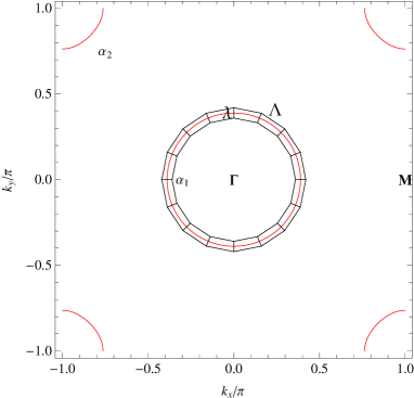
Figure 1: Illustration of the Fermi surface patches used in the multidimensional bosonization. The tight-binding hopping parameters are $t_{1}=-1$, $t_{2}=0.5$, $t_{3}=-0.6$, $t_{4}=-0.5$, and the chemical potential is $\mu=0.5$. There is two disconnected hole pockets, denoted respectively by $\alpha_{1}$ and $\alpha_{2}$, and no electron hole pocket.

3 Multidimensional Bosonization

Multi-dimensional bosonization is ideally suited to this two-band problem because the $d_{xz}$ and $d_{yz}$ bands are quasi-1d. Following the standard procedure[15, 16, 17, 18, 22], we rewrite the tight-binding Hamiltonian in the eigen-band index in order to correctly identify the Fermi surfaces and the interactions between quasiparticles on the Fermi surfaces. Following the same convention used in [28], we introduce a unitary matrix $U_{a\nu,\vec{k}}$ such that the creation operators in the band index can be expressed as $\gamma^{\dagger}_{\nu\sigma\vec{k}}=\psi^{\dagger}_{a\sigma\vec{k}}U_{a\nu,\vec{k}}$, where $\nu$ denotes $\alpha$ (hole) or $\beta$ (electron) Fermi surface. Using the recipe outlined by Haldane, we coarse-grain the Fermi surfaces into $N$ equally sized patches of width $\Lambda$ and thickness $\lambda$, as shown in Fig. 1. We enforce the limit of $\lambda\ll\Lambda\ll k_{F}$ so that the deviation from the multidimensional bosonization due to the processes of momentum-transfer between patches and the effect of curvature within each patch can be significantly reduced[15].

In the limit of low energy and long wavelength, the energy dispersion can be linearized near the Fermi surface, effectively reducing the kinetic term to $H_{t}=\sum_{\vec{k}}\vec{v}_{\vec{k},\nu}\cdot(\vec{k}-\vec{k_{F}})\gamma_{\nu\sigma,\vec{k}}^{\dagger}\gamma_{\nu\sigma,\vec{k}}$. It has been shown[15, 16, 17, 18, 22] that this Hamiltonian can be entirely described by the density fluctuation operator defined as

$$\delta n_{S,\nu\vec{q}}=\sum_{\vec{k},\sigma}(\gamma^{\dagger}_{\vec{k},\nu\sigma}\gamma_{\vec{k}+\vec{q},\nu\sigma}-\delta_{\vec{q},0}n_{\vec{k},\nu\sigma}),$$ (4)

where the summation over momentum is restricted to be within patch $S$. Making use of the special commutation relation between these density fluctuation operators[29], we rewrite the kinetic term as

$$H_{t}=\sum_{S,\nu,\vec{q}}\frac{1}{2N_{\nu}(0)}\delta n_{S,\nu\sigma,-\vec{q}}\delta n_{S,\nu\sigma,\vec{q}},$$ (5)

where $N_{\nu}(0)$ is the density of state at $\nu$ Fermi surface and $\sum_{S}$ represents summation over patches in the limit $N\to\infty$ and $\Lambda\to 0$, which can be changed into line integrals along the Fermi surfaces.

Similarly the interaction Hamiltonian in (3) can be expressed in terms of the density fluctuation operators as well. After a long but straightforward calculation, we arrive at the normal-ordered interaction Hamiltonian,

$$:H_{I}:=\frac{U}{N}\sum_{a,\vec{q},ST\mu\nu}U^{*a\mu}_{\vec{k}_{S}+\vec{q}}U_{\vec{k}_{S}}^{a\mu}\delta n_{S\mu\vec{q}}U^{*a\nu}_{\vec{k}_{T}-\vec{q}}U_{\vec{k}_{T}}^{a\nu}\delta n_{T\nu,-\vec{q}}$$

$$+\frac{\left(2U^{\prime}-J\right)}{N}\sum_{\vec{q}ST\mu\nu,a\neq b}U^{*a\mu}_{\vec{k}_{S}+\vec{q}}U_{\vec{k}_{S}}^{a\mu}\delta n_{S\mu\vec{q}}U^{*b\nu}_{\vec{k}_{T}-\vec{q}}U_{\vec{k}_{T}}^{b\nu}\delta n_{S\nu,-\vec{q}},$$

where the spin index is dropped here after. The Hamiltonian (3) contains forward scattering only, as this is the only relevant interaction for nematic ordering. In general, other types of instabilities may exist and destroy the nematic orbital phase. However, recent Aslamazov-Larkin type vertex correction [30] and renormalization group studies have shown the nematic orbital phase to be stable, thereby justifying our approach [31].

Following [22], we write the effective action for the present bosonic theory, $S=S_{t}+S_{I}$, where

$$S_{t}=-\frac{1}{2}\sum_{S,\nu\sigma,\vec{q}}\int\frac{d\omega}{2\pi}\delta n_{S,\nu\sigma,-\vec{q}}(\chi_{S,\nu}^{0})^{-1}(\vec{q},\omega)\delta n_{S,\nu\sigma,\vec{q}},$$

$$\chi_{S,\nu}^{0}(\vec{q},\omega)=N_{\nu}(0)\vec{v}_{S}\cdot\vec{q}/(\omega-\vec{v}_{S}\cdot\vec{q})$$

$$=N_{\nu}(0)\left(P\frac{\vec{v}_{S}.\hat{q}}{\frac{\omega}{q}-\vec{v}_{S}.\hat{q}}+i\pi\vec{v}_{S}.\hat{q}\delta(\frac{\omega}{q}-\vec{v}_{S}.\hat{q})\right)\ \ \$$ (6)

and

$$S_{I}= \sum_{\vec{q}ST\mu\nu}\int\frac{d\omega}{2\pi}[\frac{U}{N}(\sum_{a}U^{*a\mu}_{\vec{k}_{S}+\vec{q}}U_{\vec{k}_{S}}^{a\mu}U^{*a\nu}_{\vec{k}_{T}-\vec{q}}U_{\vec{k}_{T}}^{a\nu})$$

$$+ \frac{\left(2U^{\prime}-J\right)}{N}(\sum_{a\neq b}U^{*a\mu}_{\vec{k}_{S}+\vec{q}}U_{\vec{k}_{S}}^{a\mu}U^{*b\nu}_{\vec{k}_{T}-\vec{q}}U_{\vec{k}_{T}}^{b\nu})]\delta n_{S\mu,\vec{q}}\delta n_{T\nu,-\vec{q}}.$$

We have introduced a small imaginary part to the denominator of $\chi_{S}^{0}$ to separate it into a real and an imaginary part, which will be helpful for later analysis. One can easily check that the interaction between quasiparticles with $\vec{k}_{S}$ and $\vec{k}_{S}$ is different from that between $\vec{k}_{S}$ and $R\vec{k}_{S}$ ($R\vec{k}_{S}$ denotes the new momentum obtained from rotating $\vec{k}_{S}$ by $\pi/2$). This directly means that the interactions contain both $l=0$ and $l=2$ channels which can be decoupled by introducing the auxiliary fields corresponding to $l$ via Hubbard-Stratonovich transformations as

$$A_{0}(\vec{q}) =\sqrt{\frac{1}{N}}\sum_{\nu,{S_{\nu}}}(c_{\vec{k}_{S_{\nu}}+\vec{q}}c_{\vec{k}_{S_{\nu}}}+s_{\vec{k}_{S_{\nu}}+\vec{q}}s_{\vec{k}_{S_{\nu}}})\delta n_{{S\nu},\vec{q}}$$

$$A_{2}(\vec{q}) =\sqrt{\frac{1}{N}}\sum_{\nu,{S_{\nu}}}\pm(c_{\vec{k}_{S_{\nu}}+\vec{q}}c_{\vec{k}_{S_{\nu}}}-s_{\vec{k}_{S_{\nu}}+\vec{q}}s_{\vec{k}_{S_{\nu}}})\delta n_{{S\nu},\vec{q}},$$ (7)

where $U^{x\beta}_{\vec{k}}=U^{y\alpha}_{\vec{k}}=c_{\vec{k}}$ and $U^{y\beta}_{\vec{k}}=-U^{x\alpha}_{\vec{k}}=s_{\vec{k}}$ and the $+$ and $-$ signs in $A_{2}$ correspond to the $\alpha$ and $\beta$ band respectively and subscripts are added to patch labels to avoid ambiguity. Integrating out the density fluctuation field $\delta n$ leads to an effective action purely in terms of the auxiliary fields.

$$S=\int\frac{d\omega}{2\pi}\sum_{\vec{q}}\begin{pmatrix}A_{0}(-\vec{q})&A_{2}(-\vec{q})\end{pmatrix}\begin{pmatrix}M_{00}&M_{02}\\ M_{20}&M_{22}\\ \end{pmatrix}\begin{pmatrix}A_{0}(\vec{q})\\ A_{2}(\vec{q})\end{pmatrix},$$

where $M_{00}$, $M_{22}$, and $M_{20}$ and $M_{02}$ are given by

$$M_{00}(\vec{q},\omega)= -B^{\prime}+\sum_{\nu,S_{\nu}}\frac{B^{\prime 2}\chi_{S_{\nu}}^{0}}{N}(c_{\vec{k}_{S_{\nu}}+\vec{q}}c_{\vec{k}_{S_{\nu}}}+s_{\vec{k}_{S_{\nu}}+\vec{q}}s_{\vec{k}_{S_{\nu}}})$$

$$\times(c_{\vec{k}_{S_{\nu}}-\vec{q}}c_{\vec{k}_{S_{\nu}}}+s_{\vec{k}_{S_{\nu}}-\vec{q}}s_{\vec{k}_{S_{\nu}}})$$

$$M_{02}(\vec{q},\omega)= \sum_{\nu,S_{\nu}}\frac{BB^{\prime}\chi_{S_{\nu}}^{0}}{N}(c_{\vec{k}_{S_{\nu}}+\vec{q}}c_{\vec{k}_{S_{\nu}}}+s_{\vec{k}_{S_{\nu}}+\vec{q}}s_{\vec{k}_{S_{\nu}}})$$

$$\times(c_{\vec{k}_{S_{\nu}}-\vec{q}}c_{\vec{k}_{S_{\nu}}}-s_{\vec{k}_{S_{\nu}}-\vec{q}}s_{\vec{k}_{S_{\nu}}})$$

$$M_{20}(\vec{q},\omega)= \sum_{\nu,S_{\nu}}\frac{BB^{\prime}\chi_{S_{\nu}}^{0}}{N}(c_{\vec{k}_{S_{\nu}}+\vec{q}}c_{\vec{k}_{S_{\nu}}}-s_{\vec{k}_{S_{\nu}}+\vec{q}}s_{\vec{k}_{S_{\nu}}})$$

$$\times(c_{\vec{k}_{S_{\nu}}-\vec{q}}c_{\vec{k}_{S_{\nu}}}+s_{\vec{k}_{S_{\nu}}-\vec{q}}s_{\vec{k}_{S_{\nu}}})$$

$$M_{22}(\vec{q},\omega)= -B+\sum_{\nu,S_{\nu}}\frac{B^{2}\chi_{S_{\nu}}^{0}}{N}(c_{\vec{k}_{S_{\nu}}+\vec{q}}c_{\vec{k}_{S_{\nu}}}-s_{\vec{k}_{S_{\nu}}+\vec{q}}s_{\vec{k}_{S_{\nu}}})$$

$$\times(c_{\vec{k}_{S_{\nu}}-\vec{q}}c_{\vec{k}_{S_{\nu}}}-s_{\vec{k}_{S_{\nu}}-\vec{q}}s_{\vec{k}_{S_{\nu}}})$$ (8)

and $B=U/2-U^{\prime}+J/2$, $B^{\prime}=U/2+U^{\prime}-J/2$.

It is important to recognize that the $A_{2}(0)$ field is associated with the orbital ordering parameter which breaks the $C_{4}$ symmetry. To see this, one can exploit the unitary matrix $U_{a\nu,\vec{k}}$ to transform $A_{2}(0)$ back to the orbital basis, and the resulting quantity will give the difference between the occupation number of the $yz$ orbital and $xz$ orbitals. As a result, we will focus on the region near OOQCP, that is, $M_{22}(0)\approx 0$, and the collective modes, if any, can be determined by the condition $M_{02}^{2}-M_{00}M_{22}=0$.

To evaluate the OOQCP condition, $M_{22}(0)=0$, we take the limit $\omega/q\to 0$ and then $\vec{q}\to 0$ as advocated previously[22]. As a result, ${\rm Re}\chi_{S}^{0}(0)=-N_{\nu}(0)$, and the condition for the OOQCP is

$$\left(-1+(U-2U^{\prime}+J)\frac{1}{2}\sum_{\nu}N_{\nu}(0)I_{\nu}\right)\geq 0,$$

$$I_{\nu}=-\frac{1}{N}\sum_{S_{\nu}}(c_{\vec{k}_{S_{\nu}}}^{2}-s^{2}_{\vec{k}_{S_{\nu}}})^{2}.$$ (9)

Indeed, our condition for the OOQCP given in (9) is a generalization of the condition for the $d$-wave Pomeranchuk instability, $f_{2}N(0)\leq-1$, in the continuous model[32, 22].

Now we turn to the collective modes in the critical region near the OOQCP. The low energy and long wavelength limit corresponds to $q\to 0$ and $\omega/(q\bar{v}_{S})\to 0$, where $\bar{v}_{S}$ is the average Fermi velocity. A small $q$ expansion on $M_{22}$ gives

$$M_{22}(\vec{q},\omega)=-B+ \sum_{\nu,S_{\nu}}\frac{B^{2}\chi_{S_{\nu}}^{0}(\vec{q},\omega)}{N}\left((c_{\vec{k}_{S_{\nu}}}^{2}-s_{\vec{k}_{S_{\nu}}}^{2})^{2}+\cdots\right)$$

The $q^{2}$ term can be separated into real and imaginary part by the same trick. However, the imaginary part is higher order and can be neglected. Performing a similar analysis on $M_{00}$ and $M_{02}$, one can find that in the small $q$ and $\omega/(q\bar{v}_{S})$ limit,

$$M_{22} =M^{(0)}_{22}+i\frac{\omega}{q}\widetilde{M}^{(0)}_{22}+M^{(2)}_{22}q^{2}+\cdots$$

$$M_{00} =M^{(0)}_{00}+i\frac{\omega}{q}\widetilde{M}^{(0)}_{00}+M^{(2)}_{00}q^{2}+\cdots$$

$$M_{02} =M^{(1)}_{02}q+\cdots,$$ (10)

where

$$M_{22}^{(0)} =-B-\sum_{\nu,S_{\nu}}\frac{B^{2}}{N}(c_{\vec{k}_{S_{\nu}}}^{2}-s_{\vec{k}_{S_{\nu}}}^{2})^{2}N_{\nu}(0)$$

$$\widetilde{M}_{22}^{(0)} =\sum_{\nu}\frac{B^{2}\pi}{N\Lambda}N_{\nu}(0)(c_{\vec{k}_{S_{\nu}}}^{2}-s_{\vec{k}_{S_{\nu}}}^{2})^{2}$$

$$\times\frac{\sqrt{(dk_{y}/dk_{x})^{2}+1}}{(\omega/q-\vec{v}_{S_{\nu}}.\hat{q})^{\prime}}|_{\omega/q=\vec{v}_{S_{\nu}}.\hat{q}}$$

$$M_{22}^{(2)} =-\sum_{\nu,S_{\nu}}\frac{B^{2}}{N}N_{\nu}(0)\Big{(}\frac{1}{2}(c_{\vec{k}_{S_{\nu}}}^{2}-s_{\vec{k}_{S_{\nu}}}^{2})$$

$$\times(c_{\vec{k}_{S_{\nu}}}(\vec{q}.\nabla)^{2}c_{\vec{k}_{S_{\nu}}}+s_{\vec{k}_{S_{\nu}}}(\vec{q}.\nabla)^{2}s_{\vec{k}_{S_{\nu}}})$$

$$-(c_{\vec{k}_{S_{\nu}}}(\vec{q}.\nabla)c_{\vec{k}_{S_{\nu}}}-s_{\vec{k}_{S_{\nu}}}(\vec{q}.\nabla)s_{\vec{k}_{S_{\nu}}})^{2}\Big{)}$$ (11)

where the prime in $\widetilde{M}^{(0)}_{22}$ denotes derivative with respect to $k_{x}$.

Consequently, we find that near the OOQCP (in (10), $M^{(0)}_{22}\approx 0$), the solution to

$$i\frac{\omega_{col}}{q}\widetilde{M}^{(0)}_{22}M^{(0)}_{00}+(M^{(0)}_{00}M^{(2)}_{22}-M^{(1)2}_{20})q^{2}=0$$ (12)

defines the collective $z=3$ overdamped collective mode. This mode has a strong dependence on the Fermi surface topology and momentum $\vec{q}$. In the low-energy limit, $\omega/(q\bar{v}_{S})\to 0$, the condition $\omega/q=\vec{v}_{S}\cdot\hat{q}$ basically requires that $\vec{v}_{S}$ is perpendicular to $\vec{q}$. Therefore, the Fermi surface should be smooth enough such that for an arbitrary direction of $\vec{q}$, there exists at least one perpendicular $\vec{v}_{S}$. This is not always the case, for example when the Fermi surface is a perfect square. For realistic models, $\widetilde{M}^{(0)}_{22}$ is always finite except when $q_{x}=\pm q_{y}$. This obtains because $c_{\vec{k}_{S}}^{2}-s_{\vec{k}_{S}}^{2}$ vanishes when $\vec{k}_{S,x}=\pm\vec{k}_{S,y}$. Therefore, there will be no overdamped modes along the Brillouin zone diagonal, which matches precisely with previous studies of the Pomeranchuk instability on a square lattice[23, 24].

Figure 2: Eigenvalues of the imaginary mode of the bosonized Hamiltonian for $BN_{\alpha_{1}}(0)=-4.344$ and $q_{y}=0$. The black dashed curve is a the fitting with the functional form, $aq_{x}^{3}$. The case of $q_{x}<0.1$ is beyond the numerical accuracy with the choice of 2000 patches. More patches are required to access to the region of smaller $q_{x}$.

It is worth making a comparison between our result and the previous study on a continuous model by Lawler, et. al.[22]. They demonstrated that the $z=3$ overdamped collective mode emerges close to the critical point in the continuum model when an interaction is present in the $l=2$ channel, which is similar to the case of the itinerant ferromagnetic quantum critical point[19, 20]. It is remarkable to see that such an overdamped $z=3$ collective mode exists in our lattice model as well, which strongly suggests that the orbital order in a lattice model is essentially equivalent to the nematic order in a continuous model. Furthermore, the existence of this overdamped $z=3$ collective mode from the non-perturbative multidimensional bosonization technique builds a solid foundation for non-Fermi liquid behaviour since the single-particle Green function is changed fundamentally and obtains a non-perturbative form in the presence of this mode, as shown by Lawler et. al.[22].

4 Numerical Result

The collective modes can also be obtained by performing a generalized Bogoliubov transformation[33] on the bosonized Hamiltonian which allows us to make a direct comparison with the analytic result obtained above. For demonstration purposes, we choose a set of model parameters given in figure. 1 which have two hole pockets $\alpha_{1}$ and $\alpha_{2}$ but no electron pocket.We have just considered the fluctuations on the $\alpha_{1}$ hole Fermi pocket which is sufficient to capture the emergence of the $z=3$ overdamped collective mode. Adding up Eqs. 5 and 3, we obtain the resulting Hamiltonian,

$$H=\frac{1}{N_{\alpha_{1}}(0)}\sum_{ST,\vec{q}}\left(\delta_{S,T}+N_{\alpha_{1}}(0)U_{S,T}(\vec{q})\right)\delta n_{T,-\vec{q}}\delta n_{S,\vec{q}},$$ (13)

where $U_{S,T}(\vec{q})=B/N(c_{\vec{k}_{S}+\vec{q}}c_{\vec{k}_{S}}-s_{\vec{k}_{S}+\vec{q}}s_{\vec{k}_{S}})(c_{\vec{k}_{S}-\vec{q}}c_{\vec{k}_{S}}-s_{\vec{k}_{S}-\vec{q}}s_{\vec{k}_{S}})$. The density fluctuation operator $\delta n$ can be rewritten in terms of bosonic creation and annihilation operators[16, 22]

$$\delta n_{S,-\vec{q}}=\sqrt{\vec{q}\cdot\vec{v}_{S}}a_{S,\vec{q}}\theta[\vec{q}\cdot\vec{v}_{S}]+\sqrt{-\vec{q}\cdot\vec{v}_{S}}a_{S,\vec{q}}^{\dagger}\theta[-\vec{q}\cdot\vec{v}_{S}]$$

$$\delta n_{S,\vec{q}}=\sqrt{-\vec{q}\cdot\vec{v}_{S}}a_{S,\vec{q}}\theta[-\vec{q}\cdot\vec{v}_{S}]+\sqrt{\vec{q}\cdot\vec{v}_{S}}a_{S,\vec{q}}^{\dagger}\theta[\vec{q}\cdot\vec{v}_{S}]$$ (14)

It can be checked that $a$ and $a^{\dagger}$ must satisfy the standard commutation relation for bosons in order to satisfy the unusual commutation relation between $\delta n$[16, 22]. The Hamiltonian can now be rewritten in terms of these bosonic operators and diagonalized with a generalized Bogoliubov transformation.

The diagonalization of the bosonic Hamiltonian is done with 2000 Fermi surface patches and the interaction parameters are set to the values for the OOQCP, $(U-2U^{\prime}+J)N_{\alpha_{1}}(0)=-4.334$. For each momentum $\vec{q}$, we diagonalize a bosonic Hamiltonian with a size of $4000\times 4000$. The energy of the overdamped collective mode can be identified uniquely as the only purely imaginary eigenvalue of the bosonized Hamiltonian for each $\vec{q}$ Fig. 2 plots the magnitude of this purely imaginary eigenvalue $\lambda_{H}$ as a function of $q_{x}$ for $q_{y}=0$, which can be fitted perfectly with a function of the form $aq_{x}^{3}$ (dashed curve). This proves that this branch of the overdamped collective modes indeed has $z=3$. We have also checked another choice of model parameters given by Qi et. al.[28] as a minimal model for iron-based superconductors. In this case, the electron pockets have a much larger density of states than the hole pockets, and we find that the OOQCP is given by $U/4t\approx 1.7$, which is in a reasonable range to be experimentally relevant. We still find the same $z=3$ overdamped collective mode from the technique presented above, which supports our overall conclusion that the overdamped critical mode with $z=3$ is a general feature in a two-orbital model close to the OOQCP.

5 Conclusion

Using non-perturbative multidimensional bosonization, we have demonstrated the emergence of a $z=3$ overdamped collective mode from a general two-orbital model in the vicinity of the orbital ordering quantum critical point. Since it has been well-established that the very existence of a $z=3$ overdamped mode[21, 22, 23, 24] completely washes out the standard Fermi liquid description, non-Fermi liquid behaviour should generally occur in a two-orbital model or in a multiorbital model with degenerate $d_{xz}$ and $d_{yz}$ orbitals. Our bosonic theory provides a solid non-perturbative foundation for the interpretation of the anomalous zero-bias enhancement observed in recent point-contact spectroscopy experiments on a variety of iron-based superconductors[36, 1] as non-Fermi liquid behaviour induced by orbital fluctuations[13].

- [1] Arham H. Z. et al., Phys. Rev. B, 85 (2012) 214515.
- [2] Mackenzie A. P., Bruin J. A. N., Borzi R. A., Rost A. W. and Grigera S. A., Physica C, 481 207 (2012).
- [3] Rost A. W. , Grigera S. A. , Bruin J. A. N., Perry R. S., Tian D., Raghu S., Kivelson S. A. and Mackenzie A. P., Proc. Nat. Acad. Sci., 108 (2011) 16549.
- [4] Raghu S., Paramekanti A., Kim E A., Borzi R. A., Grigera S. A., Mackenzie A. P. and Kivelson S. A., Phys. Rev. B, 79 (2009) 214402.
- [5] Lee W. -C. and Wu, C. Phys. Rev. B, 80 (2009)104438.
- [6] Millis A. J., Littlewood P. B., and Shraiman B. I., Phys. Rev. Lett., 74 (1995) 5144 .
- [7] Lv W., Wu J., and Phillips P., Phys. Rev. B, 80 (2009) 224506 .
- [8] Lv W., Krüger F., and Phillips P., Phys. Rev. B, 82 (2010) 045125 .
- [9] Krüger F., Kumar S., Zaanen J. and van den Brink J., Phys. Rev. B, 79 (2009) 054504.
- [10] Lee C. C., Yin W. G. and Ku W., Phys. Rev. Lett., 103 (2009) 267001.
- [11] Chen C. C., Maciejko J., Sorini A. P., Moritz B., Singh R. R. P. and Devereaux T. P., Phys. Rev. B, 82 (2010) 100504.
- [12] Nevidomskyy A. H., arXiv:1104.1747v1 [cond-mat.str-el].
- [13] Lee W. -C. and Phillips P. W., Phys. Rev. B, 86 (2012) 245113.
- [14] Graser S., Maier T. A., Hirschfeld P. J. and Scalapino D. J., New Journal of Physics, 11 (2009) 025016.
- [15] Haldane F. D. M., Proceedings of the International School of Physics ”Enrico Fermi”, Course CXXI ”Perspectives in Many-Particle Physics,” edited by Broglia R. A. and Schrieffer J. R. (North-Holland, Amsterdam) 1994.
- [16] Castro Neto A. H. and Fradkin E., Phys. Rev. Lett., 72 (1994) 1393.
- [17] Houghton A. and Marston J. B., Phys. Rev. B, 48 (1993) 7790 .
- [18] Houghton A., Kwon H.-J. and Marston J. B., Advances in Physics, 49 (2000) 141.
- [19] Hertz J. A., Phys. Rev. B, 14 (1976) 1165.
- [20] Millis A. J., Phys. Rev. B, 48 (1993) 7183.
- [21] Oganesyan V., Kivelson S. A. and Fradkin E., Phys. Rev. B, 64 (2001) 195109.
- [22] Lawler M. J., Barci D. G., Fernández V., Fradkin E. and Oxman L., Phys. Rev. B, 73 (2006) 085101.
- [23] Metzner W., Rohe D., and Andergassen S., Phys. Rev. Lett., 91 (2003) 066402.
- [24] Dell’Anna L. and Metzner W., Phys. Rev. B, 73 (2006) 045127.
- [25] Mineev V. P. and Michal V. P., arXiv:1206.3468v1 [cond-mat.str-el].
- [26] Raghu, S. and Qi, X. -L. and Liu, C. -X. and Scalapino, D. J. and Zhang, S. -C., Phys. Rev. B, 77 (2008) 220503.
- [27] Onari S. and Kontani H., Phys. Rev. Lett., 109 (2012) 137001.
- [28] Qi X. -L., Raghu S., Liu C. -X., Scalapino D. J. and Zhang S. -C., arXiv:0804.4332 [cond-mat.supr-con].
- [29] Castro Neto A. H. and Fradkin E., Phys. Rev. B, 49 (1994) 10877.
- [30] Ohno Y., Tsuchiizu M., Onari S., and Kontani H., J. Phys. Soc. Jpn., 82 (2013) 013707.
- [31] Tsuchiizu M., Onari S., and Kontani H., arXiv:cond-mat/1209.3664.
- [32] Pomeranchuk I. J., Sov. Phys. JETP, 8 (1958) 361.
- [33] Bogoliubov N. N. and Bogoliubov jr N. N., An Introduction to Quantum Statistical Mechanics, (Gordon and Breach, New York) 1982.
- [34] Pethick C. J. and Smith H., Bose-Einstein Condensation in Dilute Gases, (Cambrige University Press, Cambridge) 2002.
- [35] Shchesnovich, V. S., Physics Letters A, 349 (2006) 398.
- [36] Arham H. Z. et al., arXiv:1108.2749v1 [cond-mat.supr-con].