Detecting sparse cone alternatives for Gaussian random fields, with an application to fMRI

Abstract

Our problem is to find a good approximation to the P-value of the maximum of a random field of test statistics for a cone alternative at each point in a sample of Gaussian random fields. These test statistics have been proposed in the neuroscience literature for the analysis of fMRI data allowing for unknown delay in the hemodynamic response. However the null distribution of the maximum of this 3D random field of test statistics, and hence the threshold used to detect brain activation, was unsolved. To find a solution, we approximate the P-value by the expected Euler characteristic (EC) of the excursion set of the test statistic random field. Our main result is the required EC density, derived using the Gaussian Kinematic Formula.

t1Supported in part by NSF grant DMS-0906801. and t2Keith Worsley, friend, mentor and colleague passed away February 27, 2009.

1 Introduction

It seems appropriate to begin this paper with a tribute to the paper’s second author, Keith Worsley, for whom this appears posthumously. This paper is to appear in a volume celebrating David Siegmund’s 70th birthday. David and Keith Worsley had worked together several times over their careers Siegmund and Worsley (1995); Shafie et al. (2003), most often at the intersection of their two interests: the distribution of the maximum of random fields. While David’s interests range from the smooth to the non-smooth case, Keith was most interested in smooth random fields and their application to brain imaging Worsley (1994); Friston et al. (1995); Worsley et al. (1996). This paper represents Keith Worsley’s last work, before he passed away prematurely from pancreatic cancer in February 2009. Keith and the first author had discussed this paper right up to a few days before he passed away.

David has considered two main approaches to such problems: Weyl’s volume of tube formulas as in Johnstone and Siegmund (1989); Knowles and Siegmund (1989) and change of measure approaches as in Nardi et al. (2008). On the other hand, Keith preferred using the expected Euler characteristic (EC) approach of Adler (1981) and his generalizations Worsley (1995b). In this paper, we combine the EC approach to the volume of tube formula via the Gaussian Kinematic Formula (Taylor, 2006) which expresses Keith’s EC densities in terms of coefficients the Gaussian measure of a tube. Referring back to David Siegmund’s approach to these problems, these coefficients are also coefficients in an expansion of their own change of measure formula on Gaussian space (Taylor and Vadlamani, 2011).

This paper is concerned with the maxima of (functions of) smooth Gaussian random fields. Let $T(s)$, $s\in\mathbb{R}^{D}$ be a random field, and let $S\subset\mathbb{R}^{D}$ be a fixed search region. Our main interest is to find good approximations to the P-value of the maximum of $T(s)$ in $S$:

$$\mathbb{P}\left(\max_{s\in S}T(s)\geq t\right).$$ (1)

The random field $T(s)$ will be one of a variety of test statistics for a cone alternative in a multivariate Gaussian random field. Two of these test statistics have been proposed in the neuroscience literature (Friman et al., 2003; Calhoun et al., 2004) but without a P-value (1). Worsley and Taylor (2006) gives a heuristic approximation to the P-value of the Friman et al. (2003) statistic. This has been incorporated into the R package fMRI (Polzehl and Tabelow, 2006). This paper aims to give a correct P-value approximation to both of these test statistics and the likelihood ratio test statistic.

To do this, we first define the test statistic random fields in Section 2, then evaluate their approximate P-values (1) in Section 3 using the EC heuristic and the Gaussian kinematic formula. Section 3 concludes with a subsection that relates our methods to those we have used for the Hotelling’s $T^{2}$ random field (Taylor and Worsley, 2008). Finally in Section 4 we apply our methods to the re-analysis of an fMRI data set already used for the same purpose in Worsley and Taylor (2006).

2 The test statistics

2.1 Definitions of the test statistics

The test statistics are defined as follows. Let $Z(s)=(Z_{1}(s),\dots,Z_{n}(s))^{\prime}$, $s\in S\subset\mathbb{R}^{D}$, be a vector of $n$ i.i.d. Gaussian random fields with

$$\mathbb{E}(Z(s))=\mu(s),\ \ \ \ \mathbb{V}(Z(s))=\sigma(s)^{2}I_{n\times n}.$$

Usually $\sigma(s)$ is unknown and must be estimated separately at each point, so keeping this in mind, we will set $\sigma(s)=1$ without loss of generality. Let $U\subset O^{n-1}$, the unit $(n-1)$-sphere. At each $s\in S$, we are interested in testing that the mean is zero against the cone alternative:

$$H_{0}:\mu(s)=0\ \ \ \text{vs.}\ \ \ H_{1}:\mu(s)\in\text{Cone}(U)=\{c\cdot u:c\geq 0,\,u\in U\}$$

(Robertson et al., 1988). The likelihood ratio test of $H_{0}$ vs. $H_{1}$ is equivalent to

$$\bar{\chi}(s)=\max_{u\in U}u^{\prime}Z(s),$$ (2)

which we call the $\bar{\chi}$ random field because it has a so-called $\bar{\chi}$ marginal distribution when $\text{Cone}(U)$ is convex (see Section 2.3 below). As mentioned above, $\sigma(s)$ is usually unknown so the $\bar{\chi}$ random field must be normalized separately at every point $s$. We shall consider two ways of doing this.

The first is the likelihood ratio cone random field, equivalent to the likelihood ratio of the cone alternative under unknown variance:

$$T_{\rm LR}(s)=\frac{\bar{\chi}(s)}{\sqrt{(||Z(s)||^{2}-\bar{\chi}(s)^{2})/n}},$$

or equivalently, the maximum correlation between a point in the cone and the data. The second, proposed by Friman et al. (2003), is only defined if $U$ is a subset of some $k$-dimensional subspace of $\mathbb{R}^{n}$, in which case there are effectively $\nu=n-k$ residual degrees of freedom which can be used to estimate $\sigma(s)$ and normalize $\bar{\chi}(s)$. Suppose $Z_{\bot}(s)$ is the projection of $Z(s)$ onto the orthogonal complement of the linear span of $U$, so that $Z_{\bot}(s)$ is independent of $\bar{\chi}(s)$ and has mean 0 under $H_{1}$. Then the independently normalized cone random field is

$$T_{\rm IN}(s)=\frac{\bar{\chi}(s)}{||Z_{\bot}(s)||/\sqrt{\nu}}.$$

Note that if $U=O^{k-1}$ (by this we mean a $(k-1)$-sphere embedded in $\mathbb{R}^{n}$) then the two cone random fields are both equivalent to the F-statistic random field

$$F(s)=\frac{||Z_{\top}(s)||^{2}/k}{||Z_{\bot}(s)||^{2}/\nu}$$

where $Z_{\top}(s)$ is the projection of $Z(s)$ onto the linear subspace spanned by $U$.

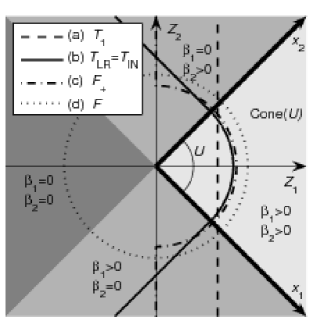
Figure 1: Rejection regions (the side of the boundary that excludes the origin) of the test statistics at $P=0.05$ with infinite sample size for a 2D ($k=2$) right-angled cone alternative covering the first two components $Z_{1},Z_{2}$ of $Z$. The middle of the cone $u$ is parallel to the $Z_{1}$ axis. The cone can also be expressed as a linear model with $m=2$ regressors $x_{1}$ and $x_{2}$ with non-negative coefficients $\beta_{1}\geq 0$ and $\beta_{2}\geq 0$. The $\bar{\chi}$ statistic is the length of the projection of $Z$ onto the nearest edge of the cone (including the vertex of the cone and the interior of the cone itself). The null distribution of $\bar{\chi}$ is a mixture of $\chi_{j}$ random variables with weights $p_{j}={\mathbb{P}}(\#\{\widehat{\beta}{\rm{}^{\prime}s}\geq 0\}=j)$ equal to the relative size of the shaded regions: $p_{0,1,2}=1/4,1/2,1/4$. The statistic $F_{+}$ is the one-sided $F$ statistic of Calhoun et al. (2004).

2.2 Power and maximum likelihood

Both cone statistic random fields should be more powerful than the F-statistic random field since the F-statistic wastes power on alternatives that are outside the cone. The one-sided F-statistic tries to make up for this, but it is inadmissable (for infinite $\nu$ and fixed $s$) because its acceptance region is concave (Birnbaum, 1954) - see Figure 1 - although it is not clear how to construct a test which dominates it. If in fact the alternative is at the middle of the cone then $T_{1}$ should be the most powerful.

Between the two cone statistics, the advantage of $T_{\rm LR}(s)$ is that it uses all the information in the data to estimate the variance and so it should be more powerful than $T_{\rm IN}(s)$. Cohen and Sackrowitz (1993) show that $T_{\rm LR}(s)$ is admissible in specific examples, whereas $T_{\rm IN}(s)$ is always inadmissable. However if in fact the mean is outside the cone but still inside the linear subspace spanned by $U$, then we would expect $T_{\rm IN}(s)$ to be more powerful. The reason is that a mean $\mu(s)$ outside the cone would increase the denominator of $T_{\rm LR}(s)$ but not that of $T_{\rm IN}(s)$. Friman et al. (2003) chose the more conservative $T_{\rm IN}(s)$. This strategy sacrifices a few degrees of freedom and a small loss of power if $\mu(s)$ really is in the cone, against a much larger loss of power if it is not. Worsley and Taylor (2006) investigates power in an fMRI application that we shall also use in Section 4. For a general discussion of power and likelihood ratio tests in this setting see Perlman and Wu (1999).

We note in passing that we have used maximum likelihood principles only at a single point $s$, not over the whole space $S$, which would require a spatial model for the mean and covariance function of the random fields. In the case of known $\sigma(s)$, a standard reproducing kernel argument, discussed in Siegmund and Worsley (1995), can be used to show that if each of the components of $\mu(s)$ is proportional to the spatial correlation function centered at some unknown point $s_{0}$ (which is assumed to be the same for each component), then $\max_{s\in S}\bar{\chi}(s)$ is the likelihood ratio test statistic.

Our interest is confined to $s$ in a search region $S\subset\mathbb{R}^{D}$, where we expect $H_{0}$ to be true at most points, with only a sparse set of points $S_{1}$ where $H_{1}$ is true. This suggests that we should estimate $S_{1}$ by thresholding the above test statistic random fields at some suitably high threshold. Choosing the threshold which controls the P-value of the maximum of the random field to say $\alpha=0.05$ should be powerful at detecting $S_{1}$, while controlling the false positive rate outside $S_{1}$ to something slightly smaller than $\alpha$. Our main problem is therefore to find the P-value of the maximum of these random fields of test statistics (1), which is the main aim of this paper.

2.3 Mixture representation of $\bar{\chi}$

The $\bar{\chi}$ random field is so-named because it has a useful representation in terms of a mixture of $\chi_{j}$ random fields with $j$ degrees of freedom (Lin and Lindsay, 1997; Takemura and Kuriki, 1997). The mixture representation works when $\text{Cone}(U)$ is convex and polyhedral, and asymptotically when $\text{Cone}(U)$ is only locally convex (see Section 3.2 below). The simplest way of seeing where the polyhedral cone enters the picture is to write it as a linear model with non-negative coefficients:

$$H_{1}:\mu(s)=\sum_{j=1}^{m}x_{j}\beta_{j}(s),\ \ \beta_{1}(s),\dots,\beta_{m}(s)\in\mathbb{R}^{+}.$$ (3)

The regressors $x_{1},\dots,x_{m}\in\mathbb{R}^{n}$ contain the vertices of $U$ (times arbitrary scalars), and they may be linearly dependent (see Figure 1). The cone may even contain linear subspaces (for instance, take $x_{2}=-x_{1}$ above) which effectively corresponds to having a certain number of unrestricted coefficients in $\mu(s)$ under $H_{1}$.

To actually compute the $\bar{\chi}(s)$ random field, one must solve a convex problem at each location $s$. This can be done in several ways: the most direct is to first perform all-subsets least-squares regression, then throw out any fitted model that has negative coefficients. Amongst those that are left, the model that fits the best, with fitted values

$$\widehat{Z}(s)=\widehat{\mu}(s)=\sum_{j=1}^{m}x_{j}\widehat{\beta}_{j}(s),\ \ \widehat{\beta}_{1}(s),\dots,\widehat{\beta}_{m}(s)\in\mathbb{R}^{+},$$ (4)

is the maximum likelihood estimator of $\mu(s)$, and $\bar{\chi}(s)=||\widehat{Z}(s)||$. Alternatively, one may solve the problem

$$\mathop{\mathrm{minimize}}_{(\beta(s))_{s\in S}}\sum_{s\in S}\|Z-X\beta(s)\|^{2}_{2}\ \ \text{subject to}\ \ \beta_{i}(s)\geq 0,\ 1\leq i\leq m,s\in S.$$ (5)

This is is a collection of separable convex problems, each of which can be solved via coordinate descent Friedman et al. (2007) or first-order methods (c.f. Becker et al. (2009)). As the inputs are smooth, one would expect that warm starts at adjacent locations would greatly speed up the convergence of such algorithms. There is a huge literature on such non-negative least squares (NNLS) problems, with many applications in inverse problems, and many faster algorithms than all-subsets regression, such as the classic one by Lawson and Hanson (1995).

From a geometric perspective, estimation of $\mu(s)$ is equivalent to projecting $Z(s)$ onto $\text{Cone}(U)$, i.e., finding the face of $\text{Cone}(U)$ closest to $Z(s)$. Here, a face of $\text{Cone}(U)$ could represent the vertex of $\text{Cone}(U)$, in which case $\widehat{Z}(s)=0$; an edge of $\text{Cone}(U)$; or even the interior of $\text{Cone}(U)$, in which case $\widehat{Z}(s)=Z(s)$. Let $A\subset\text{Cone}(U)$ represent a generic face of $\text{Cone}(U)$. Further, let $\widehat{Z}_{A}(s)$ be the projection of $Z(s)$ onto the linear subspace spanned by $A$, so that $\{\widehat{Z}_{A}(s)\in\text{Cone}(U)\}$ is the event that the non-negativity restrictions are satisfied for face $A$. Then,

$$\bar{\chi}(s)=\max_{A}1_{\{\widehat{Z}_{A}(s)\in\text{Cone}(U)\}}\cdot\|\widehat{Z}_{A}(s)\|,$$ (6)

and let $\widehat{A}(s)$ be the value of $A$ that achieves this maximum. Actually, there are values of $Z(s)$ for which more than one face achieves the maximum above, though these occur on lower dimensional subsets of $\mathbb{R}^{n}$, which correspond to lower dimensional surfaces in the search region $S$. From (6), it is clear that

$$\bar{\chi}(s)=\sum_{A}1_{\{\widehat{A}(s)=A\}}\cdot\|\widehat{Z}_{A}(s)\|.$$ (7)

Clearly,

$$\bar{\chi}(s)\bigl{|}\{\widehat{A}(s)=A\}\sim\chi_{\text{dim}(A)},$$

which only depends on the dimensionality of $A$, and so

$$\bar{\chi}(s)\bigl{|}\{\text{dim}(\widehat{A}(s))=j\}\sim\chi_{j}.$$

Hence its unconditional marginal distribution is a mixture of $\chi_{j}$’s

$${\mathbb{P}}(\bar{\chi}(s)\geq t)=\sum_{j=0}^{n}p_{j}(U){\mathbb{P}}(\chi_{j}\geq t)$$ (8)

with weights

$$p_{j}(U)={\mathbb{P}}\left(\text{dim}(\widehat{A}(s))=j\right),\ \ \ \ \ 0\leq j\leq n.$$

These weights are the probability that the face of $\text{Cone}(U)$ that is closest to $Z$ has dimension $j$, or, in terms of the fitted linear model (4),

$$p_{j}(U)={\mathbb{P}}\left(\#\{\widehat{\beta}{\rm{}^{\prime}s}>0\}=j\right),\ \ \ \ \ 0\leq j\leq n.$$

Above, we define $\chi_{0}=0$ to be a constant random variable which corresponds to $Z(s)$ being closest to the vertex of $\text{Cone}(U)$. Depending on the structure of $\text{Cone}(U)$, one or more of the $p_{j}(U)$’s may be zero. More specifically, let $L(U)$ be the largest linear subspace contained in $\text{Cone}(U)$ with $L(U)$ possibly equal to 0, the subspace containing only the 0 vector. It is not hard to see that

$$l(U)\overset{\Delta}{=}\text{dim}(L(U))=\min\{j:p_{j}(U)>0\}$$

and further,

$$\|\widehat{Z}_{L(U)}(s)\|\leq\bar{\chi}(s)\leq\|Z(s)\|.$$

Finally, we also note that, for $t>0$, ${\mathbb{P}}(\chi_{0}\geq t)=0$ so effectively the sum in (8) is really a sum over $1\leq j\leq n$ and we can generally ignore $p_{0}(U)$ which we do in later expressions for the EC densities of $T_{\rm IN}(s)$ and $T_{\rm LR}(s)$.

By approximation, this argument extends to general convex cones, though the $p_{j}$’s have slightly different interpretations even though they are limits of the $p_{j}$’s of the polyhedral approximations, see Section 3.2 below (Lin and Lindsay, 1997; Takemura and Kuriki, 1997).

Note that while the marginal distribution of the $\bar{\chi}(s)$ random field is a mixture of $\chi_{j}$ random variables, it is not strictly a mixture as a random field. Rather, realizations of the random field resemble a patchwork of $\chi_{j}$ random fields with patches $\{s:\widehat{A}(s)=A\}$ on which we observe $\|\widehat{Z}_{A}(s)\|\sim\chi_{{\rm dim}(A)}$ (see Figure 2).

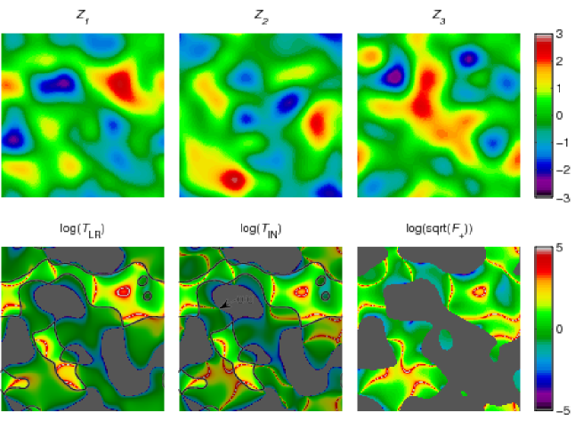
Figure 2: Examples of $n=3$ Gaussian random fields in $D=2$ dimensions (top row). Bottom row: the random fields $T_{\rm LR}$, $T_{\rm IN}$ and $F_{+}$ for the same quarter circle cone as in Figure 1, so that $k=2$ and $\nu=1$. In the three patches the $\bar{\chi}$ random fields are $\chi_{j}$ fields with $j=$ dimensionality of the nearest cone face. In the gray patches, $j=0$, $T_{\rm LR}=T_{\rm IN}=F_{+}=0$; in the medium shaded patches, $j=1$, $T_{\rm LR}^{2}\sim F_{1,2}$ and $T_{\rm IN}^{2}\sim F_{1,1}$; in the unshaded patches, $j=2$, $T_{\rm LR}^{2}=T_{\rm IN}^{2}=F_{+}\sim F_{2,1}$ (times scalars). The boundary between the medium shaded and unshaded patches (heavy black line) is the edge of the cone, $x_{1}$ or $x_{2}$. When the denominator has one degree of freedom, the statistic takes the value $\infty$ on random curves; when it has two degrees of freedom, it takes the value $\infty$ only at the points where these curves touch the boundary. $T_{\rm IN}$ is not defined everywhere because it takes the value 0/0 at random points (arrow).

This representation also sheds some light on the two normalized random fields $T_{\rm LR}(s)$ and $T_{\rm IN}(s)$ as patchwork mixtures of $\sqrt{F}$ random fields of appropriate degrees of freedom. In terms of the representation (7), it is not hard to see that

$$T_{\rm LR}(s)=\sum_{A}1_{\{\widehat{A}(s)=A\}}\cdot\frac{\|\widehat{Z}_{A}(s)\|}{\|Z(s)-\widehat{Z}_{A}(s)\|/\sqrt{n}}.$$ (9)

Above, some slight care must be taken at points $s$ contained in the intersection of the closure of two or more patches. For these points, we can arbitrarily assign $\widehat{A}(s)$ to any appropriate face of $\text{Cone}(U)$. The representation (9) shows immediately that its marginal distribution is that of a mixture of $\sqrt{jn/(n-j)\cdot F_{j,n-j}}$ random variables with weights $p_{j}(U)$. As in the $\chi_{0}$ case, we define $F_{0,l}=0$ to be a constant random variable for all $l$. For the independently normalized cone random field

$$T_{\rm IN}(s)=\sum_{A}1_{\{\widehat{A}(s)=A\}}\cdot\frac{\|\widehat{Z}_{A}(s)\|}{\|Z_{\bot}(s)\|/\sqrt{\nu}}$$ (10)

which shows that its marginal distribution is a mixture of $\sqrt{j\cdot F_{j,\nu}}$ random variables with weights $p_{j}(U)$.

2.4 Dimensionality

The representation of $T_{\rm IN}(s)$ and $T_{\rm LR}(s)$ as patchwork mixtures of $\sqrt{F}$ random fields shows that we must consider constraints on $D$ dictated by the total degrees of freedom $n$ and $\text{Cone}(U)$ (see Figure 2). For the $F$ random field, recalling the argument in Worsley (1994), we note that the set where $||Z(s)||$ takes the value zero is the intersection of the zero sets of each of the components of $Z(s)$, so its dimensionality is $D-n$ if $D\geq n$ or empty if $D<n$. This means that if $D\geq n$ then $F(s)=0/0$ with positive probability somewhere inside $S$, in which case $F(s)$ is not defined. Hence we must have $D<n$ for $F(s)$ to be well defined. The same argument applies to $F_{+}(s)$ and to $T_{1}(s)$ for which we must have $D<\nu+1$.

By a similar argument, $T_{\rm LR}(s)$ is made up of $\sqrt{F_{j,n-j}}$ random fields for $l(U)\leq j\leq n$, so we must have $D<n$ to avoid 0/0 for such random fields. A similar argument applies to $T_{\rm IN}(s)$ though the limit on the dimension is more restrictive and slightly more difficult to describe. In principle, we simply want to avoid 0/0 for the random field $T_{\rm IN}(s)$. However, when $l(U)=0$, we can allow some isolated 0/0 points within the interior of the patch $\{s:\widehat{A}(s)=0\}$, i.e. when the numerator of $T_{\rm IN}(s)$ is 0. If we allow more than isolated points, say curves of 0/0, these will generally intersect the boundary of the patch $\{s:\widehat{A}(s)=0\}$ causing $T_{\rm IN}(s)$ to be undefined at such points (see the white arrows in Figure 2(a,b)). In other words, we really need to avoid 0/0 on the closure of the set $\{s:\widehat{A}(s)\neq 0\}$. When $l(U)=0$, on this set

$$\min\{\|\widehat{Z}_{A}(s)\|:\text{dim}(A)=1\}\leq\bar{\chi}(s)\leq\|Z(s)\|$$

therefore there will be no 0/0’s if there are no 0/0’s for any of the $F_{1,\nu}$ random fields

$$\left\{\frac{\|\widehat{Z}_{A}(s)\|^{2}}{\|Z_{\bot}(s)\|^{2}/\nu}:\text{dim}(A)=1\right\},$$

that is, if $D<\nu+1$. However, if $l(U)>0$, then $\{s:\widehat{A}(s)=0\}$ is of strictly lower dimension than $D$ and even isolated 0/0 points within this patch will cause $T_{\rm IN}(s)$ to be undefined, hence we must again avoid 0/0’s in the closure of $\{s:\widehat{A}(s)\neq 0\}$ which is just $S$, the entire search region. As noted in the previous section, when $l(U)>0$

$$\|\widehat{Z}_{L(U)}(s)\|\leq\bar{\chi}(s)\leq\|Z(s)\|$$

and there will be no 0/0’s in $T_{\rm IN}(s)$ if there are no 0/0’s in the $F_{l(U),\nu}$ random field

$$\frac{\|\widehat{Z}_{L(U)}(s)\|^{2}/l(U)}{\|Z_{\bot}(s)\|^{2}/\nu},$$

that is, if $D<\nu+l(U)$. In summary, considering both cases $l(U)=0$ and $l(U)>0$, we must have $D<\nu+\max(l(U),1)$.

When $\text{Cone}(U)$ is non-convex, the situation is more difficult to describe in exact terms for both $T_{\rm IN}(s)$ and $T_{\rm LR}(s)$. If $\text{Cone}(U)$ is non-convex, then the marginal distribution of $\bar{\chi}(s)$ is no longer exactly a mixture of $\chi_{j}$’s with the error being exponentially small Taylor et al. (2005).

3 P-value of the maximum of a random field

A very accurate approximation to the P-value of the maximum of any smooth isotropic random field $T(s)$, $s\in S\subset\mathbb{R}^{D}$, at high thresholds $t$, is the expected Euler characteristic (EC) $\varphi$ of the excursion set:

$${\mathbb{P}}\left(\max_{s\in S}T(s)\geq t\right)\approx{\mathbb{E}}(\varphi\{s\in S:T(s)\geq t\})=\sum_{d=0}^{D}{\cal L}_{d}(S)\rho_{d}(t),$$ (11)

where ${\cal L}_{d}(S)$ is the $d$-dimensional intrinsic volume of $S$ (defined in Appendix A), and $\rho_{d}(t)$ is the $d$-dimensional EC density of the random field above $t$ (Adler, 1981; Worsley, 1995a; Adler, 2000; Adler and Taylor, 2007). The heuristic is that for high thresholds the EC takes the value 0 or 1 if the excursion set is empty or not, so that the expected EC approximates the P-value of the maximum (see Figure 3). The approximation is extraordinarily accurate, giving exponential accuracy for Gaussian random fields (Taylor et al., 2005). A different approach using volumes of tubes (Knowles and Siegmund, 1989; Johansen and Johnstone, 1990; Sun, 1993; Sun and Loader, 1994; Sun et al., 2000; Pilla, 2006) is, in our context, essentially the same as the methods used here, as shown by Takemura and Kuriki (2002).

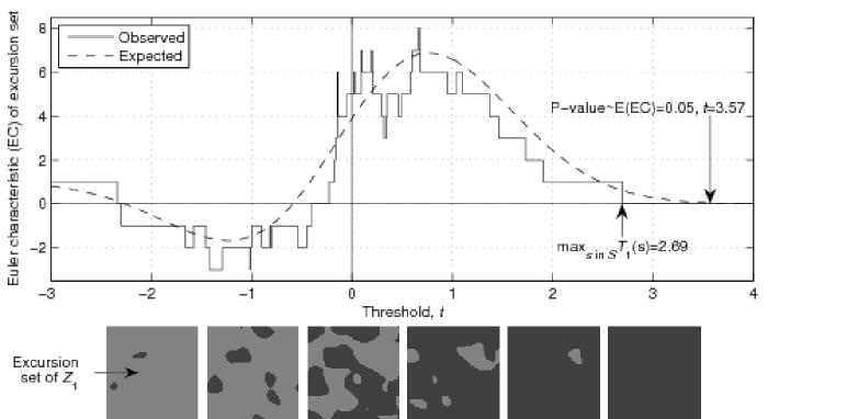
Figure 3: The Euler characteristic (EC) of excursion sets of the Gaussian random field $Z_{1}$ from Figure 2 plotted against threshold $t$, together with the expected EC under $H_{0}$ from (11). Bottom row: the excursion sets (light gray) for $t=-2,\dots,3$; the search region $S$ is the whole image. At high thresholds the expected EC is a good approximation to the P-value of the maximum (arrowed). The approximate $P=0.05$ threshold is $t=3.57$ (arrowed).

For $D=3$, our main interest in applications, ${\cal L}_{0,1,2,3}(S)$ are: the EC, twice the ‘caliper diameter’, half the surface area, and the volume of $S$ respectively (for a convex set, the caliper diameter is the average distance between the two parallel tangent planes to the set). If the random field $T(s)$ is a function of Gaussian random fields, such as all the test statistic random fields considered so far, and these Gaussian random fields are non-isotropic, then it is only necessary to replace intrinsic volume in (11) by Lipschitz-Killing curvature. Lipschitz-Killing curvature depends on the local spatial correlation of the component Gaussian random fields, as well as the search region $S$ (Taylor and Adler, 2003; Taylor and Worsley, 2007).

Morse theory can be used to obtain the EC density of a smooth random field $T=T(s)$ as

$$\rho_{d}(t)={\mathbb{E}}\left(1_{\{T\geq t\}}{\rm det}(-\ddot{T}_{d})\ |\ \dot{T}_{d}=0\right){\mathbb{P}}(\dot{T}_{d}=0),$$ (12)

where dot notation with subscript $d$ denotes differentiation with respect to the first $d$ components of $s$ (Worsley, 1995a). For $d=0$, $\rho_{0}(t)={\mathbb{P}}(T\geq t)$. The Morse method of obtaining EC densities, though straightforward in principle, usually involves an enormous amount of tedious algebra. Entire papers have been devoted to evaluating (12) for an ever wider class of random fields of test statistics such as Gaussian (Adler, 1981), $\chi^{2}$, $T$, $F$ (Worsley, 1994), Hotelling’s $T^{2}$ (Cao and Worsley, 1999b), correlation Cao and Worsley (1999a), scale space (Siegmund and Worsley, 1995; Worsley, 2001; Shafie et al., 2003) and Wilks’s $\Lambda$ (Carbonell and Worsley, 2007). A much simpler method is given in the next section.

3.1 The Gaussian Kinematic Formula

There is a much simpler way of getting EC densities when $T$ is built from independent unit Gaussian random fields (UGRF). A UGRF is a Gaussian random field with zero mean, unit variance, and identity variance of its spatial derivative. Note that any stationary Gaussian random field can be transformed to a UGRF by appropriate linear transformations of its domain and range. Without loss of generality we shall assume that all the random fields considered so far are built from UGRFs.

This simpler method is based on the Gaussian Kinematic Formula discovered by Taylor (2006). The idea is to take the Steiner-Weyl volume of tubes formula (24) and replace the search region by the rejection region, and volume by probability. Somewhat miraculously, the coefficients of powers of the tube radius are (to within a constant) the EC densities we seek.

The details are as follows. Suppose $T(s)=f(Z(s))$ is a function of UGRFs $Z(s)=(Z_{1}(s),\dots,Z_{n}(s))^{\prime}$. Put a tube of radius $r$ about the rejection region $R_{t}=\{z\in\mathbb{R}^{n}:f(z)\geq t\}\subset\mathbb{R}^{n}$, evaluate the probability content of the tube (using the ${\rm N}_{n}(0,I_{n\times n})$ distribution of $Z=Z(s)$), and expand as a formal power series in $r$. Denoting the tube by ${\rm Tube}(R_{t},r)=\{x:\min_{z\in R_{t}}||z-x||\leq r\}$, then

$${\mathbb{P}}\left(Z\in{\rm Tube}(R_{t},r)\right)=\sum_{d=0}^{\infty}\frac{r^{d}}{d!}(2\pi)^{d/2}\rho_{d}(t).$$ (13)

Since the spatial dependence on $s$ is no longer needed, we omit it until further notice.

For example, let $f(z)=u^{\prime}z$ for fixed $u$ with $||u||=1$ so that $T$ is a UGRF. Without loss of generality we can assume that $n=1$ and hence $f(z)=z$. It is easy to see that $R_{t}=[t,+\infty)$ and further

$${\rm Tube}(R_{t},r)=[t-r,+\infty)=R_{t-r}.$$

This observation leads directly to the EC density of the Gaussian random field

$$\rho_{d}^{\rm G}(t)=\left(\frac{-1}{\sqrt{2\pi}}\frac{\partial}{\partial t}\right)^{d}{\mathbb{P}}(T\geq t).$$ (14)

We shall exploit this observation, that the tube is another rejection region but with a lower threshold, to derive the EC density for the $\bar{\chi}$ random field in the next section.

3.2 The $\bar{\chi}$ random field

Now let $R_{t}\subset\mathbb{R}^{n}$ be the rejection region for the $\bar{\chi}$ random field at level $t$. This rejection region is the union of half planes all a distance $t$ from the origin. It is clear that a tube of radius $r$ about such a rejection region is simply another union of half planes all a distance $t-r$ from the origin (provided $r<t$). We thus arrive at precisely the same expression as for the Gaussian case: ${\rm Tube}(R_{t},r)=R_{t-r}$. In exactly the same way, this leads directly to the following representation for the EC densities of a $\bar{\chi}$ random field:

$$\rho_{d}^{\rm\bar{\chi}}(t)=\left(\frac{-1}{\sqrt{2\pi}}\frac{\partial}{\partial t}\right)^{d}{\mathbb{P}}(\bar{\chi}\geq t).$$ (15)

We can now use the mixture representation (8) to show that the EC density of $\bar{\chi}$ is the same mixture of EC densities of the $\chi_{j}$ random field. To see this, note that, by setting $U=O^{j-1}$ in (15), the EC density of $\chi_{j}$ is

$$\rho_{d}^{\chi}(t;j)=\left(\frac{-1}{\sqrt{2\pi}}\frac{\partial}{\partial t}\right)^{d}{\mathbb{P}}(\chi_{j}\geq t).$$ (16)

Combining this with (15) and (8) leads to the first expression of the following Theorem.

Theorem 1.

If $\text{Cone}(U)$ is convex then the EC density of the $\bar{\chi}$ random field is

$$\rho_{d}^{\bar{\chi}}(t)=\sum_{j=1}^{n}p_{j}(U)\rho_{d}^{\chi}(t;j)=\sum_{j=0}^{n-1}{\cal L}_{j}(U)\rho^{G}_{d+j}(t)$$

where $\rho_{d}^{\chi}(t;j)$ and $\rho_{d}^{\rm G}(t)$ are the EC densities of the the $\chi_{j}$ random field (16) and Gaussian random field (14), respectively.

The second part of the Theorem is proved as follows. Another way of evaluating ${\mathbb{P}}(\bar{\chi}\geq t)$ is to note that $u^{\prime}Z$, as a function of $u$, is a UGRF and that $\bar{\chi}$ is its maximum over $U$. Hence we can use the approximation (11) for Gaussian random fields, replacing $S$ by $U$. This is exact for $t>0$ when $\text{Cone}(U)$ is convex. The reason is that the excursion set $\{u\in U:u^{\prime}Z\geq t\}$ generates a cone that is the intersection of a convex circular cone (provided $t>0$) with convex $\text{Cone}(U)$, which is again convex. The EC of $\{u\in U:u^{\prime}Z\geq t\}$ is either 0 or 1 if it is empty or not, that is, if $\bar{\chi}$ is less than or greater than $t$. Hence the expected EC is the P-value, so that (11) is exact and gives

$${\mathbb{P}}(\bar{\chi}\geq t)=\sum_{j=0}^{n-1}{\cal L}_{j}(U)\rho^{G}_{j}(t).$$ (17)

Combining this with (15) yields the second expression of Theorem 1. Note that the weights $p_{j}(U)$ can now be expressed in terms of intrinsic volumes by equating (17) to (8) to give

$$p_{j}(U)=\frac{1}{2^{j}\pi^{\frac{j-1}{2}}\Gamma(\frac{j+1}{2})}\sum_{m=0}^{\lfloor(n-j)/2\rfloor}\frac{(-1)^{m}(d+2m)!}{(4\pi)^{m}m!}{\cal L}_{j+2m-1}(U)$$

(see Chapter 15 in Adler and Taylor (2007)).

Remark 1: If $\text{Cone}(U)$ is not convex, the above argument used to derive (17) fails, though (15) still holds for the coefficients in the exact tube expansion, in the sense that ${\rm Tube}(R_{t},r)=R_{t-r}$. However, if $\text{Cone}(U)$ is locally convex (17) is exponentially accurate Taylor et al. (2005) and therefore the right hand side of the result in Theorem 1 is the EC density up to an exponentially small error.

Remark 2: The representation (7) represents $\bar{\chi}(s)$ (reinstating dependence on $s$) as a mixture of $\chi_{j}(s)$ random fields with weights $p_{j}(U)$. It is therefore not surprising that the EC density of the $\bar{\chi}(s)$ random field is a mixture of the EC densities of $\chi_{j}(s)$ random fields with the same weights. We give a sketch of a proof why this should be so for the simplest cone: the positive orthant in $\mathbb{R}^{k}$

$$\bar{\chi}(s)^{2}=\sum_{j=1}^{k}1_{\{Z_{j}(s)>0\}}Z_{j}(s)^{2}.$$

For this cone, a face is determined by a subset of $\{1,\dots,k\}$ which are the set of non-negative components of $\widehat{\mu}(s)$. It is not hard to see that $\widehat{A}(s)=\{j:Z_{j}(s)<0\}^{c}$ with the empty set representing the vertex of the cone. We shall now make use of Morse theory, which shows that the EC of a set is determined by the critical points of a twice differentiable Morse function defined on the set (Adler, 1981). The Morse theory expression for the EC density (12) is obtained by using the random field itself as the Morse function (Worsley, 1995a). The random field $\bar{\chi}(s)$ as a Morse function is actually differentiable (though not twice differentiable) and it is not hard to show that its critical points are almost surely contained in the interior of the patches. This is because the critical points on the boundary are points where a particular $\chi_{j}(s)$ random field has a critical point and one or more components are 0 (see Figure 2). For instance, critical points that appear on the segment of boundary of the intersection of $\{s:Z_{1}(s)=0\}$ and the patch $\{s:\widehat{A}(s)=\emptyset\}$ are points where $Z_{1}(s)$ has a critical point and $Z_{1}(s)=0$. The number of such points is almost surely 0. Because there are no critical points on the boundary of the patches, we can redefine $\bar{\chi}(s)$ near these boundaries to get a Morse function with the same critical points as $\bar{\chi}(s)$ and the standard Morse-theoretic computation of the expected EC now shows that for each patch $J\subset\{1,\dots,k\}$ we must find the number of critical points of $\chi_{J}(s)^{2}=\sum_{j\in J}Z_{j}^{2}(s)$ above the level $t$, counting multiplicities. The expected EC above the level $t$, similar to (12) will therefore be

$$\sum_{J\subset\{1,\dots,N\}}{\mathbb{E}}\left(1_{\{\widehat{A}(s)=J\}}1_{\{\chi_{J}(s)>t\}}{\rm det}(-\ddot{\chi}_{J,d}(s))\ |\ \dot{\chi}_{J,d}(s)=0\right){\mathbb{P}}(\dot{\chi}_{J,d}(s)=0).$$

Noting that the conditional distribution of $\ddot{\chi}_{J,d}(s)$ given $(Z(s),\dot{Z}(s))$ depends on $Z(s)$ only through $\|Z_{J}(s)\|$ implies that $\ddot{\chi}_{J,d}(s)$ and $1_{\{\widehat{A}(s)=J\}}$ are conditionally independent given $(Z(s),\dot{Z}(s))$. In fact, this also implies that they are actually unconditionally independent. This completes the sketch of the proof: the sum over all subsets $J$ of size $j$ yields $p_{j}(U)$ times the EC densities of $\chi^{2}_{j}$ random fields from (12). To go from the $\bar{\chi}(s)$ to the $T_{\rm IN}(s)$ or $T_{\rm LR}(s)$ random field is not complicated: simply replace $\chi_{J}$ above by the appropriate $F$ random fields in the decomposition (9) or (10), though the conditional independence argument is just slightly more complicated. In the following sections, we prefer to use the Gaussian kinematic formula to give a more direct and complete proof which does not refer to Morse theory and counting critical points.

3.3 The F- and T-statistic random fields

Our main results, stated in Theorem 2 and Theorem 3, are based on a simple refinement of Theorem 1 in which we incorporate a $\chi^{2}$ field in the denominator. To see how it works, let us use the Gaussian kinematic formula to derive the EC density of the F-statistic field. Let $R_{t}\subset\mathbb{R}^{n}$ be the rejection region of the F-statistic random field $F$ with $k,\nu$ degrees of freedom. Without loss of generality, setting $z=(z_{1},\dots,z_{n})$, we can take

$$f(z)=\frac{\sum_{i=1}^{k}z_{i}^{2}/k}{\sum_{i=k+1}^{n}z_{i}^{2}/\nu}.$$

Then, a little elementary geometry (see Figure 4) shows that

$${\mathbb{P}}\left(Z\in{\rm Tube}(R_{t},r)\right)={\mathbb{P}}(\chi_{k}\geq T_{r})+O(r^{n})$$ (18)

where

$$T_{r}=\chi_{\nu}\sqrt{\frac{tk}{\nu}}-r\sqrt{1+\frac{tk}{\nu}}.$$

The remainder above reflects the fact that the tube ${\rm Tube}(R_{t},r)$ is almost equal to the event $\{\chi_{k}\geq T_{r}\}$. Near the origin, this fails but the probability content of where this fails is of order $O(r^{n})$. Further, the EC densities of $F$ are only defined for $d\leq D<n$ (as explained in Section 2.4). Continuing with the main term in (18), and making use of (14),

$${\mathbb{P}}(\chi_{k}\geq T_{r}) ={\mathbb{E}}\left({\mathbb{P}}\left(\chi_{k}\geq T_{r}\ \biggl{|}\chi_{\nu}\right)\right)$$ (19)

$$={\mathbb{E}}\left(\sum_{j=0}^{k-1}{\cal L}_{j}(O^{k-1})\;\rho^{G}_{j}(T_{r})\right)$$

$$=\sum_{d=0}^{\infty}\frac{(2\pi)^{d/2}r^{d}}{d!}\left(1+\frac{tk}{\nu}\right)^{d/2}\sum_{j=0}^{k-1}{\cal L}_{j}(O^{k-1})\;{\mathbb{E}}\left(\rho^{G}_{j+d}\left(\chi_{\nu}\sqrt{\frac{tk}{\nu}}\right)\right).$$

Hence, the EC densities for an F-statistic random field with $k,\nu$ degrees of freedom are given by

$$\rho^{\rm F}_{d}(t;k,\nu)=\left(1+\frac{tk}{\nu}\right)^{d/2}\sum_{j=0}^{k-1}{\cal L}_{j}(O^{k-1})\;{\mathbb{E}}\left(\rho^{G}_{j+d}\left(\chi_{\nu}\sqrt{\frac{tk}{\nu}}\right)\right).$$ (20)

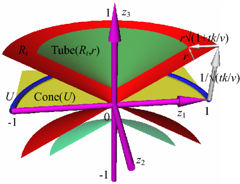
Figure 4: Rejection region $R_{t}$ of the F statistic $F=(z_{1}^{2}+z_{2}^{2})/2/z_{3}^{2}$ with $k=2$ and $\nu=1$. The purple axes are from -1 to 1. The cone generator $U$ is blue, $\text{Cone}(U)$ is transparent yellow. The rejection region for a threshold of $t=3/2$ is red; the tube about the rejection region (radius $r=0.15$) is transparent green. Both rejection region and tube are cut at $z_{2}\geq 0$ and $|z_{3}|\leq 1/\sqrt{3}$. We expand the probability of this tube as a power series in $r$; its coefficients are the EC densities we seek.

For the T-statistic random field $T_{1}$, a similar argument to that leading to (18) shows that we must expand the following probability in a power series:

$${\mathbb{P}}\left(Z_{1}\geq\chi_{\nu}\sqrt{\frac{t^{2}}{\nu}}-r\sqrt{1+\frac{t^{2}}{\nu}}\right)$$

where $Z_{1}\sim N(0,1)$ is independent of $\chi_{\nu}$. In the above expression, $t^{2}$ appears instead of $t$ because $T_{1}^{2}$ is an $F_{1,\nu}$ random field and $Z_{1}$ appears rather than $\chi_{1}=|Z_{1}|$ on the left hand of the inequality side because $T_{1}$ is one-sided. Similar calculations to those above for the F-statistic yield the following expression for the EC densities of the T-statstic random field

$$\rho^{\rm T}_{d}(t;\nu) =\left(1+\frac{t^{2}}{\nu}\right)^{d/2}{\mathbb{E}}\left(\rho^{G}_{d}\left(\chi_{\nu}\sqrt{\frac{t^{2}}{\nu}}\right)\right)$$

$$=\sum_{l=0}^{\lfloor\frac{d-1}{2}\rfloor}\frac{(-1)^{l}(d-1)!\Gamma\left(\frac{d-1-2l+\nu}{2}\right)}{\pi^{(d+1)/2}2^{2l+1}(d-1-2l)!l!\Gamma\left(\frac{\nu}{2}\right)}\left(\frac{t^{2}}{\nu}\right)^{(d-1-2l)/2}\left(1+\frac{t^{2}}{\nu}\right)^{-(\nu-1-2l)/2}$$

for $d>0$ and $\mathbb{P}(T_{1}>t)$ for $d=0$. This is simpler than the expression in Worsley (1994); it is a single sum, whereas the the expression in Worsley (1994) is a double sum.

A simple rearrangement of (20) yields the following equivalent representation of the EC densities of the F-statistic random field in terms of the EC densities of the T-statstic random field:

$$\rho^{\rm F}_{d}(t;k,\nu)=\left(1+\frac{tk}{\nu}\right)^{-d/2}\sum_{j=0}^{k-1}{\cal L}_{j}(O^{k-1})\;\rho^{\rm T}_{d+j}(\sqrt{tk};\nu).$$

3.4 The independently normalized cone random field $T_{\rm IN}$

It is slightly easier to work with $T_{\rm IN}$, since it more closely resembles $F$, so we tackle this ahead of $T_{\rm LR}$. It should now be clear how to proceed: find the rejection region as a function of the $n$ UGRF’s; put a tube around with radius $r$; work out the probability content; differentiate $d$ times to get the EC density. This sounds formidable, but it is in fact virtually identical to the case of the F-statistic presented above. For readers with good geometric intuition, Figure 5 might help: it shows the simple case of the rejection region $R_{t}=\{Z:T_{\rm IN}\geq t\}$ where $k=2$ and $\nu=1$, and $U$ is a quarter circle, as in Figure 2.

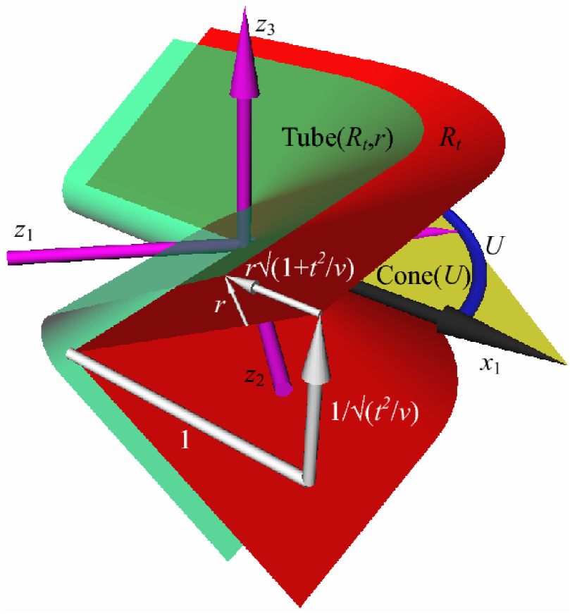
Figure 5: Rejection region $R_{t}$ of the independently normalized test statistic $T_{\rm IN}$ for the same cone as in Figure 2 and the same $z$ as in Figure 4. The cone edges $x_{1}$ and $x_{2}$ are black. The threshold is $t=\sqrt{3}$ and both the rejection region and tube are cut at $z_{1}\pm z_{2}\geq-\sqrt{2}$ and $|z_{3}|\leq 1/\sqrt{3}$.

Theorem 2.

If $\text{Cone}(U)$ is convex then the EC density of the independently normalized cone random field $T_{\rm IN}$ is

$$\rho_{d}^{\rm IN}(t)=\sum_{j=1}^{k}p_{j}(U)\rho_{d}^{\rm F}\left(\frac{t^{2}}{j};j,\nu\right)=\sum_{j=0}^{k-1}{\cal L}_{j}(U)\rho_{d+j}^{\rm T}(t;\nu)\left(1+\frac{t^{2}}{\nu}\right)^{-j/2}.$$

The EC densities are valid for $d<\nu+\max(l(U),1)$, where $l(U)$ is the dimension of the largest linear subspace in $\text{Cone}(U)$.

Remark: The representation (10) represents $T_{\rm IN}$ as a patchwork mixture of $\sqrt{j\cdot F_{j,\nu}}$ random fields with weights $p_{j}(U)$. See Remark 2 after Theorem 1 for why Theorem 2 should not be surprising. For the case of non-convex $\text{Cone}(U)$, see Remark 1 after Theorem 1.

Proof: The same geometric argument that led to (18) leads to the following approximate equality

$$\left\{Z\in{\rm Tube}(R_{t},r)\right\}\simeq\left\{\bar{\chi}\geq T_{r}^{*}\right\}\\$$

where

$$T_{r}^{*}=\chi_{\nu}\sqrt{\frac{t^{2}}{\nu}}-r\sqrt{1+\frac{t^{2}}{\nu}}.$$

In fact, $\{Z\in{\rm Tube}(R_{t},r)\}$ is contained within $\{\bar{\chi}\geq T_{r}^{*}\}$ with the difference coming from points where $T_{r}^{*}$ and $\bar{\chi}$ are both near 0. If $l(U)>1$, the probability of this difference, as a function of the tube radius $r$, is of order $O(r^{l(U)+\nu})$. If $l(U)=0$, then similar arguments to those in Section 2.4 show that we need only worry about 0/0 when $\bar{\chi}>0$ but is close to 0, that is, when its $\chi_{1}$ components are near 0 and $\chi_{\nu}$ is also near 0. The probability of this is of order $O(r^{\nu+1})$. Since we must have $d<\nu+\max(l(U),1)$ anyway to avoid $0/0$, we can ignore this difference in either case, thus for our purposes we need only expand ${\mathbb{P}}(\bar{\chi}\geq T_{r}^{*})$ as a power series in $r$. This computation is essentially identical to the case of the F-statistic where $O^{k-1}$ is replaced with a general $U$. Following the calculations preceding (20):

$${\mathbb{P}}(\bar{\chi}\geq T_{r}^{*}) ={\mathbb{E}}\left(\sum_{j=0}^{k-1}{\cal L}_{j}(U)\rho_{j}^{\rm G}(T_{r}^{*})\right)$$

$$=\sum_{d=0}^{\infty}\frac{(2\pi)^{d/2}r^{d}}{d!}\left(1+\frac{t^{2}}{\nu}\right)^{d/2}\sum_{j=0}^{k-1}{\cal L}_{j}(U)\;{\mathbb{E}}\left(\rho^{G}_{j+d}\left(\chi_{\nu}\sqrt{\frac{t^{2}}{\nu}}\right)\right)$$

$$=\sum_{d=0}^{\infty}\frac{(2\pi)^{d/2}r^{d}}{d!}\sum_{j=0}^{k-1}{\cal L}_{j}(U)\;\rho^{\rm T}_{j+d}(t;\nu)\left(1+\frac{t^{2}}{\nu}\right)^{-j/2}.$$

To derive the EC densities in terms of $F$ EC densities, simply use (8), (19) and (20):

$${\mathbb{P}}(\bar{\chi}\geq T_{r}^{*}) =\sum_{j=\max(l(U),1)}^{k}p_{j}(U)\;{\mathbb{P}}\left(\chi_{j}\geq T_{r}^{*}\right)$$

$$=\sum_{d=0}^{\infty}\frac{(2\pi)^{d/2}r^{d}}{d!}\sum_{j=\max(l(U),1)}^{k}p_{j}(U)\;\rho^{\rm F}_{d}\left(\frac{t^{2}}{j};j,\nu\right)$$

$\Box$

3.5 The likelihood ratio cone random field $T_{\rm LR}$

Figure 6 illustrates the rejection region $R_{t}$ of $T_{\rm LR}$.

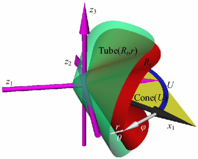
Figure 6: As for Figure 5, but for the likelihood ratio test statistic $T_{\rm LR}$ at a threshold $t=3$, cut at $||z||\leq 1$; $\phi=\arccos(t/\sqrt{n+t^{2}})=\pi/6$.

Theorem 3.

If $\text{Cone}(U)$ is convex then the EC density of the likelihood ratio cone random field $T_{\rm LR}$ is

$$\rho_{d}^{\rm LR}(t)=\sum_{j=1}^{n}p_{j}(U)\rho_{d}^{\rm F}\left(\frac{t^{2}}{j}\frac{n-j}{n};j,n-j\right)$$

The EC densities are valid for $d<n$.

Remark: As for $T_{\rm IN}$, the representation (9) represents $T_{\rm LR}$ as a patchwork mixture of $\sqrt{jn/(n-j)\cdot F_{j,n-j}}$ random fields with weights $p_{j}(U)$. See Remark 2 after Theorem 1 for why Theorem 3 should not be surprising. For the case of non-convex $\text{Cone}(U)$, see Remark 1 after Theorem 1.

Proof: It is easier to transform to the equivalent correlation coefficient

$$C=\frac{T_{\rm LR}}{\sqrt{n+T_{\rm LR}^{2}}}=\frac{\bar{\chi}}{||Z||}=\max_{u\in U}\frac{u^{\prime}Z}{||Z||}.$$

Then the rejection region $C\geq c$ is simply a cone centered at the origin that intersects the unit sphere in a tube of geodesic radius $\phi=\arccos c=\arccos(t/\sqrt{n+t^{2}})$ about $U$:

$$R_{t}=\left\{z:\arccos\left(\max_{u\in U}\frac{u^{\prime}z}{||z||}\right)\leq\phi\right\}.$$

When $\text{Cone}(U)$ is convex there is an exact expression for the probability content of a tube about a subset of the sphere, similar to (8) (Lin and Lindsay, 1997; Takemura and Kuriki, 1997):

$${\mathbb{P}}\left(\frac{\bar{\chi}}{||Z||}\geq c\right)={\mathbb{P}}(Z\in R_{t})=\sum_{j=1}^{n}p_{j}(U){\mathbb{P}}\left(\arccos(\sqrt{B_{j}})\leq\phi\right)$$

where $B_{j}$ is a Beta random variable with parameters $j/2,(n-j)/2$ (with $B_{n}=1$ with probability one). The restriction of $\text{Cone}(U)$ to a convex set is not necessary, as it was for $\bar{\chi}$ - the only requirement is that $t$ must be sufficiently large (i.e. $\phi$ must be sufficiently small) so that the tube does not self-intersect. This phenomenon is similar to what occurs when establishing the accuracy of (11) for non-convex regions $\text{Cone}(U)$. If $\text{Cone}(U)$ is convex then $t\geq 0$ suffices.

The next step is to put a tube about the rejection region $R_{t}$. Provided $r$ is sufficiently small, a (Euclidean) tube of radius $r$ about $R_{t}$ intersects the sphere of radius $||z||$ in a spherical tube of geodesic radius $\theta=\arcsin(r/||z||)$ about $R_{t}$. For fixed $||z||$ sufficiently large, $R_{t}$ is already a spherical tube about $||z||U$, so the (Euclidean) tube about $R_{t}$ is a spherical tube about $||z||U$ of geodesic radius $\phi+\theta$:

$${\rm Tube}(R_{t},r)=\left\{z:\arccos\left(\max_{u\in U}\frac{u^{\prime}z}{||z||}\right)\leq\phi+\theta\right\}.$$

The part of the tube near the origin with small $||z||$ may contain a “wedge” of the ball of radius $r$ (see Figure 5(a)) that is the only part of the whole tube that contributes to the coefficient of $r^{n}$. As pointed out in Section 2.4, $T_{\rm LR}$ is only defined for $d\leq D<n$ so we can ignore this. It therefore follows that it is sufficient for us to work with

$${\mathbb{P}}\left(Z\in{\rm Tube}(R_{t},r)\right)=\sum_{j=1}^{n}p_{j}(U){\mathbb{P}}\left(\arccos(\sqrt{B_{j}})\leq\phi+\Theta\right)+O(r^{n}),$$ (21)

where $\Theta=\arcsin(r/||Z||)$ is independent of $B_{j}$. The inequality in (21) is

$$\arccos(\sqrt{B_{j}})-\phi\leq\Theta\Longleftrightarrow\sqrt{1-B_{j}}c-\sqrt{B_{j}}\sqrt{1-c^{2}}\leq\frac{r}{||Z||},$$

so that

$${\mathbb{P}}\left(\arccos(\sqrt{B_{j}})\leq\phi+\Theta\right)={\mathbb{P}}\left(\chi_{j}\geq\chi_{n-j}\sqrt{\frac{t^{2}}{n}}-r\sqrt{1+\frac{t^{2}}{n}}\right),$$

where $\chi_{j}$ and $\chi_{n-j}$ are the square roots of independent $\chi^{2}$ random variables with degrees of freedom indicated by their subscripts. Putting everything together, the EC density that we seek is the coefficient of $r^{d}(2\pi)^{d/2}/d!$ in

$${\mathbb{P}}\left(Z\in{\rm Tube}(R_{t},r)\right)=\sum_{j=1}^{n}p_{j}(U){\mathbb{P}}\left(\chi_{j}\geq\chi_{n-j}\sqrt{\frac{t^{2}}{n}}-r\sqrt{1+\frac{t^{2}}{n}}\right)+O(r^{n}).$$

Since this expression is linear in the tube probabilities, we can differentiate immediately to arrive at the result we are looking for. $\Box$

4 Application

Friman et al. (2003) and Calhoun et al. (2004) proposed the cone and one-sided F-statistics for the detection of functional magnetic resonance (fMRI) activation in the presence of unknown delay in the hemodynamic response. We illustrate our methods with a re-analysis of the fMRI data from study an pain perception that was used by Worsley and Taylor (2006). The data, fully described in Worsley et al. (2002), consists of a time series of 3D fMRI images $Z(s,\tau)$ at point $s\in\mathbb{R}^{3}$ in the brain at time $\tau$. The subject received an alternating 9 second painful then neutral heat stimulus to the right calf, interspersed with 9 seconds of rest, repeated 10 times. The mean of the fMRI data is modeled as the indicator for each stimulus ($g(\tau)=1$ if on, 0 if not) convolved with a known hemodynamic response function (hrf) $h_{0}(\tau)$ that delays and disperses the stimulus by about 5.5 seconds (see Figure 7). Taking $g(\tau)$ as just the painful heat stimulus, we add this to a linear model for the fMRI data:

$$Z(s,\tau)=(h_{0}\star g)(\tau)\beta(s)+\sigma(s)\epsilon(s,\tau),$$

where $\epsilon(s,\tau)\sim{\rm N}(0,1)$. Our main interest is to detect regions of the brain that are ‘activated’ by the hot stimulus, that is, points $s$ where $\beta(s)>0$.

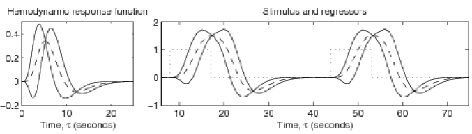
Figure 7: The hemodynamic response function $h_{0}$ (left, dashed line) and the two extremes $h_{0}\pm 2\dot{h}_{0}$ (left, solid lines) convolved with the on-off painful heat stimulus $g$ (right, dotted line) to give the “middle” of the cone $u$ (right, dashed line) and the two cone edges, the regressors $x_{1,2}=(h_{0}\pm 2\dot{h}_{0})\star g$ (right, solid lines). The on-off stimulus is repeated ten times, from 0 to 360 seconds.

There is often some doubt about the 5.5 second delay of the hrf, so to allow for unknown delay, we shift $h_{0}(\tau)$ by an amount $\delta(s)$ and add $\delta(s)$ as a parameter to the hrf. To keep the linear model, we then approximate the shifted hrf by a Taylor series expansion in $\delta(s)$ (Friston et al., 1998):

$$h(\tau;\delta(s))=h_{0}(\tau-\delta(s))\approx h_{0}(\tau)-\delta(s)\dot{h}_{0}(\tau).$$

The convolution of $h(\tau;\delta(s))$ with the stimulus $g(\tau)$ is then roughly equivalent to adding the convolution of $-\dot{h}_{0}(\tau)$ with the stimulus as an extra regressor to give the linear model:

$$Z(s,\tau)=(h_{0}\star g)(\tau)\beta(s)-(\dot{h}_{0}\star g)(\tau)\beta(s)\delta(s)+\sigma(s)\epsilon(s,\tau).$$

However the key ingredient in the model is that there is some structure to the coefficients dictated by the physical nature of the regressors. It is strongly suspected that $\beta(s)>0$ and the shift is restricted to a range of known plausible values $\delta(s)\in[\Delta_{1},\Delta_{2}]$. In our example, we take $[\Delta_{1},\Delta_{2}]=[-2,2]$ seconds. It is easy to see that the restrictions specify a non-negative-coefficient regression model

$$Z(s,\tau)=x_{1}(\tau)\beta_{1}(s)+x_{2}(\tau)\beta_{2}(s)+\sigma(s)\epsilon_{i}(s,\tau),\ \ \ \ \ \beta_{1}(s)\geq 0,\beta_{2}(s)\geq 0,$$

with regressors $x_{j}=(h-\Delta_{j}\dot{h})\star g$, $j=1,2$, illustrated in Figure 7. The model is sampled at $n$ equal intervals over time and suppose for simplicity that the resulting observations are independent. Replacing dependence on $\tau$ by vectors in $\mathbb{R}^{n}$, the linear model is the same as (3) with $m=2$:

$$Z(s)=x_{1}\beta_{1}(s)+x_{2}\beta_{2}(s)+\sigma(s)\epsilon(s),\ \ \ \ \ \beta_{1}(s)\geq 0,\beta_{2}(s)\geq 0,$$ (22)

where $\epsilon(s)$ is a vector of $n$ iid stationary Gaussian random fields. This model (22) is of course a 2D ($k=2$) cone alternative with cone angle

$$\alpha=\arccos\left(x_{1}^{\prime}x_{2}/(||x_{1}||\cdot||x_{2}||)\right).$$ (23)

The cone intrinsic volumes are ${\cal L}_{0,1}(U)=1,\alpha$, and the $\bar{\chi}$ weights are $p_{1,2}(U)=1/2,\alpha/(2\pi)$. The “middle” of the cone is $u=(x_{1}+x_{2})/2$, appropriately normalized, which of course corresponds to the unshifted model with $\delta=0$.

In practice our observations were temporally correlated and we added regressors to allow for the neutral heat stimulus and a cubic polynomial in the scan time to allow for drift, leaving $n=112$ effectively independent observations sampled every 3 seconds. The resulting $\alpha$, found by whitening the regressors and removing the effect of the added nuisance regressors before calculating (23), now depends on $s$ since the temporal correlation depends on $s$. However $\alpha$ was remarkably constant across the brain, averaging at $\alpha=1.06\pm 0.03$ radians or $60.9\pm 1.7^{\circ}$, so we take it as fixed at its mean value.

The search region $S$ is the entire brain. The error random fields $\epsilon_{i}(s)$ are not isotropic, so we must use Lipschitz-Killing curvatures of $S$ instead of intrinsic volumes. The highest order term with $d=D$ makes the largest contribution to the P-value approximation (11), and fortunately there is a very simple unbiased estimator for ${\cal L}_{D}(S)$ (Worsley et al., 1999; Taylor and Worsley, 2007). At a particular voxel, let $E$ be the $n\times 1$ vector of least-squares residuals from (22), and let $N=E/||E||$. Let $Q$ be the $n\times D$ matrix of their spatial nearest neighbor differences, that is, column $d$ of $Q$ is $N(s_{2})-N(s_{1})$ where $s_{1},s_{2}$ are neighbors on lattice axis $d$. Then the estimator of ${\cal L}_{D}(S)$ is

$$\widehat{\cal L}_{D}(S)=\sum{\rm det}(Q^{\prime}Q)^{1/2},$$

where summation is taken over all voxels inside $S$ (Worsley et al., 1999; Taylor and Worsley, 2007). The result is $\widehat{\cal L}_{3}(S)=8086$, which is of course unitless. The lower order Lipschitz-Killing curvatures are much more difficult to estimate, but they can be very accurately approximated by those of a ball with the same volume, that is with radius $r=12.5$, to give $\widehat{\cal L}_{0,1,2}(S)=1,4\pi r,2\pi r^{2}$.

We are now ready to use (11) to get approximate P-values for the maximum of our test statistic random fields. Since the degrees of freedom $\nu=110$ is so large, the two cone statistics were almost identical, so we only show results for the independently normalized cone statistic. The $P=0.05$ thresholds are shown in Table 1. Note that the values of the statistics are increasing since the cone is getting larger, but of course the $P=0.05$ thresholds are increasing as well to compensate for this. The net result is that the volume of detected activation due to the painful heat stimulus remains roughly the same. Interestingly, it is the cone statistic with delays in the range $[-2,2]$ seconds that detects the most activation. This activation is shown in Figure 8 (left primary somatosensory area and left and right thalamus).

The last question is which test is the most powerful. Worsley and Taylor (2006) gives a power comparison of the four tests that shows that if the true delay is in the range $[-1,1]$ seconds then the usual T-statistic $T_{1}$ is the most powerful, but outside this range, the cone statistic is the most powerful.

Test statistic	$P=0.05$ threshold	Detected volume (cc)
(a) T-statistic, $T_{1}$	5.15	4.0
(b) Cone statistic, $T_{\rm LR}\approx T_{\rm IN}$	5.44	4.3
(c) One-sided F-statistic, $\sqrt{2F_{+}}$	5.63	3.8
(d) F-statistic, $\sqrt{2F}$	5.80	2.9

Table 1: Test statistics, $P=0.05$ thresholds, and volume of detected activation for the application in Figure 8, in order of increasing threshold. The cone statistic detects the most activation.

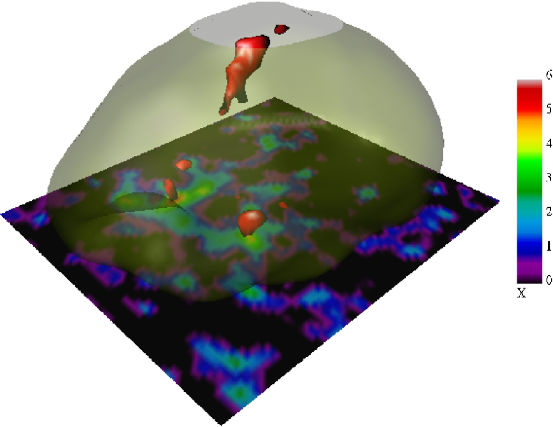
(a) (b)

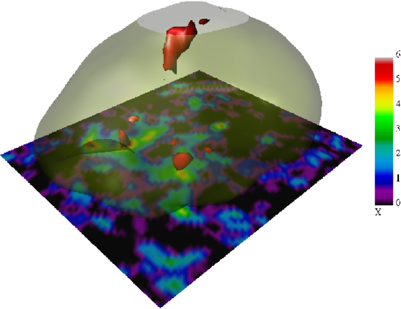
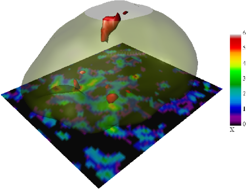
(c) (d)

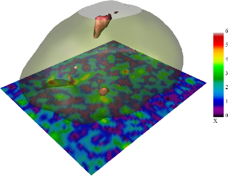
Figure 8: Detecting activation in fMRI data. Each image shows the search region (the brain, left front facing viewer) and a slice of the test statistic (color coded) thresholded at $P=0.05$ (red-pink blobs - see Table 1). The test statistics, in order of increasing threshold, are (a) the T-statistic $T_{1}$; (b) the cone statistic $T_{\rm IN}$ (indistinguishable from $T_{\rm LR}$ in this case); (c) the square root of twice the one-sided F-statistic $\sqrt{2F_{+}}$; (d) the square root of twice the F-statistic $\sqrt{2F}$.

Appendix A Intrinsic volume

The $d$-dimensional intrinsic volume of a set $S$ is a generalization of its volume to lower dimensional measures. The $D$-dimensional intrinsic volume of $S\subset\mathbb{R}^{D}$ is its usual volume or Lebesgue measure, the $(D-1)$-dimensional intrinsic volume of $S$ is half its surface area, and the $0$-dimensional intrinsic volume is the Euler characteristic of $S$. The simplest definition is implicit, identifying the intrinsic volumes as coefficients in a certain polynomial. This definition comes from the Steiner-Weyl volume of tubes formula which states that if $S$ has no concave ‘corners’, then for $r$ small enough

$$|{\rm Tube}(S,r)|=\sum_{d=0}^{D}\omega_{D-d}r^{D-d}{\cal L}_{d}(S)$$ (24)

where $|\cdot|$ denotes Lebesgue measure and $\omega_{d}=\pi^{d/2}/\Gamma(d/2+1)$ is the Lebesgue measure of the unit ball in $\mathbb{R}^{d}$.

If $S$ is bounded by a smooth hypersurface, so that there is a unique normal vector at each point on the boundary, then a more direct definition is as follows. Let $C(s)$ be the $(D-1)\times(D-1)$ inside curvature matrix at $s\in\partial S$, the boundary of $S$. To compute the intrinsic volumes, we need the det-traces of a square matrix: for a $d\times d$ symmetric matrix $A$, let ${\rm detr}_{j}(A)$ denote the sum of the determinants of all $j\times j$ principal minors of $A$, so that ${\rm detr}_{d}(A)=\det(A)$, ${\rm detr}_{1}(A)={\rm tr}(A)$, and we define ${\rm detr}_{0}(A)=1$. Let $a_{d}=2\pi^{d/2}/\Gamma(d/2)$ be the $(d-1)$-dimensional Hausdorff (surface) measure of the unit $(d-1)$-sphere in $\mathbb{R}^{d}$. For $d=0,\dots,D-1$ the $d$-dimensional intrinsic volume of $S$ is

$${\cal L}_{d}(S)={{1}\over{a_{D-d}}}\int_{\partial S}{\rm detr}_{D-1-d}\{C(s)\}ds,$$

and ${\cal L}_{D}(S)=|S|$, the Lebesgue measure of $S$. Note that ${\cal L}_{0}(S)=\varphi(S)$ by the Gauss-Bonnet Theorem, and ${\cal L}_{D-1}(S)$ is half the surface area of $S$.

For the unit $(k-1)$-sphere, $C=\pm I_{(k-1)\times(k-1)}$ on the outside/inside of $O^{k-1}$, so that

$${\cal L}_{d}(O^{k-1})=2{k-1\choose d}\frac{a_{k}}{a_{k-d}}=\frac{2^{d+1}\pi^{d/2}\Gamma\left(\frac{k+1}{2}\right)}{d!\Gamma\left(\frac{k+1-d}{2}\right)}$$ (25)

if $k-1-d$ is even, and zero otherwise, $d=0,\dots,k-1$.

References

- Adler (1981) Adler, R. J. (1981). The Geometry of Random Fields. John Wiley & Sons, Chichester.
- Adler (2000) Adler, R. J. (2000). On excursion sets, tube formulae, and maxima of random fields. Annals of Applied Probability, 10 1–74.
- Adler and Taylor (2007) Adler, R. J. and Taylor, J. E. (2007). Random fields and their geometry. Birkhäuser, Boston.
- Becker et al. (2009) Becker, S., Bobin, J. and Candès, E. J. (2009). NESTA: a fast and accurate first-order method for sparse recovery. SIAM J. on Imaging Sciences, 4 1–39.
- Birnbaum (1954) Birnbaum, A. (1954). Combining independent tests of significance. Journal of the American Statistical Society, 49 559–574.
- Calhoun et al. (2004) Calhoun, V., Stevens, M., Pearlson, G. and Kiehl, K. (2004). fMRI analysis with the general linear model: removal of latency-induced amplitude bias by incorporation of hemodynamic derivative terms. NeuroImage, 22 252–257.
- Cao and Worsley (1999a) Cao, J. and Worsley, K. (1999a). The geometry of correlation fields with an application to functional connectivity of the brain. Annals of Applied Probability, 9 1021–1057.
- Cao and Worsley (1999b) Cao, J. and Worsley, K. J. (1999b). The detection of local shape changes via the geometry of Hotelling’s fields. Annals of Statistics, 27 925–942.
- Carbonell and Worsley (2007) Carbonell, F. and Worsley, K. (2007). The geometry of the Wilks’s random field. Annals of the institute of Statistical Mathematics. Submitted.
- Cohen and Sackrowitz (1993) Cohen, A. and Sackrowitz, H. B. (1993). Inadmissibility of studentized tests for normal order restricted models. Annals of Statistics, 21 746–752.
- Friedman et al. (2007) Friedman, J. H., Hastie, T., Hofling, H. and Tibshirani, R. (2007). Pathwise coordinate optimization. Annals of Applied Statistics, 1 302–332.
- Friman et al. (2003) Friman, O., Borga, M., Lundberg, P. and Knutsson, H. (2003). Adaptive analysis of fMRI data. NeuroImage, 19 837–845.
- Friston et al. (1998) Friston, K., Fletcher, P., Josephs, O., Holmes, A., Rugg, M. and Turner, R. (1998). Event-related fMRI: Characterising differential responses. NeuroImage, 7 30–40.
- Friston et al. (1995) Friston, K. J., Holmes, A. P., Worsley, K. J., Poline, J. P., Fritn, C. D. and Frackowiak, R. S. (1995). Statistical parametric maps in functional imaging a general linear approach. Human Brain Mapping, 2 189–210.
- Johansen and Johnstone (1990) Johansen, S. and Johnstone, I. (1990). Hotelling’s theorem on the volume of tubes: some illustrations in simultaneous inference and data analysis. Annals of Statistics, 18 652–684.
- Johnstone and Siegmund (1989) Johnstone, I. and Siegmund, D. (1989). On hotelling’s formula for the volume of tubes and naiman’s inequality. The Annals of Statistics, 17 184–194.
- Knowles and Siegmund (1989) Knowles, M. and Siegmund, D. (1989). On Hotelling’s approach to testing for a nonlinear parameter in a regression. International Statistical Review, 57 205–220.
- Lawson and Hanson (1995) Lawson, C. L. and Hanson, R. J. (1995). Solving Least Squares Problems. Society for Industrial and Applied Mathematics, Philadelphia.
- Lin and Lindsay (1997) Lin, Y. and Lindsay, B. G. (1997). Projections on cones, chi-bar squared distributions, and Weyl’s formula. Statistics & Probability Letters, 32 367–376.
- Nardi et al. (2008) Nardi, Y., Siegmund, D. O. and Yakir, B. (2008). The distribution of maxima of approximately Gaussian random fields. Annals of Statistics, 36.
- Perlman and Wu (1999) Perlman, M. D. and Wu, L. (1999). The Emperor’s new tests. Statistical Science, 14 355–381.
- Pilla (2006) Pilla, R. S. (2006). Inference under convex cone alternatives for correlated data. E-print. ArXiv:math/0506522v3.
- Polzehl and Tabelow (2006) Polzehl, J. and Tabelow, K. (2006). Analysing fMRI experiments with the fmri package in R. Version 1.0 - A users guide. Weierstrass Institute for Applied Analysis and Stochastics Technical Report, 10.
- Robertson et al. (1988) Robertson, T., Wright, F. T. and Dykstra, R. L. (1988). Order Restricted Statistical Inference. Wiley, New York.
- Shafie et al. (2003) Shafie, K., Sigal, B., Siegmund, D. O. and Worsley, K. J. (2003). Rotation space random fields with an application to fMRI data. Annals of Statistics, 31 1732–1771.
- Siegmund and Worsley (1995) Siegmund, D. O. and Worsley, K. J. (1995). Testing for a signal with unknown location and scale in a stationary Gaussian random field. Annals of Statistics, 23 608–639.
- Sun (1993) Sun, J. (1993). Tail probabilities of the maxima of Gaussian random fields. Annals of Probability, 21 34–71.
- Sun and Loader (1994) Sun, J. and Loader, C. R. (1994). Simultaneous confidence bands for linear regression and smoothing. Annals of Statistics, 22 1328–1345.
- Sun et al. (2000) Sun, J., Loader, C. R. and McCormick, W. P. (2000). Confidence bands in generalized linear models. Annals of Statistics, 28 429–460.
- Takemura and Kuriki (1997) Takemura, A. and Kuriki, S. (1997). Weights of distribution for smooth or piecewise smooth cone alternatives. Annals of Statistics, 25 2368–2387.
- Takemura and Kuriki (2002) Takemura, A. and Kuriki, S. (2002). On the equivalence of the tube and Euler characteristic methods for the distribution of the maximum of Gaussian fields over piecewise smooth domains. Annals of Applied Probability, 12 768–796.
- Taylor (2006) Taylor, J. E. (2006). A Gaussian kinematic formula. Annals of Probability, 34 122–158.
- Taylor and Adler (2003) Taylor, J. E. and Adler, R. J. (2003). Euler characteristics for Gaussian fields on manifolds. Annals of Probability, 31 533–563.
- Taylor et al. (2005) Taylor, J. E., Takemura, A. and Adler, R. J. (2005). Validity of the expected Euler characteristic heuristic. Annals of Probability, 33 1362–1396.
- Taylor and Vadlamani (2011) Taylor, J. E. and Vadlamani, S. (2011). Random fields and the geometry of Wiener space. Annals of Probability. To appear., URL http://arxiv.org/abs/1105.3839.
- Taylor and Worsley (2007) Taylor, J. E. and Worsley, K. J. (2007). Detecting sparse signals in random fields, with an application to brain mapping. Journal of the American Statistical Association, 102 913–928.
- Taylor and Worsley (2008) Taylor, J. E. and Worsley, K. J. (2008). Random fields of multivariate test statistics, with applications to shape analysis. The Annals of Statistics, 36 1–27.
- Worsley et al. (1999) Worsley, K., Andermann, M., Koulis, T., MacDonald, D. and Evans, A. (1999). Detecting changes in nonisotropic images. Human Brain Mapping, 8 98–101.
- Worsley et al. (2002) Worsley, K., Liao, C., Aston, J., Petre, V., Duncan, G., Morales, F. and Evans, A. (2002). A general statistical analysis for fMRI data. NeuroImage, 15 1–15.
- Worsley and Taylor (2006) Worsley, K. and Taylor, J. (2006). Detecting fMRI activation allowing for unknown latency of the hemodynamic response. NeuroImage, 29 649–654.
- Worsley (1994) Worsley, K. J. (1994). Local maxima and the expected Euler characteristic of excursion sets of and fields. Advances in Applied Probability, 26 13–42.
- Worsley (1995a) Worsley, K. J. (1995a). Boundary corrections for the expected Euler characteristic of excursion sets of random fields, with an application to astrophysics. Advances in Applied Probability, 27 943–959.
- Worsley (1995b) Worsley, K. J. (1995b). Estimating the number of peaks in a random field using the hadwiger characteristic of excursion sets, with applications to medical images. The Annals of Statistics, 23 640–669.
- Worsley (2001) Worsley, K. J. (2001). Testing for signals with unknown location and scale in a random field, with an application to fMRI. Advances in Applied Probability, 33 773–793.
- Worsley et al. (1996) Worsley, K. J., Marrett, S., Neelin, P., Vandal, A. C., Friston, K. J. and Evans, A. C. (1996). A unified statistical approach for determining significant signals in images of cerebral activation. Human Brain Mapping, 4 58–73.