Tracking Tetrahymena Pyriformis Cells using Decision Trees

Abstract

Matching cells over time has long been the most difficult step in cell tracking. In this paper, we approach this problem by recasting it as a classification problem. We construct a feature set for each cell, and compute a feature difference vector between a cell in the current frame and a cell in a previous frame. Then we determine whether the two cells represent the same cell over time by training decision trees as our binary classifiers. With the output of decision trees, we are able to formulate an assignment problem for our cell association task and solve it using a modified version of the Hungarian algorithm.

1 Introduction

Researchers have been creating artificial magnetotactic Tetrahymena pyriformis (T. pyriformis) cells by the internalization of iron oxide nano particles, and controlling them with a time-varying external magnetic field [2, 5]. To perform the multi-cell control task, it is necessary to track the real-time position of each cell and use it as the feedback for the control system. However, this problem is very difficult because: the T. pyriformis cells are moving fast in the field of view; several cells may overlap and occlude each other; the appearances of different cells can be similar; and the same cell may change in appearance over time [4].

Decision tree was proposed as a powerful machine learning technique, which can be used for both classification and regression, and has been successfully applied on practical systems such as the Kinect gaming platform [6]. Since the decision tree can take very complicated features as its input and at the same time, once a decision tree is trained, the decision procedure can be very fast, it is ideal for real-time classification. We use decision trees as a classifier to determine whether regions segmented in neighboring and non-neighboring frames represent the same T. pyriformis cell.

2 Background Subtraction

To extract the foreground regions of cells, we first perform a background subtraction at each frame. There are a number of well-known background subtraction algorithms such as adaptive Gaussian mixture models. Since the background in our video is simple and consistent over time, we simply apply a median filter on the time dimension for the first 20 frames to obtain the background image. At each frame, we subtract the background image from the current frame and take the absolute value to obtain a difference image. Then we apply thresholding, fill the morphological holes, and extract the connected regions as candidate T. pyriformis cells.

3 Feature Extraction

After the region of each cell is segmented, we extract features for each cell according to their shapes, gray-level intensities, and the combination of both. Examples of the T. pyriformis cell appearance in our video are shown in Figure 1 (pixel spacing = $2.32\text{/}2.32\text{\,}\mathrm{\SIUnitSymbolMicro m}$). Assume a cell $C$ in one frame consists of $N$ pixels $I(\textbf{x}_{i})$, where $i=1,2,\dots,N$, and $\textbf{x}_{i}=(x_{i},y_{i})$ are the coordinates of the $i$th pixel of $C$. We can define some useful features for this cell, as follows.

Spatial Features

The cell’s area $N$ and centroid $\textbf{x}_{c}=(x_{c},y_{c})$, where $x_{c}=\overline{x_{i}}$ and $y_{c}=\overline{y_{i}}$, are the most basic features. Another useful spatial feature is the $n$th order normalized inertia [1], which measures the circularity of the shape, and is defined as

$$J_{n}(C)=\dfrac{\sum\limits_{i=1}^{N}||\textbf{x}_{i}-\textbf{x}_{c}||^{n}}{N^{1+n/2}}.$$ (1)

Histogram Features

Using only pixel intensities without spatial positions, we can compute several histogram features. First we have the mean and the standard deviation:

$$\mu(C) = \dfrac{1}{N}\sum\limits_{i=1}^{N}I(\textbf{x}_{i}),$$ (2)

$$\sigma(C) = \dfrac{1}{N}\sqrt{\sum\limits_{i=1}^{N}\left(I(\textbf{x}_{i})-\mu(C)\right)^{2}}.$$ (3)

Then we have the standard moments such as the skewness $\gamma(C)$ and the kurtosis $\beta(C)$:

$$\gamma(C) = E\left[\left(\dfrac{I(\textbf{x}_{i})-\mu(C)}{\sigma(C)}\right)^{3}\right],$$ (4)

$$\beta(C) = E\left[\left(\dfrac{I(\textbf{x}_{i})-\mu(C)}{\sigma(C)}\right)^{4}\right],$$ (5)

where $E[\cdot]$ denotes expectation. We also use the $n$th order root of the $n$th order central moment $M_{n}(C)$:

$$M_{n}(C)=\sqrt[n]{E\left[\left(I(\textbf{x}_{i})-\mu(C)\right)^{n}\right]}.$$ (6)

Composite Features

Finally we can compute some features that use both spatial information and pixel intensities at the same time to capture the spatial distribution of pixel intensities. We first define the polynomial distribution feature $P_{n}(C)$:

$$P_{n}(C)=\dfrac{1}{N^{1+n/2}}\sum\limits_{i=1}^{N}||\textbf{x}_{i}-\textbf{x}_{c}||^{n}\cdot I(\textbf{x}_{i}).$$ (7)

Then we define the Gaussian distribution feature $G_{n}(C)$:

$$G_{n}(C)=\dfrac{1}{N}\sum\limits_{i=1}^{N}\exp\left(-\dfrac{||\textbf{x}_{i}-\textbf{x}_{c}||^{2}}{2n^{2}}\right)\cdot I(\textbf{x}_{i}).$$ (8)

These composite features can be viewed as weighted means of pixel intensities. For example, $P_{n}(C)$ gives larger weights to pixels far away from the center while $G_{n}(C)$ gives larger weights to pixels near the center.

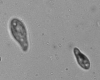
(a)

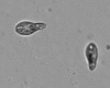
(b)

Figure 1: Examples of the T. pyriformis cell appearance.

4 Decision Trees

To use decision trees for the cell association problem, we first need to map the cell association problem to a classification problem. For each cell $L$ in a previous frame and each cell $C$ in the current frame, we need to know whether they are the same cell. Thus the classification problem is to develop a binary classifier $f$ such that $f(C,L)=1$ if $C$ and $L$ are the same cell, and $f(C,L)=0$ if they are not.

4.1 Feature Difference Vector

To simplify the input to the classifier, we define a 23-dimensional feature difference vector $\textbf{v}(C,L)=(v_{1},v_{2},\dots,v_{23})$ for $C$ and $L$. Each entry of this feature difference vector reflects the difference of the two cells in some aspect. $v_{1}$ is the distance between the center of $C$ and the predicted center of $L$ in the current frame. A simple constant velocity assumption is used for the prediction. For example, suppose the current frame is the $k$th frame and the center of $C$ is $\textbf{x}_{c}(C)$, the center of $L$ at the $(k-1)$th frame was $\textbf{x}_{c}(L)$ and at the $(k-2)$th frame was $\textbf{x}^{\prime}_{c}(L)$. Then the predicted center of $L$ at the current frame is $\textbf{x}_{p}(L)=2\textbf{x}_{c}(L)-\textbf{x}^{\prime}_{c}(L)$, and $v_{1}$ is defined as

$$v_{1}=||\textbf{x}_{c}(C)-\textbf{x}_{p}(L)||.$$ (9)

$v_{2}$ is defined as the distance between the centers of the two cells:

$$v_{2}=||\textbf{x}_{c}(C)-\textbf{x}_{c}(L)||.$$ (10)

Each of the other 21 entries of $\textbf{v}(C,L)$ is defined as the absolute value of the difference of some feature of $C$ and $L$. For example, let $N(C)$ and $N(L)$ be the areas of $C$ and $L$, respectively. Then we have

$$v_{3} = |N(C)-N(L)|,$$ (11)

$$v_{4} = |\mu(C)-\mu(L)|.$$ (12)

Similarly, $v_{5}$ to $v_{7}$ are defined using Equations (3) to (5) respectively; $v_{8}$ to $v_{11}$ are defined using (6) for $n=3,4,5,6$; $v_{12}$ to $v_{15}$ are defined using (1) for $n=1,2,3,0.5$; $v_{16}$ to $v_{19}$ are defined using (7) for $n=1,2,3,0.5$; and $v_{20}$ to $v_{23}$ are defined using (8) for $n=2,4,6,8$. With these definitions, our classifier $f$ can be viewed as a mapping from the 23-dimensional space to the $\{0,1\}$ set. Thus we denote it as $f(\textbf{v}(C,L))$.

4.2 Training a Decision Tree

As shown in Figure 2, a decision tree $T$ consists of leaf nodes and split (non-leaf) nodes. Each split node consists of a threshold $\tau$ and an indicator $k$ for a feature $v_{k}$, where $k=1,2,\dots,23$. To classify the feature difference vector v, one starts from the root and repeatedly compares its $k$th entry $v_{k}$ with the threshold $\tau$ to decide whether to branch to the left sub-tree (if $v_{k}\leq\tau$) or right sub-tree (if $v_{k}>\tau$). The leaf node is a quantity $P_{T}(\textbf{v})$ indicating the probability of $f(\textbf{v}(C,L))=1$.

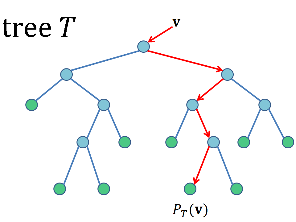
Figure 2: Decision tree example. A decision tree $T$ consists of split nodes (blue) and leaf nodes (green). The red arrows show the branching path for an input v.

Since it is easy for a human to distinguish whether two regions in different frames represent the same cell, we can manually assign labels $\{y\}$ to cell pairs from neighboring frames in training videos and associate these labels with extracted feature difference vectors $\{\textbf{v}\}$. In this way we build our training data set $D=\{(\textbf{v},y)\}$, where $y=f(\textbf{v})$.

The training process follows a maximal entropy reduction procedure [6]:

1. Beginning from the root, consider a large set of splitting candidates $(k,\tau)$ which covers all possible $k$ and provides sufficiently delicate subdivisions for each $v_{k}$.

2. For each candidate $(k,\tau)$, we partition the training set $D=\{(\textbf{v},y)\}$ into two subsets:

   $$D_{l}(k,\tau) = \{(\textbf{v},y)|v_{k}\leq\tau\},$$ (13)

   $$D_{r}(k,\tau) = D\setminus D_{l}(k,\tau).$$ (14)

3. Find the candidate $(k,\tau)$ that maximizes the entropy reduction $G(k,\tau)$:

   $$(k^{*},\tau^{*})=\underset{(k,\tau)}{\operatorname{argmax}}\;G(k,\tau),$$ (15)

   $$G(k,\tau) = H(D)-\dfrac{|D_{l}(k,\tau)|}{|D|}H(D_{l}(k,\tau))$$ (16)

   $$-\dfrac{|D_{r}(k,\tau)|}{|D|}H(D_{r}(k,\tau)),$$

   where $H(\cdot)$ denotes the Shannon entropy and $|\cdot|$ denotes the cardinality of a set.

4. Use $(k^{*},\tau^{*})$ as the feature indicator and threshold at the current split node, and repeat the above steps for the left sub-tree with $D_{l}(k^{*},\tau^{*})$ and right sub-tree with $D_{r}(k^{*},\tau^{*})$.

5. If the depth reaches the maximum, or the size (or entropy) of the partitioned subset $\widetilde{D}$ at the current node is sufficiently small, then we set this node as a leaf node, and the probability at this node is

   $$P_{T}=\dfrac{|\{(\textbf{v},y)\in\widetilde{D}|y=1\}|}{|\widetilde{D}|}.$$ (17)

In our work, a tree $T_{1}$ is trained using $D=\{{(\textbf{v},y)}\}$, and another tree $T_{2}$ is trained using $D^{\prime}=\{{(\textbf{v}^{\prime},y)}\}$, where $\textbf{v}^{\prime}=(v_{3},v_{4},\dots,v_{23})$ is the truncated feature difference vector. Since $T_{2}$ is trained without center position information, we use $T_{1}$ for cell association in neighboring frames and $T_{2}$ for cell association in non-neighboring frames.

5 Association Rules

To track cells over time, we maintain a list $\{L_{j}\}$ of cells that have appeared in previous frames. The cell association task is to determine which cell $L_{j}$ should be associated with the cell $C_{i}$ in the current frame. Each cell in the list has a status, being active, occluded, out, or new.

5.1 Association Matrix

At frame $k$, if we have $N_{1}$ cells $\{C_{i}\}$ in the current frame and $N_{2}$ cells $\{L_{j}\}$ in the list, we define an $N_{1}\times(N_{2}+2)$ association matrix $A$. Each entry of $A$ represents the confidence of associating $C_{i}$ with a cell in the list or considering it as a new cell.

If $1\leq j\leq N_{2}$ and the status of $L_{j}$ is active, new or occluded, we define

$$A_{i,j}=P_{T_{1}}(\textbf{v}(C_{i},L_{j})).$$ (18)

Let $d_{0}$ denote the maximum possible speed of a T. pyriformis cell in pixels per frame, and $d_{b}(C_{i})$ denote the distance from $C_{i}$ to the image border. A new cell or a re-appearing cell must (re-)enter the image from the image border. Thus for $1\leq j\leq N_{2}$, if the status of $L_{j}$ is out and $d_{b}(C_{i})>d_{0}$, we set $A_{i,j}=-1$; if the status of $L_{j}$ is out and $d_{b}(C_{i})\leq d_{0}$, we define

$$A_{i,j}=\alpha_{1}P_{T_{2}}(\textbf{v}^{\prime}(C_{i},L_{j})),$$ (19)

where $0<\alpha_{1}<1$ is a constant denoting the diffidence (as shown in Table 1) of associating cells in non-neighboring frames.

$A_{i,N_{2}+1}$ is the confidence of considering $C_{i}$ as a new cell that has not appeared in previous frames. If $d_{b}(C_{i})>d_{0}$, we set $A_{i,N_{2}+1}=-1$; if $d_{b}(C_{i})\leq d_{0}$, we define

$$A_{i,N_{2}+1}=\alpha_{2}\exp(-\lambda_{1}d_{b}^{2}(C_{i})),$$ (20)

where $0<\alpha_{2}<1$ and $\lambda_{1}>0$ are two constants.

To also include the case when one cell is occluded by another, we use $A_{i,N_{2}+2}$ to represent the confidence that $C_{i}$ is a region of more than one cell overlapping. Let $\{L_{j}^{\prime}\}$ be a subset of the list containing only cells that have appeared in the $(k-1)$th frame. We define

$$A_{i,N_{2}+2}=\alpha_{3}\sum\limits_{L_{j}^{\prime}}e^{-\lambda_{2}d_{p}^{2}(C_{i},L_{j}^{\prime})}-\alpha_{3}\sum\limits_{C_{j}}e^{-\lambda_{2}d_{c}^{2}(C_{i},C_{j})},$$ (21)

where $0<\alpha_{3}<1$ and $\lambda_{2}>0$ are two constants, $d_{c}(C_{i},C_{j})$ is the center distance between $C_{i}$ and $C_{j}$, and $d_{p}(C_{i},L_{j}^{\prime})$ is the distance from the center of $C_{i}$ to the predicted center of $L_{j}^{\prime}$, which is similar to (9). The right-hand side of (21) can be thought of as the predicted number of cells minus the observed number of cells near $C_{i}$.

5.2 Association List

Once the association matrix $A$ is created, we need to associate each $C_{i}$ (or each row of $A$) with a column of $A$. This problem is similar to the standard assignment problem [3], but note that: first, $A$ is generally not a square matrix; second, more than one $C_{i}$ can be considered as new or being a region of occluded cells. We define an association list $\boldsymbol{\zeta}=(\zeta_{1},\zeta_{2},\dots,\zeta_{N_{1}})$ such that $\zeta_{i}=j$ if $C_{i}$ is associated with the $j$th column of $A$. Then our problem is to find

$$\boldsymbol{\zeta}^{*}=\underset{\boldsymbol{\zeta}}{\operatorname{argmax}}\;\sum\limits_{i=1}^{N_{1}}A_{i,\zeta_{i}}$$ (22)

such that for any $1\leq j\leq N_{2}$, there is at most one $i$ that satisfies $\zeta_{i}=j$.

5.3 The Modified Hungarian Algorithm

When $N_{1}$ and $N_{2}$ are both small, the derivative assignment problem (22) can be solved using a brute-force search. But when $N_{1}$ and $N_{2}$ are large, the computational complexity of brute-force search is at least

$$O\left(\dfrac{(\max\{N_{1},N_{2}\})!}{|N_{1}-N_{2}|!}\right),$$ (23)

which is unacceptable for real-time tracking. We propose a modified version of the Hungarian algorithm [3] to obtain a suboptimal solution of (22). The computational complexity of the original Hungarian algorithm is $O((\max\{N_{1},N_{2}\})^{3})$, and our modified Hungarian algorithm can achieve a computational complexity of at most $O((\max\{N_{1},N_{2}\})^{3}\cdot\min\{N_{1},N_{2}\})$. The modified Hungarian algorithm is given below:

1. For any $1\leq i\leq N_{1}$, if the $i$th row of $A$ satisfies

   $$\underset{j}{\operatorname{argmax}}\;A_{i,j}=j^{*}>N_{2},$$ (24)

   then we associate the $i$th row with the $j^{*}$th column, and delete the $i$th row from $A$ to obtain a $N_{1}^{\prime}\times(N_{2}+2)$ submatrix $A^{\prime}$.

2. Perform the standard Hungarian algorithm on the first $N_{2}$ columns of $A^{\prime}$ to get an association list $\boldsymbol{\zeta}$.

3. For $1\leq i\leq N_{1}^{\prime}$, compute this value:

   $$\Omega(A^{\prime},i)=\max\{A^{\prime}_{i,N_{2}+1},A^{\prime}_{i,N_{2}+2}\}-A^{\prime}_{i,\zeta_{i}}.$$ (25)

   If $\max\limits_{i}\Omega(A^{\prime},i)>0$, let

   $$i^{*}=\underset{i}{\operatorname{argmax}}\;\Omega(A^{\prime},i).$$ (26)

   Then we associate the $i^{*}$th row of $A^{\prime}$ with the $(N_{2}+1)$th column if $A^{\prime}_{i^{*},N_{2}+1}>A^{\prime}_{i^{*},N_{2}+2}$ or the $(N_{2}+2)$th column if otherwise. Now we delete the $i^{*}$th row from $A^{\prime}$, update $N_{1}^{\prime}$, and repeat steps 2 to 3.

4. If $\max\limits_{i}\Omega(A^{\prime},i)\leq 0$, then the current $\boldsymbol{\zeta}$ is the final association result for the current $A^{\prime}$.

5.4 Updating the List of Cells

We update the list of cells $\{L_{j}\}$ according to the association result of each $C_{i}$:

• If $C_{i}$ is associated with a cell $L_{j}$ in the list ($1\leq\zeta_{i}\leq N_{2}$), we update the status of $L_{j}$ to active and replace all its features with the features of $C_{i}$.

• If $C_{i}$ is considered to be a new cell ($\zeta_{i}=N_{2}+1$), we simply add it to the list and set its status to new.

• If $C_{i}$ is considered to be a region of overlapping cells ($\zeta_{i}=N_{2}+2$), we search its neighbourhood within the radius $d_{0}$ for unassociated $L_{j}$’s that have appeared in the $(k-1)$th frame. Then we set the status of these $L_{j}$’s to occluded, and update only their center positions to the center position of $C_{i}$.

• For any $L_{j}$ that appeared in the $(k-1)$th frame and is still unassociated after all the above steps: if it is within the distance $d_{0}$ from the image border, we set its status to out; otherwise, we associate it with the closest unassociated $C_{i}$.

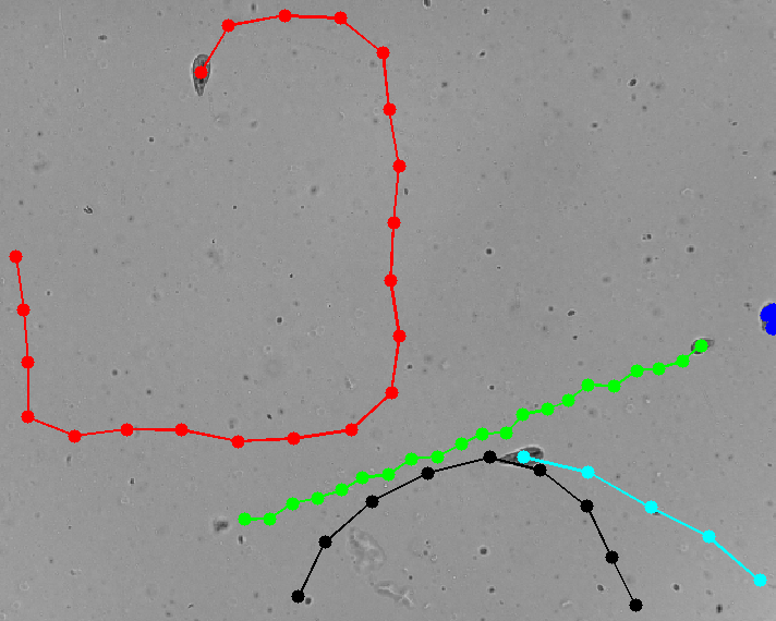
(a)

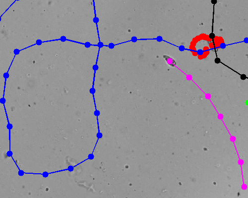
(b)

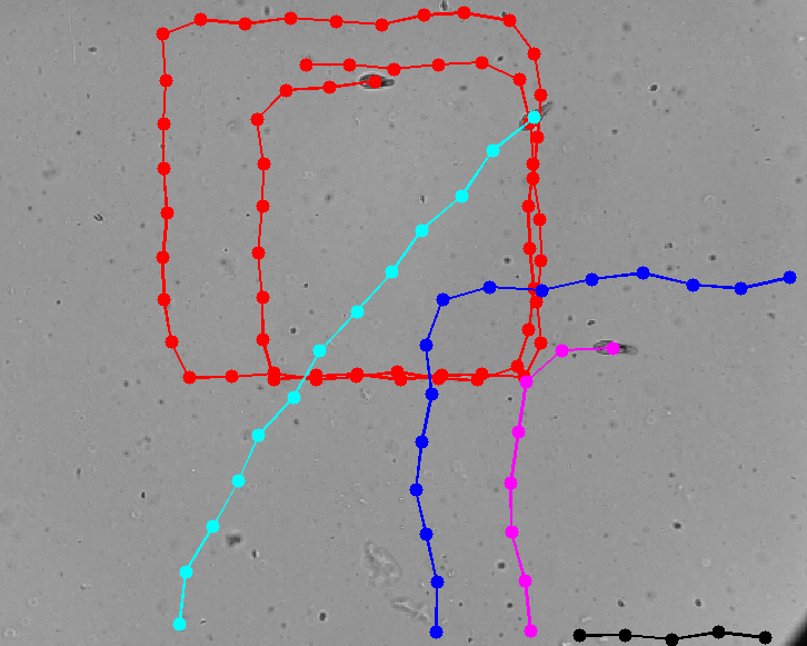
(c)

Figure 3: Resulting cell trajectories of our method on testing videos. (a) Cells getting very close. (b) Two cells occluding each other (red vs. blue, and red vs. black). (c) Many cells appearing in the frame at the same time.

6 Experiments

To build the training set, we manually label the cell regions segmented in 1000 frames from 2 videos, where each frame is an 8-bit gray-level image of size $640\times 512$, and the videos were captured at 8 frames per second [2]. The typical size of a T. pyriformis cell is between 150 and 400 pixels, and the typical speed is between 5 and 40 pixels per frame. To evaluate the performance of the decision trees $T_{1}$ and $T_{2}$, we repeat 20 independent experiments for different depth of the trees, and in each experiment we use randomly selected $70\%$ of the cell pairs as the training data, and the rest $30\%$ as the test data. The number of subdivisions of each feature is set to 1000, and the stop-splitting size of $\widetilde{D}$ is set to 20. The classifier $f$ is configured such that $f(\textbf{v})=1$ if $P_{T}(\textbf{v})>0.5$. The resulting average rates of misclassification are shown in Table 1, and all 23 entries of the feature difference vector v turn out to be useful.

Depth of Tree	Error Rate of $T_{1}$	Error Rate of $T_{2}$
5	1.48%	14.02%
6	1.46%	13.91%
7	1.69%	12.95%
8	1.37%	12.49%
9	1.54%	13.07%
10	1.55%	13.61%

Table 1: Performance of decision trees.

In our tracking experiments, we use decision trees of depth 8. The parameters $\alpha_{1}$, $\alpha_{2}$, $\alpha_{3}$, $\lambda_{1}$, $\lambda_{2}$ and $d_{0}$ are selected empirically by studying the training videos, and the tracking results are not sensitive to minor changes of these parameters. Example cell trajectories obtained by our method are shown in Figure 3. In these examples we set $\alpha_{1}=0.1$, $\alpha_{2}=0.1$, $\alpha_{3}=0.8$, $\lambda_{1}=0.00008$, $\lambda_{2}=0.00005$ and $d_{0}=70$.

7 Discussion and Future Work

This paper has shown a novel cell tracking method using decision trees as classifiers for feature difference vectors. The misclassification rates of our decision trees are very low, and the tracking results of our method are robust against cell occlusions. Future work includes evaluating this method on more complicated videos in which more cells exist in the frame and occlusions of many cells can happen. Finally we will integrate our algorithm into the real-time T. pyriformis control system.

References

- [1] A. Gersho. Asymptotically optimal block quantization. IEEE Transactions on Information Theory, 25(4):373–380, 1979.
- [2] D. H. Kim, U. K. Cheang, L. Kőhidai, D. Byun, and M. J. Kim. Artificial magnetotactic motion control of Tetrahymena pyriformis using ferromagnetic nanoparticles: A tool for fabrication of microbiorobots. Applied Physics Letters, 97(17):173702, 2010.
- [3] H. W. Kuhn. The Hungarian method for the assignment problem. Naval Research Logistic Quarterly, 2:83–97, 1955.
- [4] E. Meijering, O. Dzyubachyk, I. Smal, and W. A. van Cappellen. Tracking in cell and developmental biology. Seminars in Cell & Developmental Biology, 20(8):894–902, 2009.
- [5] Y. Ou, D. H. Kim, P. Kim, M. J. Kim, and A. A. Julius. Motion Control of Tetrahymena Pyriformis Cells with Artificial Magnetotaxis: Model Predictive Control (MPC) Approach. In IEEE International Conference on Robotics and Automation, St. Paul, USA, May 2012.
- [6] J. Shotton, A. Fitzgibbon, M. Cook, T. Sharp, M. Finocchio, R. Moore, A. Kipman, and A. Blake. Real-time human pose recognition in parts from single depth images. In Computer Vision and Pattern Recognition, June 2011.