Singlet Extension of the MSSM
for 125 GeV Higgs Mass with the Least Tuning

Abstract

In order to raise the Higgs mass to 125 GeV and relieve the fine-tuning associated with the heavy s-top mass in the minimal supersymmetric standard model (MSSM), we propose a new singlet extension of the MSSM. In this scenario, the additional Higgs mass is radiatively generated in a hidden sector, and the effect is transmitted to the Higgs through a messenger field. The Higgs mass can be efficiently increased by the parameters of the superpotential as in the extra matter scenario, but free from the constraints on extra colored matter fields by the LHC experiments. As a result, the tuning problem can be remarkably mitigated by taking low enough messenger mass ($\sim 300$ GeV) and mass parameter scales ($\sim 500$ GeV). We also discuss how to enhance the diphoton decay rate of the Higgs over the SM expectation in this framework.

I Introduction

Recently, CMS and ATLAS reported the observations of the signals, which can be interpreted as the presence of a standard model Higgs(-like) boson with the mass of 125 GeV around the five sigma confidence level CMS ; ATLAS . The news seems to be accepted as the discovery of the long-awaited Higgs particle, which is very essential in mass generations for the standard model (SM) particles. However, the theoretical issues associated with the Higgs boson, e.g. how the Higgs can naturally exist at low energies, still remain unsolved. Actually, these issues have played the role of strong motivations to study various new physics beyond the SM.

For the last three decades, the minimal supersymmetric standard model (MSSM) has maintained the status as the leading candidate beyond the SM MSSM . The MSSM provides a beautiful solution to the large hierarchy problem between the electroweak(EW) and the grand unification (GUT) or Planck scales with the minimal extension of the SM in the supersymmetric (SUSY) way, which makes it possible to embed the SM in a fundamental theory like the string theory string . The gauge coupling unification is another great advantage of the MSSM.

MSSM: In the MSSM, a relatively smaller Higgs mass is preferred. It is basically because the tree-level quartic coupling of the Higgs potential is given by the small gauge coupling unlike the SM. As a result, the Higgs mass cannot be even larger than the $Z$ boson mass ($M_{Z}$) without large radiative corrections: by including the radiative correction by the large top quark Yukawa coupling, the Higgs mass can be lifted above 100 GeV. Actually, the lightest Higgs mass in the MSSM is given by

$$\begin{split}m_{h}^{2}&\approx M_{Z}^{2}{\rm cos}^{2}2\beta+\frac{3}{4\pi^{2}}\left(y_{t}m_{t}\right)^{2}{\rm sin}^{2}\beta~{}{\rm log}\left(\frac{m_{t}^{2}+\widetilde{m}_{t}^{2}}{m_{t}^{2}}\right),\end{split}$$ (1)

where $y_{t}$ is the top quark Yukawa coupling, and $m_{t}^{2}$ and $\widetilde{m}_{t}^{2}$ denote the mass squared of the top quark and the soft mass squared of its superpartner “s-top,” respectively. The factor “3” results from the number of the colors which the (s-)top carries. The first term on the right-hand side comes from the tree-level contribution, and the second term from the radiative correction ($\equiv\Delta m_{h}^{2}|_{\rm MSSM}$) by the top quark and the s-top. Here we neglect the “$A$-term” contribution. In Eq. (1), however, the values of the top quark mass $m_{t}$ and also the top quark Yukawa coupling $y_{t}$ (up to ${\rm tan}\beta$) have already been precisely measured. Thus, the only useful parameter for raising the Higgs mass is the soft mass squared of the s-top, $\widetilde{m}_{t}^{2}$. Note that the radiative correction logarithmically depends on the s-quark mass squared ($m_{t}^{2}+\widetilde{m}_{t}^{2}$). Thus, raising the Higgs mass with the soft mass squared of the s-top is not a quite efficient way. Indeed, an s-top mass larger than a few TeV is needed to achieve 125 GeV Higgs mass at two-loop level, unless the large mixing effect between the left and right s-tops through the $A$-term contribution is assumed MSSM ; twoloop . However, the s-top mass cannot be arbitrarily large.

The radiative correction by the top and s-top also contributes to the renormalization of the soft parameter $m_{2}^{2}$, which is the soft mass squared of the MSSM Higgs, $H_{u}$:

$$\begin{split}m_{2}^{2}(M_{Z})\approx m_{2}^{2}-\frac{3y_{t}^{2}}{8\pi^{2}}\widetilde{m}_{t}^{2}~{}{\rm log}\left(\frac{M_{G}^{2}}{\widetilde{m}_{t}^{2}}\right),\end{split}$$ (2)

where $M_{G}$ indicates the GUT scale ($\approx 2\times 10^{16}$ GeV), at which the soft parameters are assumed to be generated in the minimal supergravity (SUGRA) model. Here we keep only the radiative correction coming from the top quark Yukawa coupling, which is the largest correction to $m_{2}^{2}$. The negative contribution of the last term in Eq. (2) causes the sign flipping of $m_{2}^{2}$ at the EW energy scale, which triggers the EW symmetry breaking. Thus, one of the extremum conditions for the MSSM Higgs fields is modified as

$$\begin{split}m_{2}^{2}+|\mu|^{2}\approx m_{3}^{2}{\rm cot}\beta+\frac{M_{Z}^{2}}{2}{\rm cos}2\beta-\frac{3y_{t}^{2}}{8\pi^{2}}\widetilde{m}_{t}^{2}~{}{\rm log}\left(\frac{\widetilde{m}_{t}^{2}}{M_{G}^{2}}\right).\end{split}$$ (3)

The radiative corrections add the last term ($\equiv\Delta m_{2}^{2}$) in Eq. (3). If a too heavy s-top mass is taken to raise the Higgs mass by Eq. (1), $\Delta m_{2}^{2}$ and other parameters should be properly tuned to give $M_{Z}^{2}$, which implies that the EW symmetry breaking becomes unnatural. Actually, Eq. (3) is not directly related to the observed value of the Higgs mass but closely associated with the naturalness of the EW symmetry breaking. It is known as the “little hierarchy problem” in the MSSM. Thus, e.g. for $\widetilde{m}_{t}$ of 2 TeV, the size of the tuning is roughly estimated by the hierarchy in the relation of Eq. (3):

$$\begin{split}\frac{(M_{Z}^{2}/2){\rm cos}2\beta}{|\Delta m_{2}^{2}|}<\left|\left(\frac{\widetilde{m}_{t}^{2}}{M_{Z}^{2}}\right)\frac{3y_{t}^{2}}{4\pi^{2}}~{}{\rm log}\left(\frac{\widetilde{m}_{t}^{2}}{M_{G}^{2}}\right)\right|^{-1}\lesssim 4.7\times 10^{-4}.\end{split}$$ (4)

In order to reduce the tuning in Eq. (3), thus,

$\bullet$ smaller mass parameters need to be taken, but yielding $m_{h}=125$ GeV;

$\bullet$ a low energy soft term generation scenario is needed for a smaller log piece in Eq. (3).

In this paper, we will introduce a phenomenologically attractive scenario, addressing the above two requirements.

Maximal Mixing: In fact, 125 GeV Higgs mass could be achieved even with relatively lighter s-tops by considering also the “$A$-term” contribution to the radiative correction, which was dropped in Eq. (1). A large mixing between the s-tops of the SU(2)_L doublet and singlet, $(\tilde{t}_{L},\tilde{t}_{R})$, via the SUSY breaking “$A$-term” is very helpful for raising the Higgs mass. Particularly, the “maximal mixing”

$$\begin{split}X_{t}\equiv(A_{t}-\mu{\rm cot}\beta)=\sqrt{6}~{}m_{\tilde{t}}~{},\end{split}$$ (5)

where $m_{\tilde{t}}\equiv\sqrt{m_{t}^{2}+\widetilde{m}_{t}^{2}}$, can lift the Higgs mass up to 135 GeV without any other helps in the decoupling limit of the CP odd Higgs MSSM . However, as the mixing deviates from the maximal mixing, the enhancement effect drops rapidly. Employing a large mixing of $\tilde{t}_{L}$-$\tilde{t}_{R}$, hence, would be a kind of fine-tuning in this sense. Throughout this paper, we will not consider such a mixing effect.

Extra Matter: In order to efficiently enhance the radiative correction, one might introduce the fourth family of chiral matter or extra vectorlike matter extramatt ; moroi . In the case of the fourth family of the chiral matter, the top quark Yukawa coupling and also the top quark mass in Eq. (1) are replaced by the unknown parameters, which can be utilized to enhance the Higgs mass. Since such SUSY parameters appear outside the logarithmic function, they can efficiently increase the Higgs mass unlike the s-top mass squared in the MSSM. However, the presence of extra colored particles coupled to the Higgs with order-one Yukawa couplings would exceedingly affect the production rate and also decay rate of the Higgs at the large hadron collider (LHC), i.e. $gg\rightarrow h$ and $h\rightarrow\gamma\gamma$: they result in immoderate deviation from the LHC data. According to Ref. 4thfamily , indeed, the existence of such an extra family of the chiral matter is excluded at the 99.9$\%$ confidence level for the Higgs mass of 125 GeV.

In the case of extra vectorlike matter, in which a Yukawa coupling of order unity with the Higgs is still necessary for lifting the Higgs mass, the LHC bound could be avoided by employing heavy enough mass terms for vectorlike fields. However, the tuning problem associated with the naturalness of the Higgs mass becomes serious with the high scale mass parameters. Moreover, the extra vectorlike matter should compose the SU(5) or SO(10) multiplets to protect the gauge coupling unification. If the low energy effective theory is not embedded in four-dimensional SU(5) or SO(10) GUTs but in other unified theory defined in higher dimensional spacetime like string theory string , we need to explore other possibilities to explain the 125 GeV Higgs mass.

NMSSM: In the next-to-minimal supersymmetric standard model (NMSSM), the Higgs mass can be raised by the tree-level correction of the Higgs potential nmssm ; nmssm2 ; nmssm3 . In the NMSSM, the MSSM $\mu$ term is promoted to a renormalizable trilinear term $SH_{u}H_{d}$ in the superpotential, introducing an extra singlet superfield $S$ together with a dimensionless coupling $\lambda$. The presence of such a trilinear term in the superpotential provides the quartic coupling to the Higgs potential as well as a solution to the $\mu$ problem through the gravity mediated SUSY breaking scenario. By the quartic Higgs potential coming from $\lambda SH_{u}H_{d}$ in the superpotential, the mass of the lighter CP even Higgs in the NMSSM is modified at the tree-level as

$$\begin{split}m_{h}^{2}\approx M_{Z}^{2}{\rm cos}^{2}2\beta+\lambda^{2}v_{H}^{2}{\rm sin}^{2}2\beta+\Delta m_{h}^{2}|_{\rm MSSM}~{},\end{split}$$ (7)

where $v_{H}^{2}\equiv v_{u}^{2}+v_{d}^{2}=(174~{}{\rm GeV})^{2}$ and $\Delta m_{h}^{2}|_{\rm MSSM}$ denotes the radiative correction by the (s-)top. The tree-level correction “$\lambda^{2}v_{H}^{2}{\rm sin}^{2}2\beta$” in Eq. (7) can remarkably raise the Higgs mass, if the dimensionless Yukawa coupling $\lambda$ is sizable. In order to maintain the perturbativity of the model up to the GUT scale, however, $\lambda$ is known to be smaller than $0.7$ at the EW scale (“Landau pole constraint”) nmssm . Moreover, to achieve the Higgs mass of 125 GeV with the s-top mass much lighter than 1 TeV, which is necessary for the naturalness of the Higgs, $\lambda$ needs to be larger than $0.5$. Requiring both the perturbativity and the naturalness, thus, the allowed range of $\lambda$ should be quite limited:

$$\begin{split}0.5\lesssim\lambda\lesssim 0.7.\end{split}$$ (8)

The relatively small $\lambda$ pushes ${\rm tan}\beta$ to the smaller values for the 125 GeV Higgs mass:

$$\begin{split}1\lesssim{\rm tan}\beta\lesssim 3,\end{split}$$ (9)

which gives almost the maximal values to ${\rm sin}^{2}2\beta$ in Eq. (7).

Radiative Correction by MSSM Singlets: Recently, the authors of Ref. KP proposed a scenario in which the Higgs mass is raised through radiative corrections by some MSSM singlet fields. In this case, the Higgs mass can be efficiently lifted by using the parameters of the superpotential just like the extra matter case, but the LHC constraint can be avoided because only MSSM singlets are employed. In Ref. KP , it was shown that the parameter space of ${\rm tan}\beta$ and the trilinear coupling of “$SH_{u}H_{d}$” ($\equiv y_{H}$) in the superpotential to explain the 125 GeV Higgs mass can be remarkably enlarged by extending the NMSSM with some other MSSM singlets, compared to the original form of the NMSSM: $0.2\lesssim y_{H}\lesssim 0.5$ and $3\lesssim{\rm tan}\beta\lesssim 10$ can be also consistent with the Higgs mass of 125 GeV even without the mixing effect.

Since the Higgs mass is radiatively generated from a hidden sector and then it is transmitted to the Higgs sector through a mediation by a messenger in this scenario, the fine-tuning problem can be quite alleviated by taking low scale messenger and mass parameters. In this paper, we will particularly discuss how much the fine-tuning in the Higgs sector can be relieved in this setup.

This paper is organized as follows. In section II, our basic setup will be introduced. In section III, the effective Higgs potential will be calculated in our setup. In section IV, we will discuss how to achieve the 125 GeV Higgs mass and minimize the tuning. In section V, we will briefly discuss how to enhance the diphoton decay rate of the Higgs in our framework. In section VI, we will propose a UV model. Section VII will be devoted to the conclusion.

II A Singlet Extension of the MSSM

In this paper, we will pursue the naturalness of the model rather than its minimality. Introducing the MSSM singlet superfields $\{S,S^{c}\}$ and $\{N,N^{c}\}$, we extend the MSSM Higgs sector in the superpotential as follows:

$$\begin{split}W=\left(\mu+y_{H}S\right)H_{u}H_{d}+\mu_{S}SS^{c}+\left(\mu_{N}+y_{N}S^{c}\right)NN^{c},\end{split}$$ (10)

where $\{H_{u},H_{d}\}$ denote the two MSSM Higgs doublets. For simplicity, we assume that the parameters in Eq. (10) are all real. Since the $\mu$ and $\mu_{S,N}$ terms are explicitly present, there remains no Pecci-Quinn (PQ) symmetry at the EW scale. Apart from the MSSM $\mu$ term, the trilinear term $SH_{u}H_{d}$ a la the NMSSM is introduced in Eq. (10) KNS ; JSY .

Equation (10) should be regarded as a low energy effective superpotential, which is embedded in a UV superpotential with more (global) symmetries. As a result of symmetry breaking in the UV theory, Eq. (10) can be deduced. Otherwise, including the tadpole terms of the singlets $S$ and $S^{c}$, all the powers of them had to appear in the superpotential for the consistency, since $S$ and $S^{c}$ cannot carry any quantum numbers only with Eq. (10). Moreover, a gauge- and global-symmetry singlet is known to destabilize the gauge hierarchy, provided it has renormalizable couplings to the visible fields tadpole1 ; tadpole2 . How Eq. (10) can be generated from a UV superpotential, under which the singlets $S$, $S^{c}$ carry (global) charges, will be discussed in section VI.

$\{S,S^{c}\}$ are the messenger fields, which connect the Higgs $\{H_{u},H_{d}\}$ and the hidden sector fields $\{N,N^{c}\}$. Note that the “messenger” and “hidden sector” here do not necessarily mean the conventional ones appearing in various SUSY breaking scenarios. The hidden gauge interaction is not confining here: it is assumed to remain perturbative down to the EW scale. We only require the mass splitting between the bosonic and fermionic modes in the hidden sector superfields $\{N,N^{c}\}$ such that they eventually generate the radiative correction of the Higgs mass. Such an effect can be transmitted to the Higgs via the messengers $\{S,S^{c}\}$ as will be seen later. $\{N,N^{c}\}$ form a vectorlike $n$-dimensional representation of a certain hidden gauge group. They could remain light down to low energies due to global symmetries.

$\mu_{S,N}$ terms are the Dirac type bare mass terms of the messengers and hidden sector fields. $\mu_{S,N}$ are assumed to be larger than 300 GeV. Thus, the squared masses of $\{\widetilde{S},\widetilde{S}^{c}\}$ and $\{\widetilde{N},\widetilde{N}^{c}\}$, which are the scalar components of $\{S,S^{c}\}$ and $\{N,N^{c}\}$, respectively, are quite heavier than that of the lightest Higgs. Since $\mu_{S}$ and $\mu_{N}$ both are much larger than the Higgs mass, there is no “singlet-ino” (the fermionic components of singlet superfields) lighter than the Higgs. Thus, there is no invisible decay channel of the Higgs in this model. However, we restrict $\mu_{S,N}$ to be smaller than 1 TeV. It is because the fine-tuning in the Higgs sector would become serious if they are heavier than 1 TeV. Their smallness compared to the fundamental scale will be explained in section VI.

In fact, the superpotential Eq. (10) can provide a quartic Higgs potential at the tree-level as in the NMSSM, which is quite helpful for lifting the Higgs mass if $y_{H}$ can be sizable. However, the Landau pole constraint to avoid the blow-up of $y_{H}$ below the GUT scale is known to restrict the size of $y_{H}$ to be smaller than 0.7 nmssm . While $y_{H}$ should be smaller than unity, $y_{N}$, which is the Yukawa coupling of $S^{c}NN^{c}$ in Eq. (10), can still be of order unity at the EW scale. Nonetheless, the hidden gauge interaction of $\{N,N^{c}\}$ can prevent $y_{N}$ from the blow-up at higher energy scales, because $\{N,N^{c}\}$ carry a non-Abelian gauge charge of a relatively large hidden gauge group.

For instance, if the hidden gauge group is SU(5)_H, under which $\{N,N^{c}\}$ are $n=5$ representations, and the beta function coefficient $b_{H}$ is $-4$, $y_{N}$ smaller than 2.3 at the EW scale still decreases with energy up to the GUT scale, assuming that the gauge coupling of the hidden gauge group, $g_{H}$ is unified with the visible sector gauge couplings at the GUT scale. In this case, $\alpha_{H}$ ($\equiv g_{H}^{2}/4\pi$) at the EW scale ($\approx 0.2$) is still in the perturbative regime. If SU(5)_H is embedded in other groups or more matter fields can be relevant above the intermediate scale, we have more possibilities. SU(5)_H should be eventually broken or confining, but it is not much important here only if the breaking scale is low enough.

Since $y_{H}$ is relatively small and $\mu_{S}$ is quite heavier than the Higgs mass, the tree-level correction by $\{S,S^{c}\}$ to the Higgs potential is expected to be suppressed. Moreover, the mixing angles between the Higgs and the singlet sectors would be negligible. In Ref. KP , however, it was shown that even with relatively small $y_{H}$ ($0.2$-$0.5$), the Higgs mass of 125 GeV can be achieved through the large radiative correction if a relatively larger $y_{N}$ compensates the smallness of $y_{H}$.

With small enough $y_{H}$ the soft mass squared of $S$, $\widetilde{m}_{S}^{2}$ does not run much with energy at one-loop level. On the other hand, $y_{N}$ is of order unity, and so $\widetilde{m}_{S^{c}}^{2}$ can be suppressed at low energies compared to $\widetilde{m}_{S}^{2}$ by the renormalization group (RG) effect. Due to the gauge interaction in the hidden sector, the soft masses of $N$ and $N^{c}$, $\widetilde{m}_{N}$ and $\widetilde{m}_{N^{c}}$ can be quite heavier than other soft masses at low energies. For simplicity of the future calculation, but considering the RG behaviors, we assume a hierarchy among the mass parameters at low energies (below the scale of $\mu_{S}$):

$$\begin{split}\widetilde{m}_{S^{c}}~{}\lesssim~{}\mu~{}\lesssim~{}m_{3/2},~{}\mu_{S}~{}\lesssim~{}\widetilde{m}_{S}~{}\lesssim~{}\mu_{N},~{}\widetilde{m}_{N}~{}(=\widetilde{m}_{N^{c}}),\end{split}$$ (12)

where $m_{3/2}$ collectively denotes typical soft parameters except $\widetilde{m}_{S}$ and $\widetilde{m}_{S^{c}}$. Although $\widetilde{m}_{S^{c}}$ is the smallest, the scalar component of $S^{c}$ is still much heavier than the Higgs because its physical mass squared is given by $\mu_{S}^{2}+\widetilde{m}_{S^{c}}^{2}$.

III The Effective Higgs Potential

Let us first integrate out the quantum fluctuations of $\{N,N^{c}\}$. Due to the mass difference between the bosonic and fermionic components in $\{N,N^{c}\}$, the one-loop effective potential of $\widetilde{S}^{c}$ is generated CW :

$$\Delta V=\frac{n}{16\pi^{2}}\bigg{[}\left(M_{N}^{2}+\widetilde{m}_{N}^{2}\right)^{2}\left\{{\rm log}\left(\frac{M_{N}^{2}+\widetilde{m}_{N}^{2}}{\Lambda^{2}}\right)-\frac{3}{2}\right\}-M_{N}^{4}\left\{{\rm log}\left(\frac{M_{N}^{2}}{\Lambda^{2}}\right)-\frac{3}{2}\right\}\bigg{]},$$ (13)

where $\Lambda$ denotes a renormalization mass scale. As will be discussed later, $\Lambda$ will be chosen to be $\mu_{S}$, which is about one half of $\mu_{N}$ in our case, since all the extra singlets $\{S,S^{c}\}$ and $\{N,N^{c}\}$ introduced for enhancing the radiative correction to the Higgs mass are decoupled below the $\mu_{S}$ scale. The SUSY mass of $\{N,N^{c}\}$ ($\equiv M_{N}$) is given by the summation of $\mu_{N}$ and the classical value of $\widetilde{S}^{c}$ as explicitly seen in the superpotential Eq. (10), and so

$$\begin{split}M_{N}^{2}=\left|\mu_{N}+y_{N}\widetilde{S}^{c}\right|^{2}\end{split}$$ (14)

Thus, $\Delta V$ in Eq. (13) depends only on $\widetilde{S}^{c}$. Note that the hidden gauge sector is not involved in generating the effective potential of $\widetilde{S}^{c}$ at one-loop level, Eq. (13).

Including the soft terms and the one-loop effective potential obtained after integrating out $\{N,N^{c}\}$, $\Delta V(\widetilde{S}^{c})$, the scalar potential associated with the superpotential Eq. (10) is derived as follows:

$$\begin{split}&V_{\rm HS}=\left(m_{2}^{2}+|\mu+y_{H}\widetilde{S}|^{2}\right)|H_{u}|^{2}+\left(m_{1}^{2}+|\mu+y_{H}\widetilde{S}|^{2}\right)|H_{d}|^{2}\\ &\quad~{}~{}+\left(\widetilde{m}_{S^{c}}^{2}+\mu_{S}^{2}\right)|\widetilde{S}^{c}|^{2}+\left(\widetilde{m}_{S}^{2}+\mu_{S}^{2}\right)|\widetilde{S}|^{2}+y_{H}^{2}|H_{u}H_{d}|^{2}\\ &+\left[\left(y_{H}\mu_{S}\widetilde{S}^{c*}+B_{\mu}\mu+y_{H}A_{S}\widetilde{S}\right)H_{u}H_{d}+B_{S}\mu_{S}\widetilde{S}\widetilde{S}^{c}+{\rm h.c.}\right]\\ &~{}+\frac{1}{8}(g^{2}+g^{\prime 2})\left(|H_{u}|^{2}-|H_{d}|^{2}\right)^{2}+\frac{1}{2}g^{2}|H_{u}^{\dagger}H_{d}|^{2}+\Delta V(\widetilde{S}^{c})~{},\end{split}$$ (15)

where $B_{\mu}$, $B_{S}$, and $A_{S}$ denote the soft SUSY breaking “$B$” and “$A$” parameters. Here we set $\widetilde{N}=\widetilde{N}^{c}=0$ for such heavy scalars, which fulfill all the extremum conditions of the scalar potential.

Now let us integrate out $\{\widetilde{S},\widetilde{S}^{c}\}$, which are heavier than $\{H_{u},H_{d}\}$. The equations of motion in the static limit for $\{\widetilde{S},\widetilde{S}^{c}\}$ are

$$\qquad\qquad\quad\frac{\partial V_{\rm HS}}{\partial\widetilde{S}^{c}}=\left(\widetilde{m}_{S^{c}}^{2}+\mu_{S}^{2}\right)\widetilde{S}^{c*}+B_{S}\mu_{S}\tilde{S}+y_{H}\mu_{S}H_{u}^{*}H_{d}^{*}+\partial_{\widetilde{S}^{c}}\Delta V=0,$$ (16)

$$\frac{\partial V_{\rm HS}}{\partial\widetilde{S}}=\left(\widetilde{m}_{S}^{2}+\mu_{S}^{2}\right)\widetilde{S}^{*}+B_{S}\mu_{S}\tilde{S}^{c}+y_{H}A_{S}H_{u}H_{d}+\left(y_{H}\mu+y_{H}^{2}\tilde{S}^{*}\right)\left(|H_{u}|^{2}+|H_{d}|^{2}\right)=0.$$

Considering the hierarchy suggested in Eq. (12), the approximate solutions to Eq. (16) are given by

$$\begin{split}&~{}\widetilde{S}^{c}\approx\frac{-1}{\mu_{S}^{2}}\bigg{[}y_{H}\mu_{S}H_{u}H_{d}(1+\epsilon_{1}-\epsilon_{2}^{*})+\partial_{\widetilde{S}^{c*}}\Delta V^{*}(1+\epsilon_{1})\bigg{]},\\ &\widetilde{S}\approx\frac{-1}{\widetilde{m}_{S}^{2}+\mu_{S}^{2}}\left[y_{H}\left(A_{S}^{*}-B_{S}^{*}\right)H_{u}^{*}H_{d}^{*}-\frac{B_{S}^{*}}{\mu_{S}}\partial_{\widetilde{S}^{c}}\Delta V\right]\ll\widetilde{S}^{c},\end{split}$$ (17)

where the terms proportional to $\widetilde{m}_{S^{c}}$ and $\mu$ are ignored due to their relative smallness in Eq. (12), and $\epsilon_{1}$ and $\epsilon_{2}$ are defined as

$$\begin{split}\epsilon_{1}\equiv\frac{|B_{S}|^{2}}{\widetilde{m}_{S}^{2}+\mu_{S}^{2}}~{}~{}~{}{\rm and}~{}~{}~{}\epsilon_{2}\equiv\frac{A_{S}^{*}B_{S}}{\widetilde{m}_{S}^{2}+\mu_{S}^{2}}~{},\end{split}$$ (18)

respectively. Inserting the expressions of the heavy fields in Eq. (LABEL:ScS) into the scalar potential $V_{\rm HS}$ of Eq. (LABEL:hsPot), one can obtain the low energy effective Higgs potential:

$$\begin{split}V_{\rm H}\approx&\left(m_{2}^{2}+\mu^{2}\right)|H_{u}|^{2}+\left(m_{1}^{2}+\mu^{2}\right)|H_{d}|^{2}+\left(B_{\mu}\mu H_{u}H_{d}+{\rm h.c.}\right)\\ &~{}~{}~{}+\frac{1}{8}(g^{2}+g^{\prime 2})\left(|H_{u}|^{2}-|H_{d}|^{2}\right)^{2}+\frac{1}{2}g^{2}|H_{u}^{\dagger}H_{d}|^{2}\\ &~{}~{}+\left(\frac{\widetilde{m}_{S^{c}}^{2}}{\mu_{S}^{2}}-\frac{|A_{S}-B_{S}|^{2}}{\widetilde{m}_{S}^{2}+\mu_{S}^{2}}\right)y_{H}^{2}|H_{u}H_{d}|^{2}+\Delta V(H),\end{split}$$ (19)

which is valid below the mass scale of $\{\widetilde{S},\widetilde{S}^{c}\}$. Here we dropped the two-loop effects coming from $|\partial_{\widetilde{S}^{c}}\Delta V|^{2}$. Since $\partial_{\widetilde{S}^{c}}\Delta V$ is of order one-loop, only the first term in Eq. (LABEL:ScS), $\widetilde{S}^{c}\approx-y_{H}H_{u}H_{d}/\mu_{S}$ contributes to $\Delta V(H)$ at one-loop level. Note that the first two lines in Eq. (19) are nothing but the MSSM Higgs potential, while the two terms in the third line correspond to the tree-level and one-loop corrections induced by the heavy fields $\{\widetilde{S},\widetilde{S}^{c}\}$ and $\{N,N^{c}\}$. The quartic term “$y_{H}^{2}|H_{u}H_{d}|^{2}$” in Eq. (LABEL:hsPot) is canceled out, and so as seen from Eq. (19), the tree-level corrections remain quite suppressed by heavy mass parameters. As will be seen later, however, the one-loop correction $\Delta V(H)$ can be relatively large since it originates from other sector rather than the MSSM. From now on, we will focus on the radiative correction, even if the tree-level quartic terms might be helpful for raising the Higgs mass in other parameter space violating Eq. (12).

The one-loop correction $\Delta V(H)$ in Eq. (19) is just given by Eq. (13), but the $M_{N}$ in its expression should be replaced by

$$\begin{split}M_{N}^{2}\approx\mu_{N}^{2}-\left(y_{H}y_{N}\frac{\mu_{N}}{\mu_{S}}\right)h_{u}h_{d}+\frac{y_{H}^{2}y_{N}^{2}}{4\mu_{S}^{2}}(h_{u}h_{d})^{2}~{},\end{split}$$ (20)

using Eq. (LABEL:ScS). Here $h_{u,d}$ is the real component of $H_{u,d}$, Re$H_{u,d}\equiv\frac{1}{\sqrt{2}}h_{u,d}$. We ignored the imaginary components of them. Thus, the expression of $\Delta V(H)$ here is exactly the same as that of Ref. KP . In Ref. KP , $\{N,N^{c}\}$ are integrated out after $\{S,S^{c}\}$. As pointed out in Ref. KP , however, the result should be insensitive to the sequence of the decouplings, since the mass scales of $\{N,N^{c}\}$ and $\{S,S^{c}\}$ are not much hierarchical.

We note that the similarity between the one-loop effective potential of Eq.(13) with Eq. (20) and that of the footnote 1 in Introduction, which is the radiative Higgs potential for a simple case of extra vectorlike matter. Accordingly, one can expect that the Higgs mass is raised in our case through a similar way to the case of extra vectorlike matter. The most important difference between these two scenarios is that the fields circulating along the loops are MSSM singlets in our case, while they are charged fields under the SM in the extra vectorlike matter case. In our case, lower scale mass parameters can be taken for e.g. alleviating the tuning problem, but the LHC constraint on the extra colored particles can be avoided unlike the extra vectorlike matter case.

Figure 1: Some contributions to the one-loop effective potential of $\widetilde{S}^{c}$. Here we present only the diagrams of the fermionic loops. By infinite summation of the amplitudes for all the relevant one-loop diagrams, the Coleman-Weinberg’s effective potential for $\widetilde{S}^{c}$ can be obtained. Below the mass scale of $\widetilde{S}^{c}$, the low energy effective Higgs potential can be obtained by integrating out $\widetilde{S}^{c}$, in which “$H_{u}H_{d}$” is attached to $\widetilde{S}^{c}$ in this setup.

In fact, the Coleman-Weinberg’s one-loop effective potential, $\Delta V(\widetilde{S}^{c})$ of Eq. (13) with Eq. (14), can be obtained by taking infinite summation of all possible one-loop diagrams, in which arbitrary numbers of $\widetilde{S}^{c}$ are attached on the loop as the external legs CW . See the diagrams of FIG. 1, in which only the diagrams of the fermionic loops are presented. The diagrams with bosons in the loops should be also considered. In the effective operators valid below the mass scale of $\widetilde{S}^{c}$, however, $\widetilde{S}^{c}$ should appear as internal legs. As seen from Eq. (LABEL:hsPot), $\widetilde{S}^{c*}$ interacts only with $H_{u}H_{d}$ at the tree-level, the external legs of the heavy field $\widetilde{S}^{c}$ in FIG. 1 can couple to $H_{u}H_{d}$ at one-loop level. See FIG. 2-(b). Accordingly, $\Delta V(\widetilde{S}^{c})$ is converted to $\Delta V(H)$ below the mass scale of $\widetilde{S}^{c}$. In fact, $\widetilde{S}^{c*}$ and $\widetilde{S}$ are mixed and $\widetilde{S}$ is also coupled to $H_{u}H_{d}$ via the $B_{S}$ and $A_{S}$ terms. Thus, $\widetilde{S}^{c}$ can couple to $H_{u}H_{d}$ through $\widetilde{S}$. However, this possibility is more suppressed due to the hierarchical mass relation in Eq. (12).

In this scenario, a nonzero radiative correction to the Higgs mass squared is generated by the mass splitting of $\{N,N^{c}\}$ in the hidden sector. The hidden sector in this model, thus, plays the role of a mass generation sector of the Higgs. As seen in FIG. 2-(b), the nonzero mass effect is transmitted to the Higgs through the messenger $\widetilde{S}^{c}$, which is actually a mediator of the Higgs mass effect. The Higgs mass term generated in this way can be meaningful only below the mass scale of $\widetilde{S}^{c}$ ($\approx\mu_{S}$), because it can be regarded as a local operator below the scale of $\mu_{S}$. Since $\widetilde{S}^{c}$ is a particle integrated out in the effective potential, its mass ($\approx\mu_{S}$) cannot be taken lighter than the mass of the Higgs, which is the particle of the external legs in the relevant diagrams, satisfying the classical equation of motion.

Figures 2-(a) and (b) show the typical diagrams for the radiatively generated Higgs potentials by the top quarks in the MSSM and the singlets in our case, respectively. They are compared to each other. Actually, FIG. 2-(b) contributes to the renormalization of $B_{\mu}$ term, while FIG. 2-(a) to the renormalization of the $m_{2}^{2}$. The basic structures of the loops in the two diagrams are the same. Roughly, the diagram of FIG. 2-(b) is estimated as $(H_{u}H_{d})(y_{H}\mu_{S}^{*})\frac{1}{\mu_{S}^{2}}[n\times{\rm Loop}]\mu_{N}^{*}$, while FIG. 2-(a) as $H_{u}y_{t}[3\times{\rm Loop}]y_{t}^{*}H_{u}^{*}$, where the “Loop” means the common calculation of the loops in the diagrams.

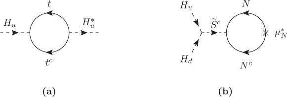
Figure 2: (a) A contribution to the radiatively induced effective Higgs potential by the top quarks in the MSSM. (b) A contribution to the radiatively induced effective Higgs potential by the singlets. It is compared with the diagram (a). The basic structures of the loops in (a) and (b) are the same. The trilinear scalar coupling in (b) comes from the cross term of $|\partial{W}/\partial{S}|^{2}$. Radiatively generated mass in the $\{N,N^{c}\}$ sector is transmitted to the Higgs through the mediation by $\widetilde{S}^{c}$.

The radiative correction $\Delta V(H)$ given with Eqs. (13) and (20) can be expanded in powers of $h_{u}$ and $h_{d}$ as follows:

$$\begin{split}\Delta V(H)=\Delta V^{\rm ren}_{(0,0)}+\Delta V^{\rm ren}_{(1,1)}h_{u}h_{d}+\frac{1}{2!2!}\left\{\Delta V^{\rm ren}_{(2,2)}+\Delta V^{\rm phy}_{(2,2)}\right\}(h_{u}h_{d})^{2}+\cdots,\end{split}$$ (21)

where the coefficients, $\Delta V^{\rm ren}_{(0,0)}$ [$\equiv\Delta V(H)|_{h_{u}=h_{d}=0}$], $\Delta V^{\rm ren}_{(1,1)}$ [$\equiv\partial_{h_{u}}\partial_{h_{d}}\Delta V(H)|_{h_{u}=h_{d}=0}$] and $\{\Delta V^{\rm ren}_{(2,2)}+\Delta V^{\rm phy}_{(2,2)}\}$ [$\equiv\partial^{2}_{h_{u}}\partial^{2}_{h_{d}}\Delta V(H)|_{h_{u}=h_{d}=0}$] are estimated as

$$\Delta V^{\rm ren}_{(0,0)}=\frac{n}{16\pi^{2}}\bigg{[}\left(\mu_{N}^{2}+\widetilde{m}_{N}^{2}\right)^{2}\left\{{\rm log}\left(\frac{\mu_{N}^{2}+\widetilde{m}_{N}^{2}}{\Lambda^{2}}\right)-\frac{3}{2}\right\}-\mu_{N}^{4}\left\{{\rm log}\left(\frac{\mu_{N}^{2}}{\Lambda^{2}}\right)-\frac{3}{2}\right\}\bigg{]},$$

$$\Delta V^{\rm ren}_{(1,1)}=\frac{-n}{8\pi^{2}}\left(y_{H}y_{N}\frac{\mu_{N}}{\mu_{S}}\right)\left[\left(\mu_{N}^{2}+\widetilde{m}_{N}^{2}\right)\left\{{\rm log}\left(\frac{\mu_{N}^{2}+\widetilde{m}_{N}^{2}}{\Lambda^{2}}\right)-1\right\}-\mu_{N}^{2}\left\{{\rm log}\left(\frac{\mu_{N}^{2}}{\Lambda^{2}}\right)-1\right\}\right],$$

$$\Delta V^{\rm ren}_{(2,2)}=\frac{n}{8\pi^{2}}\left(\frac{y_{H}y_{N}}{\mu_{S}}\right)^{2}\left[\left(\mu_{N}^{2}+\widetilde{m}_{N}^{2}\right)\left\{{\rm log}\left(\frac{\mu_{N}^{2}+\widetilde{m}_{N}^{2}}{\Lambda^{2}}\right)-1\right\}-\mu_{N}^{2}\left\{{\rm log}\left(\frac{\mu_{N}^{2}}{\Lambda^{2}}\right)-1\right\}\right],$$

$$\Delta V^{\rm phy}_{(2,2)}=\frac{n}{4\pi^{2}}\left(y_{H}y_{N}\frac{\mu_{N}}{\mu_{S}}\right)^{2}{\rm log}\left(\frac{\mu_{N}^{2}+\widetilde{m}_{N}^{2}}{\mu_{N}^{2}}\right).$$ (22)

Note that the coefficients of $h_{u}$, $h_{d}$, $h_{u}^{2}$, $h_{d}^{2}$, $h_{u}^{3}$, $h_{d}^{3}$, $h_{u}^{2}h_{d}$, and $h_{u}h_{d}^{2}$ in Eq. (21) are all zero, and the parts of “$\cdots$” are much suppressed by the higher powers of $(y_{H}y_{N}h_{u,d}^{2}/\mu_{S}\mu_{N})$. $\Delta V^{\rm ren}_{(0,0)}$ in Eqs. (21) or (III) just adds positive vacuum energy as seen from the first diagram of FIG. 1, which is a result of SUSY breaking.

As the (s-)top quark loops renormalize the soft mass squared of the Higgs, $m_{2}^{2}$ in the MSSM, the diagram of FIG. 2-(b) or $\Delta V^{\rm ren}_{(1,1)}$ term in Eq. (21) renormalizes the $B_{\mu}$ term in Eq. (19) ($B_{\mu}\mu\equiv m_{3}^{2}$), $m_{3}^{2}(\Lambda)=m_{3}^{2}-\Delta m_{3}^{2}$, where

$$\begin{split}\Delta m_{3}^{2}\approx\frac{n}{8\pi^{2}}\left(y_{H}y_{N}\frac{\mu_{N}}{\mu_{S}}\right)\left[\left(\mu_{N}^{2}+\widetilde{m}_{N}^{2}\right)\left\{{\rm log}\left(\frac{\mu_{N}^{2}+\widetilde{m}_{N}^{2}}{\Lambda^{2}}\right)-1\right\}-\mu_{N}^{2}\left\{{\rm log}\left(\frac{\mu_{N}^{2}}{\Lambda^{2}}\right)-1\right\}\right].\end{split}$$ (23)

Since $\widetilde{S}^{c}$ plays the role of the messenger relating $\{H_{u},H_{d}\}$ and $\{N,N^{c}\}$, the mass scale of $\widetilde{S}^{c}$ ($\approx\mu_{S}$) is the messenger scale for inducing $\Delta m_{3}^{2}$. Below the $\mu_{S}$ scale, thus, FIG. 2-(b) can effectively be a irreducible diagram, and $\Delta m_{3}^{2}$ in Eq. (23) can be regarded as a local operator. Hence, $\Delta m_{3}^{2}$ in Eq. (23) is valid below $\mu_{S}$, in which $\widetilde{S}^{c}$ as well as $\{N,N^{c}\}$ are decoupled. Thus, we set $\Lambda=\mu_{S}$ at lower energies.

With the correction Eq. (23), one of the tree-level extremum conditions in the Higgs potential is modified as

$$-2m_{3}^{2}=(m_{1}^{2}-m_{2}^{2})~{}{\rm tan}2\beta+M_{Z}^{2}~{}{\rm sin}2\beta-2\Delta m_{3}^{2}.$$ (24)

In order to avoid a fine-tuning among the parameters, $2\Delta m_{3}^{2}$ needs to be comparable with other terms in Eq. (24), when the parameters are chosen to explain the Higgs mass of 125 GeV. If $\Delta m_{3}^{2}$ is too large, it should be properly canceled by other terms, being equated with $M_{Z}^{2}{\rm sin}2\beta$ in Eq. (24). Then, the tuning is roughly estimated by the hierarchy, $M_{Z}^{2}~{}{\rm sin}2\beta/(2\Delta m_{3}^{2})$.

The $\Delta V^{\rm ren}_{(2,2)}$ term in Eq. (21), which renormalizes the $(\widetilde{m}^{2}_{S^{c}}/\mu_{S}^{2})y_{H}^{2}|H_{u}H_{d}|^{2}$ term in Eq. (19), originates from a quadratic term included in $\Delta V(\widetilde{S}^{c})$ in Eq. (13),

$$\begin{split}\frac{ny_{N}^{2}}{8\pi^{2}}\left[\left(\mu_{N}^{2}+\widetilde{m}_{N}^{2}\right)\left\{{\rm log}\left(\frac{\mu_{N}^{2}+\widetilde{m}_{N}^{2}}{\Lambda^{2}}\right)-1\right\}-\mu_{N}^{2}\left\{{\rm log}\left(\frac{\mu_{N}^{2}}{\Lambda^{2}}\right)-1\right\}\right]|\widetilde{S}^{c}|^{2},\end{split}$$ (25)

which contributes to renormalization of the tree-level soft mass term, $\widetilde{m}_{S^{c}}^{2}(\Lambda)|\widetilde{S}^{c}|^{2}$ in Eq. (LABEL:hsPot). Below the $\mu_{S}$ scale, $|\widetilde{S}^{c}|^{2}$ in Eq. (25) can be replaced by $(y_{H}/2\mu_{S})^{2}(h_{u}h_{d})^{2}$ as discussed before. The structure of Eq. (25) should be exactly the same as the radiative correction of $m_{2}^{2}$ in the MSSM Higgs sector by the (s-)tops loops, as seen from the similarity of the fourth diagram in FIG. 1 and FIG. 2-(a). The mass term of $\widetilde{S}^{c}$ in the scalar potential Eq. (LABEL:hsPot) is given by the summation of the above quadratic term Eq. (25) [$\equiv\delta\widetilde{m}^{2}_{S^{c}}(\Lambda)|\widetilde{S}^{c}|^{2}$], which comes from $\Delta V(\widetilde{S}^{c})$ in Eq. (13), and the tree-level soft mass term, which is also renormalization scale dependent. Inserting the RG solution of $\widetilde{m}^{2}_{S^{c}}$ in the tree-level soft mass squared $\widetilde{m}^{2}_{S^{c}}(\Lambda)$, $\widetilde{m}^{2}_{S^{c}}(\Lambda)+\delta\widetilde{m}^{2}_{S^{c}}(\Lambda)$ yields the low energy ($\Lambda<\mu_{N}$) value of the renormalized $\tilde{m}^{2}_{S^{c}}$ in its RG evolution CQW . As discussed already above Eq. (12), it was assumed to be relatively quite smaller than $\mu_{S}^{2}$ in Eq. (12):

$$\begin{split}\widetilde{m}^{2}_{S^{c}}(\Lambda=\mu_{S})+\delta\widetilde{m}^{2}_{S^{c}}(\Lambda=\mu_{S})\ll\mu_{S}^{2}.\end{split}$$ (26)

Note that the bosonic and fermionic modes of $\{N,N^{c}\}$ are all decoupled below the $\mu_{N}$ scale, and so $\widetilde{m}^{2}_{S^{c}}(\Lambda)+\delta\widetilde{m}^{2}_{S^{c}}(\Lambda)$ becomes frozen below $\mu_{N}$. Therefore, the $\Delta V^{\rm ren}_{(2,2)}$ term of Eq. (III) in the scalar potential ensures the smallness of the tree-level quartic term in Eq. (19) at the $\mu_{S}$ scale.

By comparing the quartic term, $\frac{1}{2!2!}\Delta V^{\rm phy}_{(2,2)}(h_{u}h_{d})^{2}$ in Eq. (21) with the scalar potential in the NMSSM, $V\supset\lambda^{2}|H_{u}H_{d}|^{2}=\frac{\lambda^{2}}{4}(h_{u}h_{d})^{2}$, one can see that $\Delta V^{\rm phy}_{(2,2)}$ in Eq. (III) plays the role of $\lambda^{2}$ of the NMSSM. Since we saw that the Higgs mass correction to the lightest Higgs mass in the NMSSM is given by $\lambda^{2}\times(v_{H}{\rm sin}2\beta)^{2}$ in Eq. (7), we can readily get the radiative correction $\Delta m_{h}^{2}$ in our case:

$$\begin{split}\Delta m_{h}^{2}\approx\frac{n}{4\pi^{2}}\left(y_{H}y_{N}\frac{\mu_{N}}{\mu_{S}}\right)^{2}\left(v_{H}^{2}{\rm sin}^{2}2\beta\right){\rm log}\left(\frac{\mu_{N}^{2}+\widetilde{m}_{N}^{2}}{\mu_{N}^{2}}\right).\end{split}$$ (27)

Note that $\mu_{S}$ originates from the propagator of $\widetilde{S}^{c}$ in the diagram, while $\mu_{N}$ from the mass insertion. Thus, the mass term correction by $\Delta m_{h}^{2}$ can be also a local operator below the messenger scale $\mu_{S}$. Since the mass squared of $\widetilde{S}^{c}$ [$>(300~{}{\rm GeV})^{2}$] is much heavier than the Higgs mass squared, $\Delta m_{h}^{2}$ in Eq. (27) indeed can be the Higgs mass correction at low energies. For discussion of the consistency of the model above the $\mu_{N}$ energy scale, one should return to Eq. (10), in which $y_{N}$ can be of order unity. By including Eq. (27), thus, the CP even lightest Higgs mass squared is modified as

$$\begin{split}m_{h}^{2}\approx M_{Z}^{2}{\rm cos}^{2}2\beta+\left\{\frac{\widetilde{m}_{S^{c}}^{2}}{\mu_{S}^{2}}-\frac{|A_{S}-B_{S}|^{2}}{\widetilde{m}_{S}^{2}+\mu_{S}^{2}}\right\}(y_{H}^{2}v_{H}^{2}{\rm sin}^{2}2\beta)+\Delta m_{h}^{2}|_{\rm MSSM}+\Delta m_{h}^{2}.\end{split}$$ (28)

Due to the hierarchy Eq. (12), the classical correction is suppressed.

As shown in Ref. KP , the Higgs mass of 125 GeV can be explained with Eqs. (28) or (27) in the parameter space,

$$\begin{split}0.2\lesssim y_{H}\lesssim 0.7\quad{\rm or}\quad 3\lesssim{\rm tan}\beta\lesssim 10,\end{split}$$ (29)

without the mixing effect, if the soft mass of the s-top is around 500 GeV [or $\Delta m_{h}^{2}|_{\rm MSSM}\approx(66~{}{\rm GeV})^{2}$]. Thus, even $0.2\lesssim y_{H}\lesssim 0.5$ or $3\lesssim{\rm tan}\beta\lesssim 10$, which is the excluded region in the NMSSM, can still be consistent with the 125 GeV Higgs mass, when the radiative correction of the Higgs mass is supported by the MSSM singlet fields.

For the typical three classes, $\mu_{S}\lesssim\widetilde{m}_{N}\lesssim\mu_{N}$ (Case A), $\mu_{S}\lesssim\mu_{N}\lesssim\widetilde{m}_{N}$ (Case B), and $\mu_{S}\lesssim\widetilde{m}_{N}\approx\mu_{N}$ (Case C), the radiative corrections in Eqs. (27) and (23) are approximated as follows:

$$\left\{\begin{array}[]{c}\Delta m_{h}^{2}\approx\frac{n}{4\pi^{2}}\left(v_{H}^{2}{\rm sin}^{2}2\beta\right)\left[\left(y_{H}y_{N}\frac{\mu_{N}}{\mu_{S}}\right)^{2}\frac{\widetilde{m}_{N}^{2}}{\mu_{N}^{2}}\right]\\ {\Delta m_{3}^{2}}\approx\frac{n}{4\pi^{2}}{\widetilde{m}_{N}^{2}}\left[\left(y_{H}y_{N}\frac{\mu_{N}}{\mu_{S}}\right){\rm log}\left(\frac{\mu_{N}}{\mu_{S}}\right)\right]\end{array}\right.\quad{\rm for}~{}~{}\widetilde{m}_{N}\lesssim\mu_{N}~{}~{}({\rm Case~{}A}),$$ (32)

$$\left\{\begin{array}[]{c}\Delta m_{h}^{2}\approx\frac{n}{4\pi^{2}}\left(v_{H}^{2}{\rm sin}^{2}2\beta\right)\left[\left(y_{H}y_{N}\frac{\mu_{N}}{\mu_{S}}\right)^{2}{\rm log}\left(\frac{\widetilde{m}_{N}^{2}}{\mu_{N}^{2}}\right)\right]\\ {\Delta m_{3}^{2}}\approx\frac{n}{4\pi^{2}}{\widetilde{m}_{N}^{2}}\left[\left(y_{H}y_{N}\frac{\mu_{N}}{\mu_{S}}\right){\rm log}\left(\frac{\widetilde{m}_{N}}{\mu_{S}}\right)\right]\end{array}\right.\quad{\rm for}~{}~{}\mu_{N}\lesssim\widetilde{m}_{N}~{}~{}({\rm Case~{}B}),$$ (35)

$$\left\{\begin{array}[]{c}\Delta m_{h}^{2}\approx\frac{n}{4\pi^{2}}\left(v_{H}^{2}{\rm sin}^{2}2\beta\right)\left[\left(y_{H}y_{N}\frac{\mu_{N}}{\mu_{S}}\right)^{2}{\rm log}2\right]\\ {\Delta m_{3}^{2}}\approx\frac{n}{4\pi^{2}}{\widetilde{m}_{N}^{2}}\left[\left(y_{H}y_{N}\frac{\mu_{N}}{\mu_{S}}\right)\left\{{\rm log}\left(2\frac{\mu_{N}}{\mu_{S}}\right)-\frac{1}{2}\right\}\right]\end{array}\right.\quad{\rm for}~{}~{}\mu_{N}\approx\widetilde{m}_{N}~{}~{}({\rm Case~{}C}).$$ (38)

In order to avoid a serious fine-tuning among the soft parameters in Eq. (24), $\Delta m_{3}^{2}/v_{H}^{2}$ should not be too much larger than unity. From the above equations, it roughly means $\widetilde{m}_{N}\lesssim 2\pi v_{H}\approx 1$ TeV. Hence, $\widetilde{m}_{N}$ should be quite smaller than 1 TeV. In the next section, we will discuss this issue in more detail.

IV 125 GeV Higgs Mass with the Least Tuning

In this section, we study the least tuning condition, under which the tuning in the Higgs sector is minimized for a given $\Delta m_{h}^{2}$. For simple presentations, we parametrize the radiative corrections in Eqs. (27) and (23) as follows:

$$\begin{split}&\qquad\qquad\qquad\qquad F^{2}\equiv\frac{\Delta m_{h}^{2}}{f^{2}v_{H}^{2}}=R^{2}~{}{\rm log}\left(1+r^{2}\right),\\ &G\equiv\frac{2\Delta m_{3}^{2}}{g\mu_{S}^{2}}=R^{3}\left[\left(1+r^{2}\right)\left\{{\rm log}(1+r^{2})+{\rm log}R^{2}-1\right\}-\left\{{\rm log}R^{2}-1\right\}\right],\end{split}$$ (39)

where $R$, $r$, and $f^{2}$, $g$ are defined as

$$\begin{split}&~{}~{}~{}~{}~{}~{}R\equiv\frac{\mu_{N}}{\mu_{S}}~{},\quad r\equiv\frac{\widetilde{m}_{N}}{\mu_{N}}~{},\quad{\rm and}\\ &f^{2}\equiv\frac{n}{4\pi^{2}}y_{H}^{2}y_{N}^{2}{\rm sin}^{2}2\beta~{},\quad g\equiv\frac{n}{4\pi^{2}}y_{H}y_{N}.\end{split}$$ (40)

For the parameters chosen for the explanation of the Higgs mass around 125 GeV, as mentioned above, a smaller $\Delta m_{3}^{2}$ is more desirable to avoid a fine-tuning among the parameters in Eq. (23). From now on, we will explore the conditions under which $\Delta m_{3}^{2}$ can be minimized for a given $\Delta m_{h}^{2}$ and other parameters in the model. As seen from Eq. (LABEL:FG), $R$ and $r$ are related to each other for a given $F$. Accordingly, $G$ depends only on $r$ or $R$ for a fixed $F$. Let us insert $F$ into $G$, replacing $r$ by $R$ and $F$. For a given set of $\{\Delta m_{h}^{2},\mu_{S}^{2},f^{2},g\}$, thus, $G$ is recast as

$$\begin{split}G=R^{3}\left[e^{\frac{F^{2}}{R^{2}}}\left(\frac{F^{2}}{R^{2}}+{\rm log}R^{2}-1\right)-\left({\rm log}R^{2}-1\right)\right].\end{split}$$ (41)

Provided that $F$ is fixed, one can show that $G$ is minimized at

$$\begin{split}R=\frac{F}{1+\epsilon_{F}}\end{split}$$ (42)

where the small parameter $\epsilon_{F}$ is estimated as

$$\begin{split}\epsilon_{F}\approx\frac{1-0.28~{}{\rm log}F^{2}}{8.87+4.31~{}{\rm log}F^{2}}.\end{split}$$ (43)

$|\epsilon_{F}|$ is much smaller than unity in the most parameter range of $F$: $|\epsilon_{F}|$ is smaller than $0.3$ ($0.1$) for $0<|F|<0.16$ or $0.59<|F|$ ($0<|F|<1.9\times 10^{-3}$ or $1.08<|F|$). From Eq. (LABEL:FG), thus, $r$ and $G$ are determined when $G$ minimized:

$$\begin{split}&\qquad\qquad~{}~{}~{}r^{2}\approx 1.72+5.44\epsilon_{F},\\ &G\approx F^{3}\left[(1.72+0.28\epsilon_{F})~{}{\rm log}F^{2}+(1-\epsilon_{F})\right].\end{split}$$ (44)

For instance, $\epsilon_{F}\approx 0.05$, $R\approx 1.75$, $r\approx 1.35$, and $G\approx 19.09$ for $F=1.84$. From Eq. (LABEL:def), it implies that $\frac{\mu_{N}}{\mu_{S}}\approx 1.75$, $\frac{\widetilde{m}_{N}}{\mu_{N}}\approx 1.35$, and $\Delta m_{3}^{2}\approx(330~{}{\rm GeV})^{2}$ e.g. for $|\Delta m_{h}|=91$ GeV, $\mu_{S}=300$ GeV, $n=5$, $y_{H}y_{N}=1$, and ${\rm sin}2\beta=0.8$.

Note that $0.3<r<1.8$ for $-0.3<\epsilon_{F}<0.3$ in Eq. (LABEL:minm). We can see that $\mu_{N}$ and $\widetilde{m}_{N}$ need to be comparable to each other in order to minimize $\Delta m_{3}^{2}$. However, $\Delta m_{3}^{2}$ is not much sensitive to $\widetilde{m}_{N}/\mu_{N}$ ($=r$), only if $\widetilde{m}_{N}/\mu_{N}$ is larger than unity, because $r$ logarithmically depends on the constraint relation associated with $F$ in Eq. (LABEL:FG).

In Eq. (LABEL:minm), $G$ could be further minimized with a small $F$. Since $\Delta m_{h}^{2}\approx m_{h}^{2}-M_{Z}^{2}{\rm cos}^{2}2\beta-\Delta m_{h}^{2}|_{\rm MSSM}$, $F^{2}$ in Eq. (LABEL:FG) is minimized when ${\rm sin}^{2}2\beta=1$ (or ${\rm tan}\beta=1$):

$$\begin{split}F^{2}\approx\frac{m_{h}^{2}-M_{Z}^{2}-\Delta m_{h}^{2}|_{\rm MSSM}+M_{Z}^{2}~{}{\rm sin}^{2}2\beta}{\frac{n}{4\pi^{2}}(y_{H}y_{N})^{2}v_{H}^{2}~{}{\rm sin}^{2}2\beta}\geq\frac{m_{h}^{2}-\Delta m_{h}^{2}|_{\rm MSSM}}{\frac{n}{4\pi^{2}}(y_{H}y_{N})^{2}v_{H}^{2}}~{},\end{split}$$ (45)

For $n=5$, $(y_{H}y_{N})=1$, and $\Delta m_{h}^{2}|_{\rm MSSM}=(66~{}{\rm GeV})^{2}$ [which corresponds to $\widetilde{m}_{t}\approx 500$ GeV at two-loop level], thus, the minimum of $F^{2}$ is $(1.71)^{2}$, which gives $G\approx 14.07$ or $\Delta m_{3}^{2}\approx(284~{}{\rm GeV})^{2}$. To avoid another fine-tuning needed for minimizing the tuning, however, we do not rigorously apply the least tuning condition. Nonetheless, the tuning problem associated with the extremum conditions can still be remarkably mitigated with relatively smaller $\Delta m_{3}^{2}$, compared to the MSSM. For $\Delta m_{3}^{2}$ with other parameters, see FIG. 3 and 4. Note that even the soft parameters much lighter than 500 GeV can explain the Higgs mass of 125 GeV. Taking such light mass parameters is not in conflict with the LHC experimental results unlike the extra matter scenario. It is possible because the newly introduced particles are MSSM singlets.

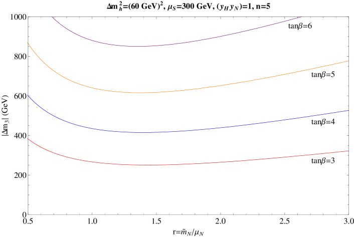
Figure 3: Radiative correction $|\Delta m_{3}|$ ($\equiv\sqrt{B_{\mu}\mu}$) vs. $\widetilde{m}_{N}/\mu_{N}$ for various values of ${\rm tan}\beta$. The radiative correction to the Higgs mass $\Delta m_{h}^{2}$ is set to $(60~{}{\rm GeV})^{2}$. By $|\Delta m_{h}|_{\rm MSSM}\approx(68,70,75,82)$ GeV for ${\rm tan}\beta=(6,5,4,3)$, thus, the Higgs mass get additional contributions from the (s-)top to be 125 GeV. They correspond to $\widetilde{m}_{t}\approx(530,590,780,1300)$ GeV at two-loop level, when turning off the mixing effect of $({\tilde{t}_{L},\tilde{t}_{R}})$ and the tree-level $|H_{u}H_{d}|^{2}$ terms in Eq. (19). We fix the other parameters as shown in the figure.

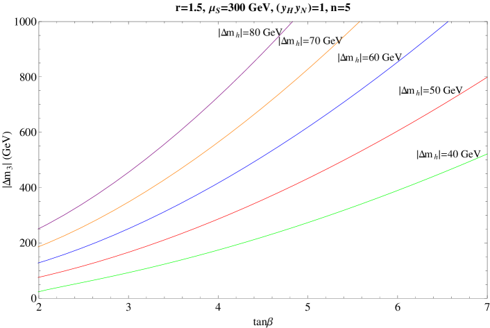
Figure 4: Radiative correction $|\Delta m_{3}|$ ($\equiv\sqrt{B_{\mu}\mu}$) vs. ${\rm tan}\beta$ for various values of $\Delta m_{h}^{2}$ around the least tuning points ($\widetilde{m}_{N}/\mu_{N}\approx 1.5$). $|\Delta m_{h}|=(80,70,60,50,40)$ GeV for ${\rm tan}\beta=5$ require the supplements of $|\Delta m_{h}|_{\rm MSSM}\approx(47,61,70,78,83)$ GeV, respectively, by the (s-)top’s contributions. They correspond to $\widetilde{m}_{t}\approx(230,390,590,940,1400)$ GeV at two-loop level, when turning off the mixing effect of $({\tilde{t}_{L},\tilde{t}_{R}})$ and the tree-level $|H_{u}H_{d}|^{2}$ terms in Eq. (19). The other parameters are fixed as shown in the figure.

Let us present the estimates of typical values of $\Delta m_{3}^{2}$ for the three classes defined in section III, when $\Delta m_{h}^{2}$ and other parameters are given. In Case A, namely, for $\widetilde{m}_{N}\lesssim\mu_{N}$, we have

$$\qquad\qquad\qquad\Delta m_{3}^{2}\approx\mu_{S}^{2}\left[\frac{|\Delta m_{h}|}{v_{H}}\right]^{3}\frac{g}{f^{3}r}~{}{\rm log}\left(\frac{|\Delta m_{h}|}{fv_{H}r}\right)$$ (46)

$$\approx(592~{}{\rm GeV})^{2}\left[\frac{\mu_{S}}{300~{}{\rm GeV}}\right]^{2}\left[\frac{|\Delta m_{h}|}{90~{}{\rm GeV}}\right]^{3}\left[\frac{1.14}{\sqrt{n}(y_{H}y_{N})^{2}{\rm sin}^{3}2\beta}\right]\left[\frac{\frac{1}{r}~{}{\rm log}\left(\frac{|\Delta m_{h}|}{fv_{H}r}\right)}{3~{}{\rm log}\left(\frac{3\cdot 90}{0.28\cdot 174}\right)}\right].$$

In Case B, i.e. for $\mu_{N}\lesssim\widetilde{m}_{N}$,

$$\qquad\qquad\qquad\Delta m_{3}^{2}\approx\mu_{S}^{2}\left[\frac{|\Delta m_{h}|}{v_{H}}\right]^{3}\frac{gr^{2}}{f^{3}({\rm log}r^{2})^{3/2}}~{}{\rm log}\left(\frac{r|\Delta m_{h}|}{\sqrt{{\rm log}r^{2}}fv_{H}}\right)$$ (47)

$$\approx(499~{}{\rm GeV})^{2}\left[\frac{\mu_{S}}{300~{}{\rm GeV}}\right]^{2}\left[\frac{|\Delta m_{h}|}{90~{}{\rm GeV}}\right]^{3}\left[\frac{1.14}{\sqrt{n}(y_{H}y_{N}){\rm sin}^{3}2\beta}\right]\left[\frac{\frac{r^{2}}{({\rm log}r^{2})^{3/2}}~{}{\rm log}\left(\frac{r|\Delta m_{h}|}{\sqrt{{\rm log}r^{2}}fv_{H}}\right)}{2.76~{}{\rm log}\left(\frac{3\cdot 90}{1.48\cdot 0.28\cdot 174}\right)}\right].$$

In Case C, i.e. for $\mu_{N}\approx\widetilde{m}_{N}$,

$$\qquad\quad\quad\Delta m_{3}^{2}\approx\mu_{S}^{2}\left[\frac{|\Delta m_{h}|}{v_{H}}\right]^{3}\frac{g}{f^{3}({\rm log}2)^{3/2}}\left[{\rm log}\left(\frac{2|\Delta m_{h}|}{fv_{H}\sqrt{{\rm log}2}}\right)-\frac{1}{2}\right]$$ (48)

$$\approx(342~{}{\rm GeV})^{2}\left[\frac{\mu_{S}}{300~{}{\rm GeV}}\right]^{2}\left[\frac{|\Delta m_{h}|}{90~{}{\rm GeV}}\right]^{3}\left[\frac{1.14}{\sqrt{n}(y_{H}y_{N})^{2}{\rm sin}^{3}2\beta}\right]\left[\frac{{\rm log}\left(\frac{2|\Delta m_{h}|}{fv_{H}\sqrt{{\rm log}2}}\right)-\frac{1}{2}}{0.99}\right].$$

V Diphoton Decay Enhancement

According to the reports by the CMS and ATLAS CMS ; ATLAS , they both have observed an excess in the Higgs production and decay to the diphoton channel, which is about 1.5 – 2 times larger than the SM expectation. On the other hand, the $ZZ$ and $WW$ channels are quite compatible with the SM:

$$\begin{split}&\frac{\sigma(gg\rightarrow h)\times{\rm Br}(h\rightarrow\gamma\gamma)}{[\sigma(gg\rightarrow h)\times{\rm Br}(h\rightarrow\gamma\gamma)]_{\rm SM}}\sim 1.5-2,\\ &~{}\quad\frac{\sigma(gg\rightarrow h)\times{\rm Br}(h\rightarrow VV)}{[\sigma(gg\rightarrow h)\times{\rm Br}(h\rightarrow VV)]_{\rm SM}}\sim 1,\end{split}$$ (49)

where $V$ indicates $Z$ or $W$. In fact, the excess at 8 TeV of the LHC slightly decreases compared to that for 7 TeV. However, if the large excess in the diphoton decay channel persists even after further more precise analyses with more data, one must seriously consider the possibility of the presence of new charged particles at low energies C ; A .

So far, we have regarded $\{N,N^{c}\}$ as vectorlike $n$-dimensional representations of a hidden gauge group. In this section, however, by slightly modifying the model, namely, assigning additional electromagnetic (or hyper) charges, $Q_{N}$ and $-Q_{N}$, respectively to $N$ and $N^{c}$, we attempt to explain the excess of the diphoton decay rate of the Higgs under the assumption that the enhanced diphoton decay rate of the Higgs will survive. Thus, the mechanism of the Higgs mass enhancement and mitigating the fine-tuning can be closely associated with the excess of the diphoton decay rate of the Higgs in our framework. Since $\{N,N^{c}\}$ do not carry any SU(3)_c and SU(2)_L quantum numbers, they would not affect the Higgs production rate at the LHC $gg\rightarrow h$, and decay rate $h\rightarrow WW$. Also they do not much perturb the tree-level decay rate of $h\rightarrow ZZ$. With $\{N,N^{c}\}$ carrying U(1)_Y charges, however, the gauge coupling unification in the MSSM is spoiled, unless an exotic normalization of U(1)_Y is supported in a UV theory. It is the cost for the explanation of the diphoton excess of the Higgs.

As discussed in Ref. C , e.g. by extra vectorlike charged leptons, the sizable enhancement of $h\rightarrow\gamma\gamma$ can be successfully achieved, if the coefficient of the dimension five interaction between the Higgs boson and the fermion, $(c_{f}/\Lambda)H^{\dagger}H\bar{f}f$ is negative. We can obtain a similar operator by integrating out $\widetilde{S}^{c}$ in our framework:

$$\begin{split}-{\cal L}_{\rm eff}=-\frac{y_{H}y_{N}}{\mu_{S}}H_{u}H_{d}NN^{c}~{}~{}+~{}~{}{\rm h.c.}.\end{split}$$ (50)

Here $N$, $N^{c}$ are the fermionic modes of the superfields $\{N,N^{c}\}$ (Weyl fermions). They form a Dirac fermion, $f=(N,N^{c*})^{T}$. Thus, $\{N,N^{c}\}$ get an additional mass coming from the Higgs’ vacuum expectation values (VEVs) apart from the bare mass $\mu_{N}$:

$$\begin{split}M_{N}\approx\mu_{N}-y_{H}y_{N}\frac{v_{u}v_{d}}{\mu_{S}},\end{split}$$ (51)

where $v_{u,d}\equiv\langle H_{u,d}\rangle$. It can also be obtained from Eq. (14) and the solution of $\widetilde{S}^{c}$ in Eq. (LABEL:ScS). Connecting the $N$, $N^{c}$ lines in Eq. (50), the operator associated with the diagram in FIG. 2-(b) is reproduced. The relevant diagram for $h\rightarrow\gamma\gamma$ is obtained by attaching two photons to the loops. Of course, the bosonic modes of $\{N,N^{c}\}$ also make a contribution to $h\rightarrow\gamma\gamma$. However, they less affect the decay, since they are relatively heavier than the fermionic partners. With Eqs. (50) and (51), the enhancement factor over the SM diphoton width C is estimated in the heavy Higgs decoupling limit as follows:

$$\begin{split}R_{\gamma\gamma}\approx\left|1-\frac{y_{H}y_{N}}{\sqrt{2}}\frac{v_{H}^{2}{\rm sin}2\beta}{\mu_{S}M_{N}}\frac{nQ^{2}_{N}\left\{A_{1/2}(x_{N})+{\cal O}\left(\frac{m_{h}}{\widetilde{m}_{N}}\right)\right\}}{A_{1}(x_{W})+3\left(\frac{2}{3}\right)^{2}A_{1/2}(x_{t})}\right|^{2},\end{split}$$ (52)

where $x_{i}\equiv 4m_{i}^{2}/m_{h}^{2}$. $n$ denotes the dimension of the representation of $\{N,N^{c}\}$ under a hidden gauge group, and $(-)Q_{N}$ means the electromagnetic charge $N$ ($N^{c}$) carries. Below the $WW$ threshold, the loop functions for the vector boson ($A_{1}$) and the fermion ($A_{1/2}$) are given by

$$\begin{split}&A_{1}(x)=-x^{2}\left[2x^{-2}+3x^{-1}+3\left(2x^{-1}-1\right)f(x^{-1})\right],\\ &\qquad A_{1/2}(x)=2x^{2}\left[x^{-1}+\left(x^{-1}-1\right)f(x^{-1})\right],\end{split}$$ (53)

where $f(x^{-1})\equiv{\rm arcsin}^{2}x^{-1/2}$. We ignore the contributions by the bosonic partners in $\{N,N^{c}\}$, which is just of order ${\cal O}\left(m_{h}/\widetilde{m}_{N}\right)$, because of their relatively heavier masses.

The main SM contributions, $A_{1}(x_{W})$ by the $W$ boson and $3(\frac{2}{3})^{2}A_{1/2}(x_{t})$ by the top quark, which appear in the denominator of Eq. (52) are $-8.32$ and $1.84$, respectively. For constructive interference, thus, the sign of $(y_{H}y_{N}/\mu_{S}M_{N})$ should be positive. See FIG. 5, in which we display the contour plots for the enhancement factor over the SM diphoton width in the $M_{N}$–$Q_{N}$ plane for the $n=5$ and $n=1$ cases.

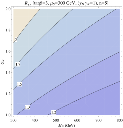
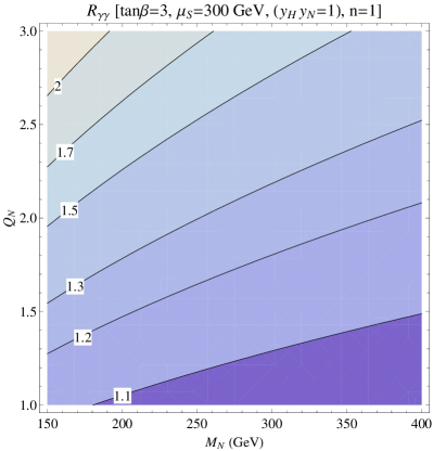
Figure 5: Contour plots for the enhancement factor over the SM diphoton width in the $M_{N}$–$Q_{N}$ plane. We fix the other parameters as shown in each figure.

Only with Eq. (10), a considerable amount of $\{N,N^{c}\}$ would remain as cosmological relic, unless the reheating temperature is very low, which is a disaster when they carry electromagnetic charges. To avoid it, we discuss two possibilities here. One could consider the possibility that $N$, $N^{c}$ condense by the strong hidden gauge interaction as the quarks in QCD. Then, only the neutral hadron would remain in our case, and it can decay to the two photons as the pion $\pi^{0}$ in QCD. In this case, $M_{N}$ in Eq. (52) should be replaced by $8\pi^{2}f_{N}/3$, where $f_{N}$ is the decay constant determined by confining of the hidden gauge interaction. Alternatively, if $n=1$ and $Q_{N}=-2$, the superpotential allows the interactions with the MSSM charged lepton singlets, $N(e^{c})^{2}$. Then, $N$, $N^{c}$, and $\widetilde{N}$, $\widetilde{N}^{c}$ can decay eventually to $e^{\pm}$ and the neutralinos before nucleosynthesis starts even without the assumption of the hidden confining gauge interaction.

VI The Model

As mentioned in section II, the superpotential Eq. (10) should be embedded in the superpotential of a UV model, which permits more global symmetries. The singlets $S$ and $S^{c}$ should be charged under the global symmetries to avoid the tadpole problem associated with pure singlets tadpole1 ; tadpole2 . The global symmetries should be broken such that there is no remaining PQ symmetry at low energies, explaining the desired sizes of $\mu$, $\mu_{S}$, and $\mu_{N}$ in Eq. (10). If the PQ symmetry is broken at the scale of $\sqrt{m_{3/2}M_{P}}$ ($\sim 10^{10}$ GeV), the tadpole problem could be avoided tadpole1 ; JSY .

The effective superpotential Eq. (10) can be deduced e.g. from the following UV K${\rm\ddot{a}}$hler potential and the superpotential:

$$\begin{split}&\qquad\quad~{}~{}K_{\rm UV}\supset\kappa\frac{X^{\dagger}}{M_{P}}SS^{c}~{}~{}+~{}~{}{\rm h.c.}\,,\\ &\qquad\quad W_{\rm UV}=y_{H}SH_{u}H_{d}+y_{N}S^{c}NN^{c}\\ &+\frac{\lambda_{1}}{M_{P}}\Sigma_{1}^{2}H_{u}H_{d}+\frac{\lambda_{2}}{M_{P}}\Sigma_{2}^{2}NN^{c}+\frac{\lambda_{3}}{M_{P}}\Sigma_{1}\Sigma_{2}\overline{\Sigma}^{2},\\ \end{split}$$ (54)

where $y_{H}$, $y_{N}$, $\kappa$ and $\lambda_{i}$ ($i=1,2,3$) are dimensionless couplings, and $M_{P}$ denotes the reduced Planck mass ($=2.4\times 10^{18}$ GeV). The K${\rm\ddot{a}}$hler potential and the superpotential Eq. (LABEL:UV) respect the global symmetry, U(1)${}_{\rm R}\times$U(1)_PQ. The global charges for the superfields are displayed in TABLE I.

Superfields	$H_{u}$	$H_{d}$	$N$	$N^{c}$	$S$	$S^{c}$	$\Sigma_{1}$	$\Sigma_{2}$	$\overline{\Sigma}$	$X$
U(1)R	$0$	$0$	$0$	$0$	$2$	$2$	$1$	$1$	$0$	$4$
U(1)PQ	$-\frac{1}{4}$	$-\frac{1}{4}$	$\frac{1}{2}$	$\frac{1}{2}$	$\frac{1}{2}$	$-1$	$\frac{1}{4}$	$-\frac{1}{2}$	$\frac{1}{8}$	$-\frac{1}{2}$

Table 1: R and Pecci-Quinn charges of the superfields. The MSSM matter superfields carry unit R charges, and also PQ charges of $1/8$. $N$ and $N^{c}$ are assumed to be proper $n$-dimensional vectorlike representations of a hidden gauge group, under which all the MSSM fields are neutral.

The $F$-component of the superfield $X$ is assumed to develop a VEV of order $m_{3/2}M_{P}$, breaking SUSY. Thus, the $\mu_{S}$ term of order $m_{3/2}$ in Eq. (10) can be generated from the K${\rm\ddot{a}}$hler potential Eq. (LABEL:UV) GM . By the “$A$-term” corresponding to the $\lambda_{3}$ terms in Eq. (LABEL:UV) and the soft mass terms in the scalar potential, the VEVs of $\Sigma_{1,2}$ and $\overline{\Sigma}$ of order $\sqrt{m_{3/2}M_{P}}$ ($\sim 10^{10}$ GeV) are generated at the minimum 422 . From the $\lambda_{1,2}$ terms in Eq. (LABEL:UV), thus, “$\mu$” in the MSSM, and also $\mu_{N}$ in Eq. (10), which are also of order $m_{3/2}$ Kim-Nilles , are generated.

The global symmetries are broken by the SUSY breaking effects: by the VEV of the $F$-component of $X$, the U(1)_R symmetry is broken to $Z_{2}$, which is identified with the matter parity in the MSSM, and due to the VEVs of $\{\Sigma_{1,2},\overline{\Sigma}\}$, U(1)_PQ are completely broken at the intermediate scale. Note that a tadpole term of $S^{c}$ in the superpotential can be induced after the global symmetries are broken [$W\supset S^{c}(\langle\overline{\Sigma}\rangle)^{8}/M_{P}^{6}\sim S^{c}m_{3/2}^{4}/M_{P}^{2}$], but it is extremely suppressed. Since $\Sigma_{1,2}$ and $\overline{\Sigma}$ carry accidental $Z_{2}\times Z_{2}^{\prime}$ charges of $(1,0)$ and $(0,1)$, respectively, a domain wall problem would potentially arise. Hence, we assume that the discrete symmetries were already broken before or during inflation such that domain walls were diluted away. If the reheating temperature is lower than $10^{9}$ GeV, the $Z_{2}\times Z_{2}^{\prime}$ breaking vacuum can still be the minimum of the potential also after inflation 422 .

Finally, let us discuss the tadpole problem tadpole1 in this case. The K${\rm\ddot{a}}$hler potential e.g. for the Higgs fields takes the following form:

$$\begin{split}K_{\rm UV}\supset\sum_{i=u,d}H_{i}H_{i}^{\dagger}+\frac{\alpha_{i}H_{i}H_{i}^{\dagger}}{M_{P}}\left\{S\left(\frac{\Sigma_{1}^{\dagger}}{M_{P}}\right)^{2}+{\rm h.c.}\right\}+\frac{\beta_{i}H_{i}H_{i}^{\dagger}}{M_{P}}\left\{S^{c}\left(\frac{\Sigma_{2}^{\dagger}}{M_{P}}\right)^{2}+{\rm h.c.}\right\},\end{split}$$ (55)

which is consistent with the quantum numbers listed in TABLE I. Note that $(\Sigma_{1,2}^{\dagger}/M_{P})^{2}$ are accompanied with $S^{(c)}$ in Eq. (55), since $S$, $S^{c}$ carry the global charges. They effectively suppress the coefficients $\alpha_{i}$ and $\beta_{i}$ with $(\langle\widetilde{\Sigma}_{1,2}\rangle/M_{P})^{2}\sim m_{3/2}/M_{P}$. When SUSY is broken in the hidden sector, thus, the scalar potential and kinetic terms in SUGRA with Eq. (55) are recast into

$$\begin{split}&V_{\rm vis.}=K^{ij*}W_{i}W_{j}^{*}+m_{3/2}^{2}K^{ij*}K_{i}K_{j*}+{\cal O}\left(\frac{m_{3/2}^{2}}{M_{P}^{2}}\right)\\ &\supset\sum_{i=u,d}|H_{i}|^{2}\frac{m_{3/2}^{3}}{M_{P}^{2}}\bigg{[}\alpha_{i}^{\prime}\left\{\widetilde{S}+\widetilde{S}^{*}\right\}+\beta_{i}^{\prime}\left\{\widetilde{S}^{c}+\widetilde{S}^{c*}\right\}\bigg{]},\end{split}$$ (56)

where superscripts and subscripts in the K${\rm\ddot{a}}$hler and superpotential denote differentiations with respect to the scalar fields in SUGRA, and

$$\begin{split}&{\cal L}_{\rm kin.}=K_{ij*}\partial_{\mu}z^{i}\partial^{\mu}z^{j*}\supset\sum_{i=u,d}|\partial_{\mu}H_{i}|^{2}\frac{m_{3/2}}{M_{P}^{2}}\bigg{[}\alpha_{i}^{\prime}\left\{\widetilde{S}+\widetilde{S}^{*}\right\}+\beta_{i}^{\prime}\left\{\widetilde{S}^{c}+\widetilde{S}^{c*}\right\}\bigg{]}.\end{split}$$ (57)

$|H_{i}|^{2}$ in Eq. (LABEL:Vsinglet) and $|\partial_{\mu}H_{i}|^{2}$ in Eq. (LABEL:Lsinglet) introduce quadratic divergences in the loop integrals, inducing the tadpole terms of $\widetilde{S}$ and $\widetilde{S}^{c}$ in the Lagrangian,

$$\begin{split}\Lambda_{\rm cutoff}^{2}~{}\frac{m_{3/2}^{3}}{M_{P}^{2}}\left\{\widetilde{S}^{(c)}+\widetilde{S}^{(c)*}\right\},\end{split}$$ (58)

where we dropped the numerical factors. Even if $\Lambda_{\rm cutoff}^{2}=M_{P}$, thus, the tadpole coefficients are just of order $m_{3/2}$ or smaller. With the minimal K${\rm\ddot{a}}$hler potential, moreover, such divergences are known to be canceled out at the one-loop level Jain . Accordingly, the shifts of the VEVs by the tadpoles, $\langle\delta\widetilde{S}\rangle$ and $\langle\delta\widetilde{S}^{c}\rangle$ are quite suppressed in our case, and so the gauge hierarchy is not destabilized by them. In this paper, hence, we neglect their effects. Note that were it not for the global symmetries, $(\Sigma_{1,2}^{\dagger}/M_{P})^{2}$ are absent in Eq. (55). Without the factors, we had extremely huge tadpole terms, $\Lambda_{\rm cutoff}^{2}\frac{m_{3/2}^{2}}{M_{P}}\{\widetilde{S}^{(c)}+\widetilde{S}^{(c)*}\}$, which destabilizes the gauge hierarchy, since $S$ couples to $H_{u}$ and $H_{d}$ at the tree level in the superpotential Eq. (10) tadpole1 .

VII Conclusion

We proposed a new type of the singlet extension of the MSSM in order to raise the Higgs mass to 125 GeV with the alleviation of the tuning associated with the light Higgs mass. Apart from the (s-)top quark’s contribution, the Higgs mass is radiatively generated in a hidden sector because of the mass splitting of hidden sector fields, and such an effect is transmitted to the Higgs sector through the mediation by the messenger field $\widetilde{S}^{c}$. Since the Higgs mass is raised by the superpotential parameters, lifting the Higgs mass is quite efficient as in the extra matter scenario. Unlike the extra matter scenario, however, our model is free from the constraint on extra colored particles with order-one Yukawa couplings to the Higgs, which is associated with the production and decay rates of the Higgs at the LHC 4thfamily .

As shown in our previous paper KP , the parameter space for 125 GeV Higgs mass can be enlarged compared to the original form of the NMSSM, and so even $0.2\lesssim y_{H}\lesssim 0.5$ or $3\lesssim{\rm tan}\beta\lesssim 10$, which is excluded region in the NMSSM, can explain the 125 GeV Higgs mass with a relatively light s-top ($\sim 500$ GeV) but without considering the mixing effect. In this paper, we also particularly emphasized that the fine-tuning problem associated with the light Higgs mass can be remarkably mitigated by taking low enough messenger scale ($\approx 300$ GeV) and light enough mass parameters ($\ll 1$ TeV). We have explored the least tuning condition ($\mu_{N}\lesssim\widetilde{m}_{N}$), under which even the soft parameters much lighter than 500 GeV can explain the Higgs mass of 125 GeV without conflicting with the LHC experimental results. It is possible because the newly introduced particles are MSSM singlets.

Under the assumption that the observed excess of the diphoton decay rate of the Higgs over the SM expectation will persist, we also studied the way to enhance the diphoton decay rate in our framework. It turns out to be simply realized, only if the hidden sector fields in our model are converted to carry also electromagnetic charges. Thus, the mechanism of the Higgs mass enhancement and mitigating the fine-tuning can be closely related to the excess of the diphoton decay rate of the Higgs in our framework.

- (1) S. Chatrchyan et al. [CMS Collaboration], Phys. Lett. B 716, 30 (2012) [arXiv:1207.7235 [hep-ex]]; see also 710, 26 (2012) [arXiv:1202.1488 [hep-ex]].
- (2) G. Aad et al. [ATLAS Collaboration], Phys. Lett. B 716, 1 (2012) [arXiv:1207.7214 [hep-ex]]; see also 710, 49 (2012) [arXiv:1202.1408 [hep-ex]].
- (3) For a review, see A. Djouadi, Phys. Rept. 459, 1 (2008).
- (4) See, for instance, K. -S. Choi and B. Kyae, Nucl. Phys. B 855, 1 (2012) [arXiv:1102.0591 [hep-th]]; J. -H. Huh, J. E. Kim and B. Kyae, Phys. Rev. D 80, 115012 (2009) [arXiv:0904.1108 [hep-ph]]; J. E. Kim, J. -H. Kim and B. Kyae, JHEP 0706, 034 (2007) [hep-ph/0702278 [hep-ph]]; J. E. Kim and B. Kyae, Nucl. Phys. B 770, 47 (2007) [hep-th/0608086].
- (5) M. S. Carena and H. E. Haber, Prog. Part. Nucl. Phys. 50, 63 (2003); see also G. F. Giudice and A. Strumia, Nucl. Phys. B 858, 63 (2012).
- (6) T. Moroi and Y. Okada, Mod. Phys. Lett. A 7, 187 (1992); T. Moroi and Y. Okada, Phys. Lett. B 295, 73 (1992); K. S. Babu, I. Gogoladze and C. Kolda, hep-ph/0410085; K. S. Babu, I. Gogoladze, M. U. Rehman and Q. Shafi, Phys. Rev. D 78, 055017 (2008); S. P. Martin, Phys. Rev. D 81, 035004 (2010).
- (7) T. Moroi, R. Sato and T. T. Yanagida, Phys. Lett. B 709, 218 (2012).
- (8) E. Kuflik, Y. Nir and T. Volansky, arXiv:1204.1975 [hep-ph]; see also N. Chen and H. -J. He, JHEP 1204, 062 (2012) [arXiv:1202.3072 [hep-ph]].
- (9) B. Kyae and J. -C. Park, Phys. Rev. D 86, 031701 (2012) [arXiv:1203.1656 [hep-ph]].
- (10) For a review, see U. Ellwanger, C. Hugonie and A. M. Teixeira, Phys. Rept. 496, 1 (2010).
- (11) U. Ellwanger, JHEP 1203, 044 (2012) [arXiv:1112.3548 [hep-ph]]; S. F. King, M. Muhlleitner and R. Nevzorov, Nucl. Phys. B 860, 207 (2012) [arXiv:1201.2671 [hep-ph]]; Z. Kang, J. Li and T. Li, JHEP 1211, 024 (2012) [arXiv:1201.5305 [hep-ph]]; J. Cao, Z. Heng, J. M. Yang, Y. Zhang and J. Zhu, JHEP 1203, 086 (2012) [arXiv:1202.5821 [hep-ph]]; U. Ellwanger and C. Hugonie, Adv. High Energy Phys. 2012, 625389 (2012) [arXiv:1203.5048 [hep-ph]].
- (12) For other types of singlet extensions of the (MS)SM, see, for instance, A. Delgado, C. Kolda, J. P. Olson and A. de la Puente, Phys. Rev. Lett. 105, 091802 (2010) [arXiv:1005.1282 [hep-ph]]; G. G. Ross and K. Schmidt-Hoberg, Nucl. Phys. B 862, 710 (2012) [arXiv:1108.1284 [hep-ph]].
- (13) J. E. Kim, H. P. Nilles and M. -S. Seo, Mod. Phys. Lett. A 27, 1250166 (2012) [arXiv:1201.6547 [hep-ph]].
- (14) K. S. Jeong, Y. Shoji and M. Yamaguchi, JHEP 1204, 022 (2012) [arXiv:1112.1014 [hep-ph]].
- (15) J. Bagger, E. Poppitz and L. Randall, Nucl. Phys. B 455, 59 (1995) [hep-ph/9505244].
- (16) H. P. Nilles and N. Polonsky, Phys. Lett. B 412, 69 (1997) [hep-ph/9707249].
- (17) S. R. Coleman and E. J. Weinberg, Phys. Rev. D 7, 1888 (1973).
- (18) M. S. Carena, M. Quiros and C. E. M. Wagner, Nucl. Phys. B 461, 407 (1996).
- (19) M. Carena, I. Low and C. E. M. Wagner, JHEP 1208, 060 (2012) [arXiv:1206.1082 [hep-ph]].
- (20) N. Arkani-Hamed, K. Blum, R. T. D’Agnolo and J. Fan, JHEP 1301, 149 (2013) [arXiv:1207.4482 [hep-ph]].
- (21) G. F. Giudice and A. Masiero, Phys. Lett. B 206, 480 (1988).
- (22) R. Jeannerot, S. Khalil, G. Lazarides and Q. Shafi, JHEP 0010, 012 (2000).
- (23) J. E. Kim and H. P. Nilles, Phys. Lett. B 138, 150 (1984).
- (24) V. Jain, Phys. Lett. B 351, 481 (1995) [hep-ph/9407382].