Domain growth and aging scaling in coarsening disordered systems

Abstract

Using extensive Monte Carlo simulations we study aging properties of two disordered systems quenched below their critical point, namely the two-dimensional random-bond Ising model and the three-dimensional Edwards-Anderson Ising spin glass with a bimodal distribution of the coupling constants. We study the two-times autocorrelation and space-time correlation functions and show that in both systems a simple aging scenario prevails in terms of the scaling variable $L(t)/L(s)$, where $L$ is the time-dependent correlation length, whereas $s$ is the waiting time and $t$ is the observation time. The investigation of the space-time correlation function for the random-bond Ising model allows us to address some issues related to superuniversality.

1 Introduction

Domain growth taking place in coarsening systems is one of the best studied nonequilibrium phenomena, see Bra94 ; Pur09 ; Cor11 for reviews of the field. Our rather comprehensive understanding of domain growth in non-disordered systems has allowed us to gain new insights into generic properties of physical aging in situations where the single time-dependent length scale increases as a power-law of time Hen10 . In this context the theoretical study of perfect, i.e. non-disordered, models has been most fruitful, see, for example, Fis88 ; Hum91 ; Liu91 ; Cor95 ; God00 ; God00a ; Lip00 ; Hen01 ; Cor03 ; Hen03 ; Hen03a ; Hen04 ; Hen04a ; Abr04 ; Abr04a ; Lor07 ; Cor09 ; Muk10 .

Progress in understanding coarsening in disordered systems has been much slower though. There are not many reliable theoretical tools at our disposal that allow us to cope with disorder when studying the dynamics out of equilibrium. In addition, the dynamics of the coarsening process is typically so slow that the characteristic dynamical length remains small within the time window accessible in numerical simulations. This effect is well known for spin glasses Vin07 ; Kaw04 , where the combination of disorder and frustration yields extremely slow dynamics Fis88 ; Kis96 ; Mar96 ; Par96 ; Yos02 ; Ber02 ; Bel09 .

In the last years much effort has been put into the study of disordered, but unfrustrated systems. Examples include coarsening of disordered magnets Pau04 ; Pau05 ; Hen06 ; Pau07 ; Aro08 ; Hen08 ; Lou10 ; Par10 ; Cor11a ; Cor12 , polymers in random media Kol05 ; Noh09 ; Igu09 ; Mon09 , or vortex lines in disordered type-II superconductors Nic02 ; Ols03 ; Sch04 ; Bus06 ; Bus07 ; Du07 ; Ple11 . Even though these systems are much less complex than those dominated by frustration effects, their studies have yielded a fair share of controversies. In fact, already the most fundamental quantity, namely the growing length scale $L(t)$, has resulted in long-lasting debates. Whereas the classical theory of activated dynamics by Huse and Henley Hus85 predicts a logarithmic increase of this characteristic length, $L(t)\sim\left(\ln t\right)^{1/\psi}$, with $\psi>0$, early numerical simulations of disordered ferromagnets Pau04 ; Pau05 yielded an algebraic increase, $L(t)\sim t^{1/z}$, with a dynamical exponent that was found to be non-universal and to depend on temperature as well as on the nature of the disorder. Recent simulations of the same models, however, revealed that this algebraic growth is only transient: the power-law increase is only an effective one and masks the crossover to a slower asymptotic regime Par10 ; Cor11 ; Cor12 . Convincing evidence of a crossover from a pre-asymptotic algebraic-like regime to a logarithmic regime follows from a recent series of studies that investigate the dynamics of elastic lines in random media Kol05 ; Noh09 ; Igu09 ; Mon09 . A second issue is related to the concept of superuniversality Fis88 that states that scaling functions should be independent of disorder once time-dependent quantities are expressed through the characteristic length scale $L(t)$. The available numerical evidence is rather contradictory, with some quantities supporting the claim of superuniversality, whereas for others clear deviations are observed Bra91 ; Pur91 ; Hay91 ; Iwa93 ; Bis96 ; Aro08 ; Hen08 ; Par10 ; Cor11 ; Cor12 . Even though there is growing consensus that superuniversality in the strictest sense is not fulfilled, there is strong evidence that in certain regimes scaling functions of one- and two-times quantities show a remarkable independence on the disorder.

In our recent work Par10 we studied the scaling behavior of the two-times space-time correlation function $C(t,s;r)$ in the two-dimensional random-site Ising model. Here $s$ and $t>s$ are two different times, both measured since the preparation of the system, that are called waiting and observation time, respectively. On general grounds Hen10 one expects for this quantity the scaling form

$$C(t,s;r)=(L(s))^{-B}f_{C}\left(\frac{L(t)}{L(s)},\frac{r}{L(t)}\right)~{},$$ (1)

with $f_{C}(y,0)\sim y^{-\lambda_{C}}$ for $y\gg 1$. The exponent $\lambda_{C}$ is called autocorrelation exponent. As shown in Pau07 , no satisfactory scaling is obtained when using the naive assumption that $L(t)$ follows a simple algebraic growth. In a first attempt it was tried to explain this observation through a super-aging scenario Pau07 . In Par10 we showed that the expected scaling form (1) is in fact recovered when taking into account the crossover from the pre-asymptotic algebraic growth to the slower asymptotic growth by using the numerically determined length $L(t)$.

In this paper we apply our analysis to two other disordered systems, namely the the two-dimensional random-bond Ising model and the three-dimensional $\pm 1$ Ising spin glass. For both models we consider domain growth at temperatures well below the phase transition temperature. In this regime, both models have been characterized in the past by an algebraic growth law. However, especially for the random-bond model, notable deviations Hen06 ; Hen08 from the expected simple scaling form (1) with $L(t)\sim t^{1/z}$ are observed, which points to the possibility that a situation comparable to that encounter in the random-site model also prevails for the random-bond case.

The remainder of the paper is organized in the following way. In the next Section we introduce the two models and provide some details on the simulations. In Section 3 we discuss the dynamical correlation length, the autocorrelation function and the space-time correlation function for the two-dimensional random-bond Ising model. As for the random-site model, we find that using the numerically determined length $L(t)$ resolves the issues with the scaling behavior encountered in earlier studies. We also address superuniversality and show that in certain regimes scaling functions are to a large extend independent of disorder. Section 4 is devoted to a similar analysis of the autocorrelation function in the three-dimensional Ising spin glass. Finally, we discuss our results in Section 5.

2 Models

Both models studied in the following are characterized by the fact that the disorder is on the level of the bonds connecting the different Ising spins. What is different is that for the random-bond Ising model all couplings are ferromagnetic, albeit with strengths that are taken from a certain distribution. For the Ising spin glass, however, the bond distribution is centered around zero, thereby allowing for ferromagnetic and antiferromagnetic couplings with the same probability, which yields additional frustration effects.

The Hamiltonian of both models is given by

$$H=-\sum_{\langle\textbf{x},\textbf{y}\rangle}J_{\textbf{xy}}S_{\textbf{x}}S_{\textbf{y}}$$ (2)

where the sum is over nearest neighbor pairs, whereas $S_{\textbf{x}}=\pm 1$ is the usual Ising spin located at site x. For the random-bond Ising model the coupling strengths $J_{\textbf{xy}}$ are positive random variables uniformly distributed over the interval $[1-\varepsilon/2,1+\varepsilon/2]$ with $0<\varepsilon\leq 2$. We recover a perfect, i.e. non-disordered, Ising model when the control parameter $\varepsilon=0$. Our model has a second order phase transition between the ordered low-temperature ferromagnetic phase and the disordered high-temperature paramagnetic phase at a transition temperature $T_{c}(\varepsilon)\approx T_{c}(0)=2.269\cdots$ that is basically independent of the disorder. In the simulations reported in the following we studied three different cases, namely $\varepsilon=0.5,1.0$ and $2.0$. Square lattices of $N\times N$ sites where considered, with $N$ ranging from 150 to 900. System sizes were adjusted in order to avoid finite size effects. For all measured quantities we averaged over at least $1000$ independent runs. For the determination of the length $L(t)$ we computed the single-time correlator with up to $t=10^{6}$ Monte Carlo steps (MCS), one step consisting of $N\times N$ proposed updates. For the two-times quantities we considered waiting times up to $s=16000$, with observations times $t=50\,s$.

For the Ising spin glass we used the bimodal distribution

$$P(J_{\textbf{xy}})=[\delta(J_{\textbf{xy}}-1)+\delta(J_{\textbf{xy}}+1)]/2~{},$$ (3)

symmetric about zero and with $\langle J^{2}_{\textbf{xy}}\rangle=1$. We focused on the two temperatures $T=0.833$ and $T=0.952$, well below the spin glass transition temperature $T_{c}=1.12$ Kat06 . Systems composed of $50\times 50\times 50$ to $80\times 80\times 80$ spins were studied on a cubic lattice. For all measured quantities we averaged over typically 5000 independent runs. For the two-times quantities waiting times up to $s=8000$ MCS were considered, with maximal observation times $t=50\,s$ MCS.

In all our simulations we prepared the system in a fully disordered state, corresponding to the equilibrium state at infinite temperature. This system was then brought in contact with a heat bath at the chosen temperature $T$. Using the standard single spin-flip heat bath algorithm, the time evolution of the system was then monitored and the quantities of interest were computed.

3 The two-dimensional random-bond Ising model

3.1 Dynamical correlation length

We extract the dynamical correlation length from the one-time correlator (with $r=\left|\textbf{r}\right|$)

$$G(t;r)=\frac{1}{N^{2}}\sum\limits_{\textbf{x}}\overline{\langle S_{\textbf{x}}(t)S_{\textbf{x}+\textbf{r}}(t)\rangle}~{},$$ (4)

where $\langle\cdots\rangle$ denotes an average over the thermal noise, whereas $\overline{\cdots}$ indicates an average over the bond disorder. For the random-bond Ising model $G(t;r)$ for fixed $t$ rapidly displays an exponential decay as a function of distance $r$. We then determine the dynamical correlation length using the criterion $G(t,L(t))=\frac{1}{2}$. We checked that a second approach, the integral estimator method explained in the next section, yields similar results. All conclusions drawn from our study of the random-bond model are independent of the way used to extract the correlation length from the one-time correlator.

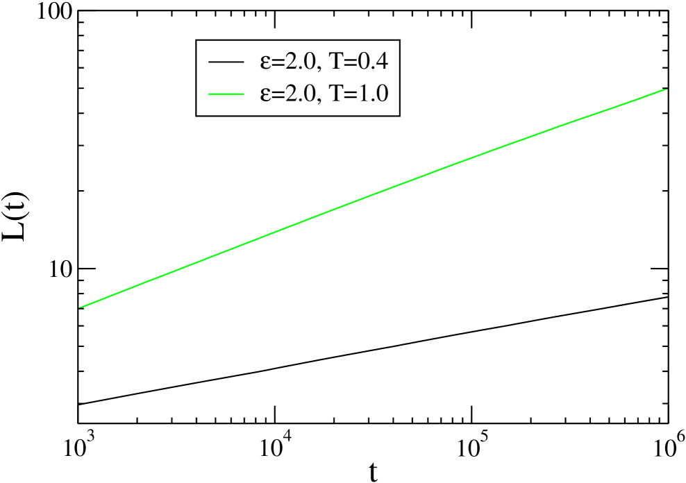
Figure 1: Log-log plot of the dynamical correlation length $L(t)$ as a function of time $t$ for the strongest disorder $\varepsilon=2.0$, with $T=0.4$ and $T=1.0$. Clear deviations from a simple power law are observed for larger times.

As an example we show in Figure 1 the time evolution of $L(t)$ for $\varepsilon=2.0$ and two different temperatures. In both cases clear deviations from an algebraic growth are observed at later times. Our simulations do not allow us to access the asymptotic long time regime, so that we can not affirm that this regime is characterized by a logarithmic growth. Comparing with the corresponding lengths obtained in the random-site Ising model Par10 , we note that the deviations in Figure 1 are much less pronounced than those observed for the random-site model. Another way of stating this is that the transient, algebraic-like regime extends to longer times in the random-bond case. Obviously, no theoretical approach is known that allows us to give an analytical expression for the observed crossover of $L(t)$. For that reason we are going to use the numerically determined quantity in the following analysis of the two-times correlation function.

3.2 Two-time autocorrelation function

In this paper we probe aging scaling exclusively through the behavior of the spin-spin correlation function

$$C(t,s;r)=\frac{1}{N^{2}}\sum\limits_{\textbf{x}}\overline{\langle S_{\textbf{x}+\textbf{r}}(t)S_{\textbf{x}}(s)\rangle}$$ (5)

If $r=0$, then we are dealing with the autocorrelation function $C(t,s)=C(t,s;r=0)$.

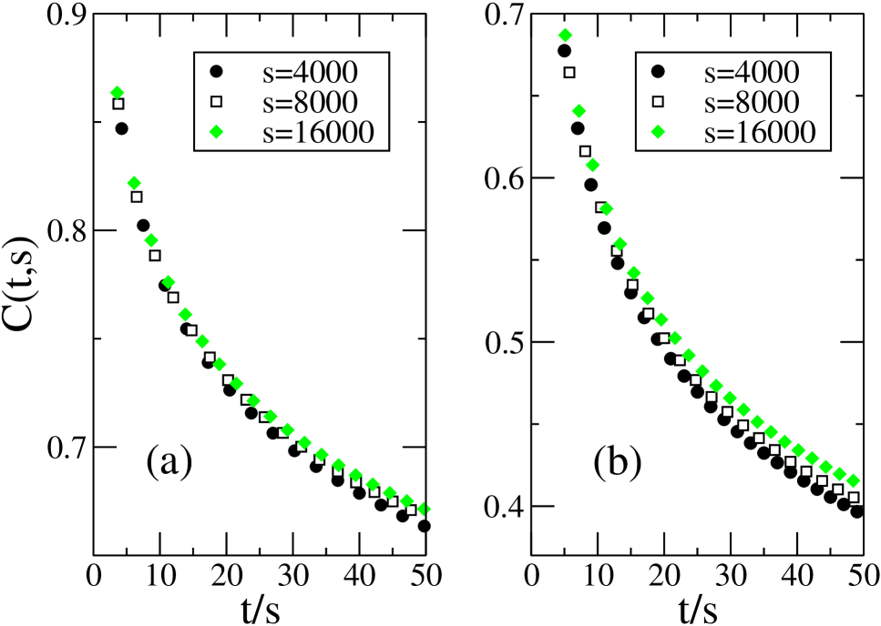
Figure 2: Autocorrelation function versus $t/s$ for $\varepsilon=2.0$, with (a) $T=0.4$ and (b) $T=1.0$. The data do not fall on a common master curve. Approximate scaling can only be obtained for unphysical, negative values of the exponent $b$, see equation (6). Here and in the following error bars are much smaller than the sizes of the symbols.

If one assumes an algebraic growth law, $L(t)\sim t^{1/z}$, then the scaling (1) reduces to

$$C(t,s)=s^{-b}\tilde{f}_{c}(t/s)~{},$$ (6)

where the scaling function $\tilde{f}_{c}(t/s)$ only depends on the ratio $t/s$. However, both for the random-site Pau07 ; Par10 and random-bond Hen06 ; Hen08 models only an extremely poor scaling is obtained when plotting the autocorrelation function versus $t/s$. An approximate scaling can be achieved with some negative exponent $b$, but this is unphysical Hen06 ; Pau07 . In Figure 2 we show the poor scaling for $\varepsilon=2.0$ for two different temperatures. Deviations are less pronounced at lower temperature, as here the transient algebraic growth persists for longer times, see Figure 1.

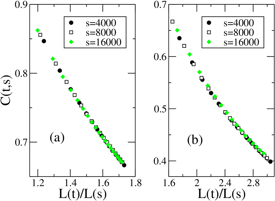
Figure 3: Autocorrelation function versus $L(t)/L(s)$ for $\varepsilon=2.0$, with (a) $T=0.4$ and (b) $T=1.0$. The time-dependent lengths $L$ have been determined numerically, see Figure 1. The data now collapse on a common master curve, in agreement with the simple aging scaling (1).

As all this is similar to what is observed in the random-site model Par10 , we proceed in the same way as in our previus study. Instead of assuming a certain analytical form for $L(t)$ (which we could not derive anyhow, due to the crossover between the two regimes), we use the numerically determined values for $L(t)$ in order to check for scaling. The results of this procedure are shown in Figure 3 for the same two cases as those shown in Figure 2. In all studied cases, a perfect data collapse is observed when plotting $C$ as a function of $L(t)/L(s)$. It follows that the simple aging scaling (1), with $B=0$, also prevails in the random-bond disordered ferromagnet when using the correct growth law $L(t)$.

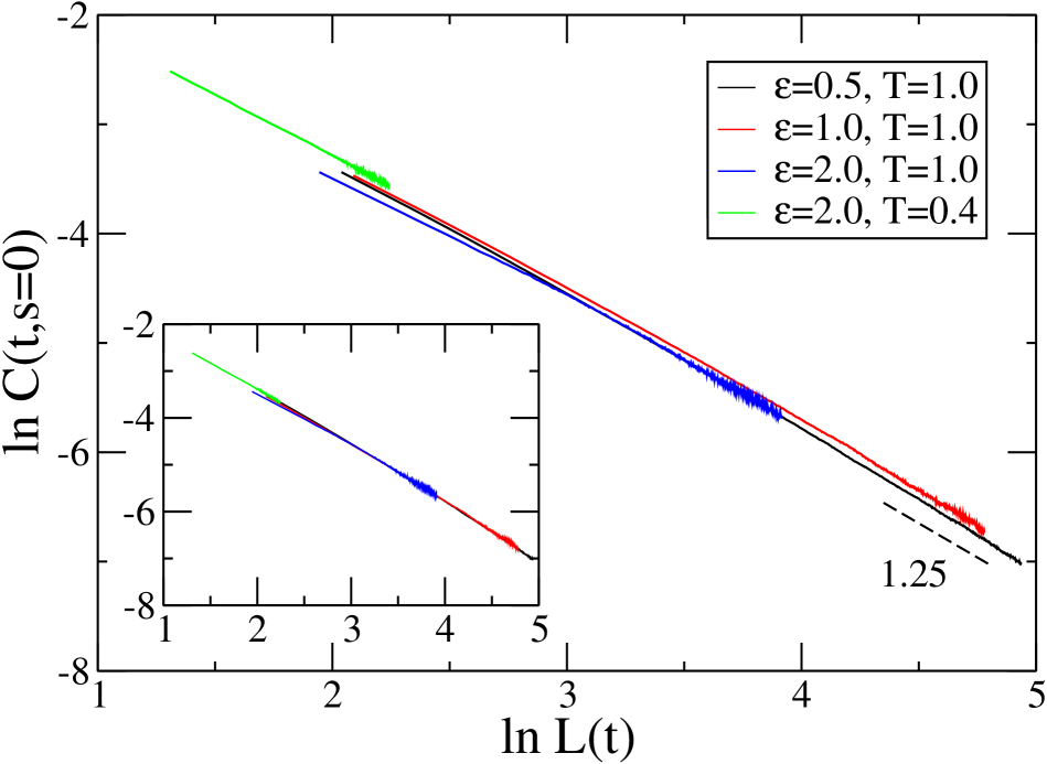
Figure 4: Log-log plot of $C(t,s=0)$ vs. $L(t)$ for four different cases. The dashed line indicates the slope 1.25 measured in the perfect Ising model. As shown in the inset, shifting the different curves vertically makes them overlap, giving some indication that the same slope could emerge for $L(t)\gg 1$ in all cases.

In Cor11a Corberi et al. showed that for the random-bond model the autocorrelations for different values of $\varepsilon$ and different temperatures $T$ are in general not identical when plotted against $L(t)/L(s)$ (see also Hen08 ). Instead, a partial collapse is noted, as data with the same ratio $\varepsilon/T$ fall on a common master curve Hen08 ; Cor11a . All this points to the fact that even as superuniversality is not fully realized (for this the autocorrelation should only depend on $L(t)/L(s)$, irrespective of the values of $\varepsilon$ and $T$), there is still a remarkable degree of universality encountered in the disordered ferromagnets.

Another interesting aspect is revealed in Figure 4 where we plot $C(t,s=0)$ as a function of $L(t)$ for four different cases. From the simple scaling picture we expect that for $L(t)\gg 1$ the autocorrelation varies with $L(t)$ in the form of a power-law Hen10 :

$$C(t,0)\sim\left(L(t)\right)^{-\lambda_{C}}$$ (7)

with the autocorrelation exponent $\lambda_{C}$. For the perfect Ising model, different studies have measured this exponent, yielding the value $\lambda_{C}\approx 1.25$ in two dimensions Fis88 ; Hum91 ; Liu91 ; Lor07 . In Figure 4 we show $C(t,s=0)$ as a function of $L(t)$ for the different disorder distributions and temperatures. Focusing first on the two cases with $\varepsilon=0.5$ and 1, we note that in the log-log plot the corresponding autocorrelation functions are given by straight lines for the larger values of $L$. For the slopes we obtain 1.25(2), i.e. the same value as for the perfect Ising model. For the two cases with $\varepsilon=2$, we are not yet completely in the regime of power-law decay (this is especially true for $T=0.4$ for which only very small values of $L(t)$ are accessible). Still, shifting the curves vertically such that they overlap, see the inset, we see that the two $\varepsilon=2$ curves in fact closely follow the curves for $\varepsilon=0.5$ and 1. This is at least compatible with a common exponent $\lambda_{C}\approx 1.25$ irrespective of disorder, even though we are not able to access the algebraic regime in all cases.

3.3 The space-time correlation function

In an earlier study of the two-times space-time correlation function Hen08 of the random-bond model, intriguing and yet unexplained results were obtained. On the one hand, looking at $C(t,s;r)$ as a function of $r/L(s)$ for $t/s$ fixed, it was found that the scaling functions for various values of $\varepsilon$ and various temperatures are identical to that of the pure model, as would be expected if superuniversality holds, provided the following two conditions are fulfilled: (1) $r/L(s)$ is not too small, $r/L(t)\gtrsim 0.5$, and (2) $\varepsilon$ is stricly less than 2. The first condition of course agrees with the observation that superuniversality is absent for the autocorrelation Cor11a , which corresponds to $r=0$. A possible explanation for the second condition could be that much longer times $t$ (much larger $L(t)$) are needed in order to see the crossover to the scaling function of the pure model for the limiting case where some couplings are very small or even zero.

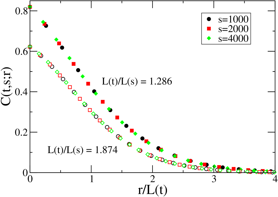
Figure 5: Space-time correlation function as a function of $r/L(t)$ for two different ratios $L(t)/L(s)=1.286$ (filled symbols) and 1.874 (open symbols). The data obtained for different waiting times $s$ fall on a common curve.

All these results have been analyzed in Hen08 under the assumption of an algebraic growth law. We therefore present in the following results for the space-time correlation function $C(t,s;r)$ where the numerically determined length $L(t)$ is used.

We first verify in Figure 5 for the case $\varepsilon=2.0$ and $T=0.4$ that $C(t,s;r)=C(L(t)/L(s),r/L(t))$, i.e. the space time correlation only depends on $L(t)/L(s)$ and $r/L(t)$. Fixing $L(t)/L(s)$ we see that data obtained for different waiting times $s$ indeed fall on a common scaling curve when plotted against $r/L(t)$.

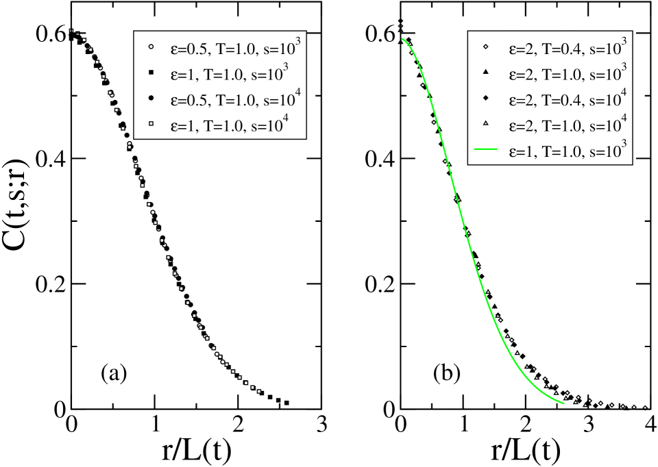
Figure 6: Space-time correlation function as a function of $r/L(t)$ for the fixed value $L(t)/L(s)=1.9$. (a) Comparison of the scaling functions obtained for $\varepsilon=0.5$ and 1, with $T=1$ and two different waiting times. (b) The scaling function obtained for $\varepsilon=2$ differs from the scaling function (green line) shown in (a).

The scaling functions obtained for different disorder distributions and different temperatures are compared in Figure 6. Panel (a) shows for $\varepsilon=0.5$ and 1, both at temperature $T=1$, and different waiting times that the data obtained for the space-time correlation at fixed $L(t)/L(s)$ collapse. A close inspection shows that the resulting scaling function agrees with that of the perfect Ising model. Noting that the ratio $\varepsilon/T$ is not the same for the two cases shown in panel (a), the observation of a data collapse for our space-time quantity goes beyond the partial collapse discussed in Cor11a where autocorrelations with the same value of $\varepsilon/T$ are found to agree. In agreement with Cor11a we observe notable deviations from a common curve also for the space-time correlation when $r/L(t)$ is small. As shown in panel (b) data obtained for $\varepsilon=2$ and different temperatures show also rather good collapse for a fixed value of $L(t)/L(s)$. However the resulting scaling function still differs from that obtained for smaller values of $\varepsilon$. Using the numerically determined length $L(t)$ does therefore not allow to resolve this issue initially raised in Hen08 .

4 The three-dimensional Ising spin glass

4.1 Dynamical correlation length

For the Edwards-Anderson spin glass we need to proceed slightly differently in order to obtain the dynamical correlation length. We consider two replicas $\left\{S_{\textbf{x}}^{(\alpha)}(t)\right\}$ and $\left\{S_{\textbf{x}}^{(\beta)}(t)\right\}$ with the same set of bonds and consider the overlap field

$$q_{\textbf{x}}(t)=S_{\textbf{x}}^{(\alpha)}(t)S_{\textbf{x}}^{(\beta)}(t)~{}.$$ (8)

The quantity of interest is then the one-time space-time correlator (we use the same notation as for the random-bond model discussed in the previous section, even though this is a different quantity)

$$G(t;r)=\frac{1}{N^{3}}\sum_{\textbf{x}}\overline{\langle q_{\textbf{x}}(t)q_{\textbf{x+r}}(t)\rangle}$$ (9)

where $N^{3}$ is the total number of sites in our system. One additional complication comes from the fact that the decay of $G(r;t)$ is not given by a simple exponential, but instead one has that

$$G(t;r)\sim\frac{1}{r^{a}}F\left(\frac{\textbf{r}}{L(t)}\right)$$ (10)

where $a\approx 0.4$ for the three-dimensional case Mar01 , whereas $F(x)=\exp[-x^{\beta}]$ with $\beta\sim 1.5$ Jim05 . Using the method of integral estimators proposed in Bel09 , we note that the dynamical correlation length is proportional to the following ratio of integrals:

$$L(t)\propto\frac{I_{2}(t)}{I_{1}(t)}~{},$$ (11)

where

$$I_{k}(t)\equiv\int^{N/2}_{0}\textrm{d}r\,r^{k}G(t;r)~{}.$$ (12)

We can use $N/2$ as the upper integration boundary as we make sure that $N\gg L(t)$.

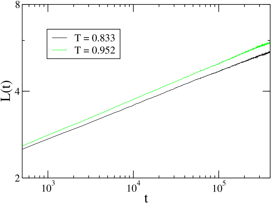
Figure 7: Dynamical correlation length versus time for the three-dimensional Edwards-Anderson spin glass, as obtained from equation (11). For both temperatures, no strong deviations from an algebraic growth are observed during our simulations.

In Figure 7 we show the dynamical length that we obtain from equation (11) for the two temperatures $T=0.833$ and $T=0.952$. We note that after 400000 MCS the dynamical length is still less than 6 lattice constants, which reveals the expected very slow dynamics. Also, only very minor deviations from a straight line are observed in this double logarithmic plot.

4.2 Two-time autocorrelation function

The fact that for our simulation times the length $L(t)$ does not display obvious deviations from an algebraic growth already indicates that two-times quantities should rather well fulfill the equation (6) obtained under the assumption that $L\sim t^{1/z}$. This is indeed the case, as shown in Figure 8 for the two-times spin-spin autocorrelation function $C(t,s)$ at temperature $T=0.833$. We also note that for the Ising spin glass the exponent $B$ is not zero, as already remarked in earlier studies Kis96 . However, a closer inspection reveals that there are systematic deviations, both for small and for large values of $t/s$. Indeed, for small values of $t/s$ the data obtained for the smallest waiting time has the highest value for the autocorrelation function, whereas for large values of $t/s$ the smallest waiting time yields the lowest value (see inset).

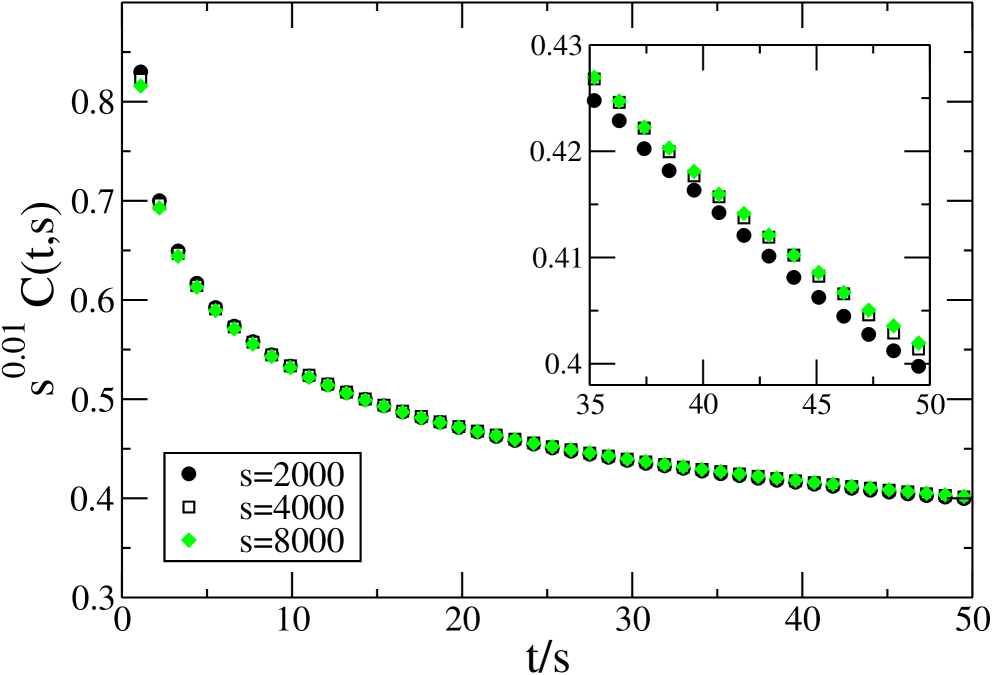
Figure 8: Autocorrelation as a function of $t/s$ for the three-dimensional Ising spin glass at temperature $T=0.833$. Deviations from the scaling (6) are observed both for small and for large value of $t/s$, see inset.

We therefore reanalyze the data by using the numerically determined length $L(t)$ of Figure 7 instead of simply assuming a perfect power-law increase. For both studied temperatures no systematic deviations are observed any more when plotting $C(t,s)$ as a function of $L(t)/L(s)$. We therefore conclude that also for the Ising spin glass the aging scaling (1) with the correct $L(t)$ prevails. Whereas this is the same conclusion as for the disordered ferromagnets, we point out that there is a notable difference between the disordered ferromagnets and the frustrated spin glass: for the former we have that $B=0$, whereas for the latter the exponent $B$ is different from zero and depends on the temperature, see Figure 9.

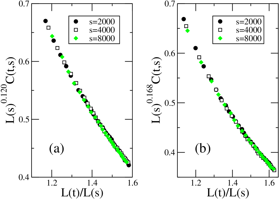
Figure 9: Autocorrelation as a function of $L(t)/L(s)$ for the three-dimensional Ising spin glass at temperature (a) $T=0.833$ and (b) $T=0.952$. No systematic deviations from the scaling (1) are observed. Note that the scaling exponent $B$ is different form zero and that its value depends on the temperature.

5 Discussion and conclusion

Phase ordering in disordered systems, both with or without frustration, still poses many challenges. Due to the very slow dynamics, it is usually not possible to enter the asymptotic regime. Instead, most studies have been done in the initial, transient regime where the typical length in the system increases approximately like a power-law of time. Still, an increasing number of studies noticed deviations from the simple algebraic growth at later time, pointing to a crossover from the algebraic-like regime to the true asymptotic regime.

In the past when studying phase ordering in disordered systems, one usually assumed an algebraic growth law, yielding a scaling behavior like that given in equation (6). However, recent studies have shown that disordered ferromagnets do not display a good scaling under the assumption of a power-law growth, $L(t)\sim t^{1/z}$, of the dynamical correlation length $L(t)$ Hen06 ; Pau07 ; Hen08 . In Par10 we studied aging in the random-site Ising model where we did not make any assumption on the functional form of $L(t)$ but instead used the numerically determined length $L(t)$ in the analysis. As a result we obtained that two-times quantities fulfilled the simple aging scaling (1), irrespective of the degree of dilution.

In this paper we have applied the same analysis to another disordered ferromagnet, the random-bond ising model in two dimensions, as well as to the three-dimensional Edwards-Anderson spin glass. For the random-bond model notable deviations from simple scaling can be observed when using $t/s$ as scaling variable, similar, but less pronounced, to what is encountered in the random-site case. We find that for both models the simple aging scaling (1) is recovered when using as scaling variable $L(t)/L(s)$ with the numerically determined length $L$. Thus even small deviations from an algebraic growth can have a large impact on aging scaling and need to be taken into account in a correct description. However, as we do not have currently analytical expressions of $L(t)$ in disordered systems with a crossover from an algebraic to a slower (logarithmic?) growth, we are bound to use the numerically determined function $L(t)$.

We also briefly discussed some issues related to the concept of superuniversality. Whereas superuniversality, i.e. an independence of scaling functions on disorder when using $L(t)$ in time-dependent quantities, in the strict sense is surely not realized, there is still a remarkable degree of universality that can be encountered in disordered ferromagnets undergoing phase ordering. This universality strongly shows up in the two-times space-time correlation function for not too short distances, as scaling functions are found to be independent of disorder and of temperature in that regime. The only exception is encountered for $\varepsilon=2$, i.e. the strongest disorder where very weak bonds are present. More extensive studies will be needed in order to fully understand this remarkable behavior of space-time quantities in the aging regime.

References

- (1) A. J. Bray, Adv. Phys. 43, 357 (1994).
- (2) S. Puri, in Kinetics of Phase Transitions, edited by S. Puri and V. Wadhawan (CRC Press, Boca Raton, FL, 2009) 1.
- (3) F. Corberi, L. F. Cugliandolo, and H. Yoshino, in Dynamical Heterogeneities in Glasses, Colloids, and Granular Media, edited by L. Berthier, G. Biroli, J.-P. Bouchaud, L. Cipelleti, and W. Van Saarloos (Oxford University Press, Oxford, 2011).
- (4) M. Henkel and M. Pleimling, Non-Equilibrium Phase Transitions Vol. 2: Ageing and Dynamical Scaling Far from Equilibrium (Springer, Heildeberg, 2010).
- (5) D. S. Fisher and D. A. Huse, Phys. Rev. B 38, 373 (1988).
- (6) K. Humayun and A. J. Bray, J. Phys. A: Math. Gen. 24, 1915 (1991).
- (7) F. Liu and G. F. Mazenko, Phys. Rev. B 44, 9185 (1991).
- (8) F. Corberi. A. Coniglio, and M. Zannetti, Phys. Rev. E 51, 5469 (1995).
- (9) C. Godrèche and J.-M. Luck, J. Phys. A: Math. Gen. 33, 1151 (2000).
- (10) C. Godrèche and J.-M. Luck, J. Phys. Cond. Matt. 33, 9141 (2000).
- (11) E. Lippiello and M. Zannetti, Phys. Rev. E 61, 3369 (2000).
- (12) M. Henkel, M. Pleimling, C. Godrèche, and J.-M. Luck, Phys. Rev. Lett. 87, 265701 (2001).
- (13) F. Corberi, E. Lippiello, and M. Zannetti, Phys. Rev. E 68, 046131 (2003).
- (14) M. Henkel and M. Pleimling, Phys. Rev. E 68, 065101(R) (2003).
- (15) M. Henkel, M. Paeßens, and M. Pleimling, Europhys. Lett. 62, 644 (2003).
- (16) M. Henkel, M. Paeßens, and M. Pleimling, Phys. Rev. E 69, 056109 (2004).
- (17) M. Henkel, A. Picone, and M. Pleimling, Europhys. Lett. 68, 191 (2004).
- (18) S. Abriet and D. Karevski, Eur. Phys. J. B 36, 47 (2004).
- (19) S. Abriet and D. Karevski, Eur. Phys. J. B 41, 79 (2004).
- (20) E. Lorenz and W. Janke, Europhys. Lett. 77, 10003 (2007).
- (21) F. Corberi and L. F. Cugliandolo, J. Stat. Mech., P05010 (2009).
- (22) T. Mukherjee, M. Pleimling, and Ch. Binek, Phys. Rev. B 82, 134425 (2010).
- (23) E. Vincent, in Ageing and the Glass Transition, edited by M. Henkel, M. Pleimling, and R. Sanctuary (Springer, Heidelberg, 2007).
- (24) N. Kawashima and H. Rieger, in Frustrated Magnetic Systems, edited by H. Diep (World Scientific, Singapour, 2004).
- (25) J. Kisker, L. Santen, M. Schrechenberg, and H. Rieger, Phys. Rev. B 53, 6418 (1996).
- (26) E. Marinari, G. Parisi, F. Ritort, and J. J. Ruiz-Lorenzo, Phys. Rev. Lett. 76, 843 (1996).
- (27) G. Parisi, F. Ricci-Tersenghi, and J. J. Ruiz-Lorenzo, J. Phys. A 29, 7943 (1996).
- (28) H. Yoshino, K. Hukushima, and H. Takayama, Phys. Rev. B 66, 064431 (2002).
- (29) L. Berthier and J.-P. Bouchaud, Phys. Rev. B 66, 054404 (2002).
- (30) F. Belleti et al., J. Stat. Phys. 135, 1121 (2009).
- (31) R. Paul, S. Puri, and H. Rieger, Europhys. Lett. 68, 881 (2004).
- (32) R. Paul, S. Puri, and H. Rieger, Phys. Rev. E 71, 061109 (2005).
- (33) M. Henkel and M. Pleimling, Europhys. Lett. 76, 561 (2006).
- (34) R. Paul, G. Schehr, and H. Rieger, Phys. Rev. E 75, 030104(R) (2007).
- (35) C. Aron, C. Chamon, L. F. Cugliandolo, and M. Picco, J. Stat. Mech., P05016 (2008).
- (36) M. Henkel and M. Pleimling, Phys. Rev. B 78, 224419 (2008).
- (37) M. P. O. Loureiro, J. J. Arenzon, L. F. Cugliandolo, and A. Sicilia, Phys. Rev. E 81, 021129 (2010).
- (38) H. Park and M. Pleimling, Phys. Rev. B 82, 144406 (2010).
- (39) F. Corberi, E. Lippielli, A. Mukherjee, S. Puri, and M. Zannetti, J. Stat. Mech., P03016 (2011).
- (40) F. Corberi, E. Lippielli, A. Mukherjee, S. Puri, and M. Zannetti, Phys. Rev. E 85, 021141 (2012).
- (41) A. Kolton, A. Rosso, and T. Giamarchi, Phys. Rev. Lett. 95, 180604 (2005).
- (42) J. D. Noh and H. Park, Phys. Rev. E 80, 040102(R) (2009).
- (43) J. L. Iguain, S. Bustingorry, A. B. Kolton, and L. F. Cugliandolo, Phys. Rev. B 80, 094201 (2009).
- (44) C. Monthus and T. Garel, J. Stat. Mech., P12017 (2009).
- (45) M. Nicodemi and H. J. Jensen, Phys. Rev. B 65, 144517 (2002).
- (46) C. J. Olson, C. Reichhardt, R. T. Scalettar, G. T. Zimanyi, and N. Grønbach-Jensen, Phys. Rev. B 67, 184523 (2003).
- (47) G. Schehr and P. Le Doussal, Phys. Rev. Lett. 93, 217201 (2004).
- (48) S. Bustingorry, L. F. Cugliandolo, and D. Dominguez, Phys. Rev. Lett. 96, 027001 (2006).
- (49) S. Bustingorry, L. F. Cugliandolo, and D. Dominguez, Phys. Rev. B 75, 024506 (2007).
- (50) X. Du, G. Li, E.Y. Andrei, M. Greenblatt, and P. Shuk, Nature Physics 3, 111 (2007).
- (51) M. Pleimling and U. C. Täuber, Phys. Rev. B 84, 174509 (2011).
- (52) D. A. Huse and C. L. Henley, Phys. Rev. Lett. 54, 2708 (1985).
- (53) A. J. Bray and K. Humayun, J. Phys. A 24, L1185 (1991).
- (54) S. Puri, D. Chowdhuri, and N. Parekh, J. Phys. A 24, L1087 (1991).
- (55) H. Hayakawa, J. Phys. Soc. Jpn. 60, 2492 (1991).
- (56) T. Iwai and H. Hayakawa, J. Phys. Soc. Jpn. 62, 1583 (1993).
- (57) B. Biswal, S. Puri, and D. Chowdhuri, Physica A 229, 71 (1996).
- (58) H. G. Katzgraber, M. Koerner, and A. P. Young, Phys. Rev. B 73, 224432 (2006).
- (59) E. Marinari and G. Parisi, Phys. Rev. Lett. 86, 3887 (2001).
- (60) S. Jimenez, V. Martin-Mayor, and S. Perez-Gaviro, Phys. Rev. B 72, 054417 (2005).