An optimistic CoGeNT analysis

Abstract

Inspired by a recently proposed model of millicharged atomic dark matter (MADM), we analyze several classes of light dark matter models with respect to CoGeNT modulated and unmodulated data, and constraints from CDMS, XENON10 and XENON100. After removing the surface contaminated events from the original CoGeNT data set, we find an acceptable fit to all these data (but with the modulating part of the signal making a statistically small contribution), using somewhat relaxed assumptions about the response of the null experiments at low recoil energies, and postulating an unknown modulating background in the CoGeNT data at recoil energies above 1.5 keVee. We compare the fits of MADM—an example of inelastic magnetic dark matter—to those of standard elastically and inelastically scattering light WIMPs (eDM and iDM). The iDM model gives the best fit, with MADM close behind. The dark matter interpretation of the DAMA annual modulation cannot be made compatible with these results however. We find that the inclusion of a tidal debris component in the dark matter phase space distribution improves the fits or helps to relieve tension with XENON constraints.

I Introduction

It is an exciting time, albeit puzzling, for direct detection of dark matter. The three experiments DAMA Bernabei:2008yi , CoGeNT Aalseth:2010vx ; Aalseth:2011wp and CRESST Angloher:2011uu see hints of light DM of mass $\sim 10$ GeV and cross section $\sim 10^{-40}$ cm² for scattering on nucleons. Although much effort has been made to determine whether DAMA and CoGeNT best-fit regions (and possibly those of CRESST) can be compatible Fitzpatrick:2010em -Foot:2012rk , it is difficult to find any dark matter model which achieves this quantitatively, and which moreover is consistent with the null results of XENON10 Angle:2011th , XENON100 Aprile:2011hi , CDMS Ahmed:2009zw ; Ahmed:2010wy ; Ahmed:2012vq , and most recently EDELWEISS edelweiss .  It seems unlikely that all of the hints of positive detections can be correct since even nonstandard DM models with many adjustable parameters give a poor fit to the global data Frandsen:2011ts ; Schwetz:2011xm ; Farina:2011pw . Arguably, the best hope for reconciling the positive and negative signals centers around the CoGeNT results, which can be compatible with the lightest and most weakly coupled DM models, hence those having the greatest chance of being marginally compatible with the null results. This is our motivation for focusing the present study on CoGeNT.

Another of the difficulties with CoGeNT is that it presents an annual modulation amplitude that seems to be too large compared to the unmodulated rate unless a nonstandard velocity distribution is invoked for dark matter in the galactic halo Fox:2011px ; McCabe:2011sr ; Arina:2011zh . This problem is only exacerbated by recent results indicating that the earlier published events included contamination from surface events collar . If CoGeNT is indeed seeing dark matter, it is tempting to speculate that there is some contamination of the modulating part of the signal that should be subtracted, to ameliorate this tension. We explore the effect of including such a background, finding that the CoGeNT-allowed regions of parameter space are hardly affected by the modulating part of the data, regardless of any such background, due to their lower statistical significance relative to the time-averaged part of the signal.

Although we also consider standard elastic and inelastic dark matter in the present study, one of our motivations for carrying it out was the proposal of a new class of millicharged atomic dark matter (MADM) models in Cline:2012is (a simpler variant of models previously discussed in refs. Kaplan:2009de ; Kaplan:2011yj ), with emphasis on the special case where the dark “electron” and “proton” constituents have equal masses, $m_{\mathbf{e}}=m_{\mathbf{p}}$. In the ref. Cline:2012is , rough estimates were made as to the parameter values required to explain the CoGeNT observations. Here we better quantify those by direct comparison to the data. We will show that MADM gives an acceptable fit to the data for the dark ${\mathbf{H}}$ atom mass $m_{\mathbf{H}}\sim 10$ GeV, the hyperfine mass splitting $\delta m_{\mathbf{H}}\sim 25$ keV, and the fractional charge of the ${\mathbf{e}}$ and ${\mathbf{p}}$ constituents $\epsilon\sim 0.01$, which controls the scattering cross section. The fit to the CoGeNT data by MADM is better than the one of standard elastic dark matter (eDM), and only slightly worse than that of standard inelastic dark matter (iDM), which requires similar values for the mass and mass splitting.

It is interesting to note that in the special $m_{\mathbf{e}}=m_{\mathbf{p}}$ case of interest, the effective charge of dark atoms is zero even at short wavelengths, due to the cancellation between the charge clouds of the two constituents, and the model becomes an example of magnetic inelastic dark matter Chang:2010en -Weiner:2012cb (this identification has not been previously realized). Magnetically interacting dark matter has recently been promoted as a model that can fit “everything,” all the null and positive direct detection constraints DelNobile:2012tx , including DAMA and CRESST. In the present work, we will not reach such optimistic conclusions, even though we find some room for CoGeNT to be compatible with the Xenon and CDMS constraints, if we exercise a moderate degree of skepticism concerning the claimed sensitivity of the Xenon experiments to low recoil energy events.

We also consider the effect of astrophysical uncertainties, including nonMaxwellian velocity distributions Lisanti:2010qx and contributions from debris flow Lisanti:2011as ; Kuhlen:2012fz . We find quantitative changes to the allowed regions as a result of these variations, and in the case of debris flow, some improvement in the quality of the fits and in the relative size of CoGeNT-allowed versus excluded regions. In the remainder of the paper, we will review the theoretical framework (section II) and our methods of analysis of the various experiments (section III). Results are presented in section IV and conclusions in section V.

II The models and their predictions

We briefly review the MADM model and highlight its differences relative to standard (inelastic) dark matter for direct detection. The MADM model contains a dark “electron” ${\mathbf{e}}$ and “proton” ${\mathbf{p}}$ bound into dark atoms ${\mathbf{H}}$ by a new U(1) gauge force of strength $\alpha^{\prime}$, whose massless vector boson kinetically mixes with the photon, resulting in a small electric charge $\pm\epsilon e$ for the ${\mathbf{e}}$, ${\mathbf{p}}$ constituents. MADM therefore interacts electromagnetically with protons in ordinary nuclei. In the special case where $m_{\mathbf{e}}=m_{\mathbf{p}}$, the electric coupling vanishes in the leading Born approximation and the dominant transition is via the atomic hyperfine interaction. It is inelastic due to the hyperfine splitting $\delta m_{\mathbf{H}}=\frac{8}{3}\alpha^{\prime 4}m_{\mathbf{e}}^{2}m_{\mathbf{p}}^{2}/(m_{\mathbf{e}}+m_{\mathbf{p}})^{3}$ which can naturally be of order 10 keV.

In general, the differential rate of DM scattering on nuclei with nuclear recoil energy $E_{R}$ is given by

$$\frac{\mathrm{d}R}{\mathrm{d}E_{R}}=N_{T}\frac{\rho_{\odot}}{m_{DM}}\int_{v>v_{\rm min}}\mathrm{d}^{\,3}v\,vf(v)\frac{\mathrm{d}\sigma}{\mathrm{d}E_{R}}\ ,$$ (1)

where $N_{T}$ is the number of target nuclei, $\rho_{\odot}\cong 0.43$ GeV/cm³ Salucci:2010qr is the DM density in the solar neighborhood, $m_{DM}$ is the DM mass, $f(v)$ is its velocity distribution (see appendix A for details), and $v_{\rm min}$ is the minimum DM velocity needed to produce the given recoil energy. In terms of the momentum transfer $q=\sqrt{2m_{N}E_{R}}$ for nuclear mass $m_{N}$ and DM-nucleus reduced mass $\mu$, it is $v_{\rm min}=q/(2\mu)+\delta m/q$ for inelastic DM with mass splitting $\delta m$. The differential cross section for DM of velocity $v$ scattering on nuclei can be expressed as

$$\frac{\mathrm{d}\sigma}{\mathrm{d}E_{R}}=\frac{m_{N}\sigma_{p}}{2v^{2}\mu_{n}^{2}}{\left[Z+{f_{n}\over f_{p}}(A-Z)\right]^{2}}F_{N}^{2}(q)\,F_{DM}^{2}(q,v)$$ (2)

where $\sigma_{p}$ is the cross section for DM scattering on protons at threshold, $\mu_{n}$ the DM-nucleon reduced mass, $F_{N}$ the Helm nuclear form factor Lewin:1995rx , and $F_{DM}$ the DM form factor. For generic DM, $f_{n}/f_{p}=F_{DM}=1$, whereas for MADM, $f_{n}=0$ and $F_{DM}\sim(v^{2}-v_{\rm min}^{2})/q^{2}$.

In the MADM model, the differential detection rate for spin-independent scattering can be expressed as

$${dR\over dE_{R}}={\pi N_{T}\rho_{\mathbf{H}}\over m_{\mathbf{H}}\,E_{R}}\left({4\epsilon\alpha ZF_{H}\over m_{\mathbf{H}}}\right)^{2}\,I(v_{\rm min},\vec{v}_{e})$$ (3)

where the velocity integral is given by

$$I(v_{\rm min},\vec{v}_{e})=\int_{v_{\rm min}}{d^{\,3}v\over v}\left(v^{2}-v_{\rm min}^{2}\right)f(\vec{v}+\vec{v}_{e})$$ (4)

(see appendix B for details). Because of the $F_{DM}$ form factor, $\sigma_{p}$ cannot be defined in the usual way as the cross section at threshold, but if desired, one can define an effective $\sigma_{p}$ by inserting characteristic values $v_{0}$, $q_{0}$ of the DM velocity and momentum transfer,

$$\sigma_{p}=\frac{64\pi\epsilon^{2}\alpha^{2}\mu_{n}^{2}v_{0}^{2}}{m_{\mathbf{H}}^{2}q_{0}^{2}}\ ,$$ (5)

for example $q_{0}=25$ MeV (appropriate for scattering on germanium at $E_{R}=5$ keV), $v_{0}=220$ km/s. The form factor has compensating such terms,

$$F_{DM}^{2}(q,v)=\frac{q_{0}^{2}}{q^{2}}\frac{\left(v^{2}-v_{\rm min}^{2}\right)}{v_{0}^{2}}$$ (6)

so that the rate is independent of $v_{0}$, $q_{0}$.

In addition, there is a spin-dependent dipole-dipole scattering interaction that was neglected in Cline:2012is . This neglect turns out to be justified for scattering on germanium and xenon, but not for iodine and especially sodium. In appendix B we give details of the dipole-dipole scattering rate, and estimates that establish the previous statement. Accordingly we will neglect spin-dependent interactions in the remainder of this paper, except for our brief study of the prospects for accommodating the DAMA annual modulation in our global fit.

In the following, we will be interested not only in MADM but also in generic DM models where $F_{DM}=1$, which can be elastic ($v_{\rm min}=q/(2\mu)$) or inelastic ($v_{\rm min}=q/(2\mu)+\delta m/q$). We note that MADM differs from the generic inelastic DM model (iDM) not only because of the form factor (6), but also because of its mild isospin violation, $f_{n}=0$. In this work we do not investigate models with arbitrary isospin violation, such as the case of $f_{n}/f_{p}=-0.7$ that significantly weakens the sensitivity of xenon-based experiments Chang:2010yk ; Feng:2011vu ; An:2011ck ; Cline:2011zr ; Frandsen:2011ts ; Schwetz:2011xm ; Farina:2011pw . However we will consider both the isospin conserving eDM and iDM models, and the special case in which $f_{n}=0$. The latter occurs naturally when DM interactions are mediated by a U(1) gauge boson that kinetically mixes with the photon.

III Methodology

In this section we describe the computation of $\chi^{2}$ for the CoGeNT modulated and unmodulated data, DAMA modulations, and the exclusion contours coming from XENON100, XENON10 and CDMS-Ge (CDMS-Si gives weaker limits for the models of interest). Some of this is standard, following the same procedures as the relevant experimental collaborations themselves. In the case of CoGeNT, we suggest an additional background to be subtracted (over and above the surface contamination events discussed in collar ), namely an unspecified modulating background that we take to be independent of energy, to fit away the modulation of the CoGeNT high-energy bin 1.5–3.1 keVee. However in the end we will find that the experimental errors on the modulating part of the signal are too large for any of these details to matter for the combined fit to the modulating and unmodulated data.

III.1 CoGeNT unmodulated signal

We start by fitting to the CoGeNT unmodulated signal by itself, since this has higher statistical significance than the annual modulation signal. We analyzed the public release data cogentdata provided by the CoGeNT collaboration by reweighting each event using the detector efficiency $f_{\text{eff}}(E)$ Aalseth:2011wp . To remove the known background due to cosmogenic L-shell electron capture events in the region of interest, we used the fitting parameters from the K-shell peaks provided by CoGeNT cogentdata and the ratio between L-shell and K-shell decays Bahcall:1963zza (see e.g. also Farina:2011pw ; Fox:2011px for the parameters of the cosmogenic backgrounds). To relate the observed ionization energy to the inferred nuclear recoil energy, we take the same quenching factor as used by CoGeNT cogentdata , $E/$keVee $=Q(E_{R}/$keVnr$)^{p}$, with $Q=0.2$ and $p=1.12$.

Subsequent to their published results, CoGeNT reported a new estimate of the surface event contamination near the energy threshold collar . We apply the central curve of the estimated surface event correction factor on p. 14 of ref. collar to the energy spectrum after removing the cosmogenic background. A constant background of 2.685 cpd/keVee, taken as the average of the event rate between 2 keVee and 3 keVee, is further subtracted in order to remove the events above $E=1.5$ keVee, whose energy dependence is approximately constant. This is motivated by the fact that light DM models that account for the large excess at lower energies predict essentially no events in this higher energy range. For the errors on each bin, we consider the statistical errors based on the original events in the bin before efficiency correction and background subtraction, and also the uncertainties in the parameters of the cosmogenic background.

In fig. 1 we display the data with the cosmogenic background, surface events contamination, and the constant background subtracted, along with the prediction of the MADM model with parameter values $m_{\mathbf{H}}=9.9$ GeV, $\delta_{\mathbf{H}}=24.7$ keV, $\epsilon=0.029$. Below we will show that this model (which we refer to as our benchmark) corresponds to the best fit parameters and is marginally allowed by XENON constraints, as we will determine them.

To accurately predict the theoretical DM contribution, one should take into account that the 442 day period of CoGeNT data-taking is not an integer multiple of a year, as well as account for inspection and power outage days of the CoGeNT operation, and average the modulated rate over the actual period rather than assuming the mean value of the earth’s velocity relative to the DM halo rest frame. We find that the latter makes a $-1.7$% correction in the predicted rate, too small to be of interest given the current experimental uncertainties.

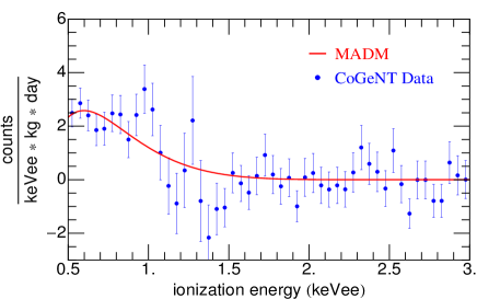
Figure 1: CoGeNT energy spectrum (subtracting cosmogenic background, surface contamination, and constant background), and the prediction from the MADM model, ($m_{\mathbf{H}}$, $\delta_{\mathbf{H}}$, $\epsilon$)=(9.9 GeV, 24.7 keV, 0.029).

III.2 CoGeNT annual modulation

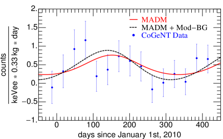
Figure 2: CoGeNT data and MADM (the same model as in Fig.(1) prediction for modulation in the low-energy 0.5-1.5 keVee bin. Here we also consider the possibility of including a modulation background (dashed line) on top of the MADM signal in order to explain the CoGeNT modulation events in the high energy bins. The modulation background used here is $D\sin((2\pi/\text{year})(t-t_{0}))$ where $D=-0.487$ cpd/kg/keVee and $t_{0}=199$ d. As shown in the figure, the CoGeNT modulation amplitudes are larger than MADM predictions.

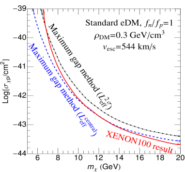
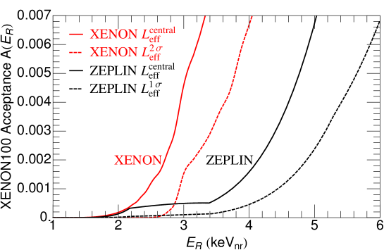
Figure 3: (a) Left: comparison of 90% c.l. limits on elastic DM cross section derived by XENON100 Aprile:2011hi using profile likelihood method (solid, red curve) and by us using maximum gap method with central value (dashed, blue curve) and $2\sigma$ lower limit (dot-dashed, black curve) of the XENON100 relative scintillation efficiency ${\cal L}_{\rm eff}$. (b) Right: XENON100 acceptance curves $A(E_{R})$ for the central values (solid lines) and $2\sigma$ or $1\sigma$ lower limits (dashed lines) of ${\cal L}_{\rm eff}$, taken from ref. Aprile:2011hi (left curves) and Horn:2011wz (right curves). The DM mass is taken to be 10 GeV for the choice of cut acceptance.

We analyzed the modulated data obtained from the CoGeNT collaboration, following ref. Fox:2011px by grouping the events into a low-energy bin with $E<1.5$ keVee and a high-energy bin between $1.5$ and $3.1$ keVee. To determine the modulation spectrum, we model the cosmogenic background by taking into account the outage days. We also remove the constant background and the estimated surface contaminated events collar assuming that they are unmodulated in time. This is supported by the fact that the surface events originally rejected by the CoGeNT analysis of ref. Aalseth:2011wp do not show any sign of modulation. Based on the fit to the unmodulated data, where no dark matter events were found to occur above 1.5 keVee, we consider the modulating signal in the high-energy bin to be due to an unspecified background. To model it using the smallest number of parameters, we take this extra background to be independent of energy, having a rate of the form

$${D\sin(\omega(t-t_{0}))}$$ (7)

Assuming that $\omega=2\pi$ y^-1 so that only $D$ and the phase $t_{0}$ are free parameters, we find that the best fit values are $D=-0.487$ cpd/kg/keVee and $t_{0}=199$ d. It will be seen that these values do not change very much when we allow them vary in the minimization of the total $\chi^{2}$ for all the CoGeNT data. The energy dependence of this hypothetical background is unknown, so we considered the two cases where it either reduces only the signal in the high-energy bin, or that in both. We did not see significant differences between the two possibilities in the final results.

In any case, one needs to separate the data into an unmodulated part (which has already been considered above) and the modulating component whose contribution to $\chi^{2}$ is computed separately from that of the unmodulated signal. We compared several different ways of doing this: fitting the time dependence in a given bin to a constant plus sinusoidal term; splitting the data into its time-averaged value plus fluctuations; or defining the time-dependent part by subtracting the time average only over consecutive 365 day periods rather than 442 days (which should be more correct). However, the data are not yet at the level of precision where these distinctions are important. We find that the time-averaged part of the rate in the low-energy bin is $2.47\pm 0.1$ cpd/keVee (corresponding to the range $\delta\chi^{2}=1)$.

The raw CoGeNT modulation data from the low-energy bin are plotted in fig. 2, along with the MADM prediction plus modulating background (7) for the same model parameter values as used in fig. 1. Although the amplitude of the theoretical prediction looks small compared to the central values of the data, the experimental error bars are large, and so the contribution to the total $\chi^{2}$ from this discrepancy is relatively small. For the benchmark model, ($m_{\mathbf{H}}$, $\delta_{\mathbf{H}}$, $\epsilon$)=(9.9 GeV, 24.7 keV, 0.029), removing the expected DM contribution from the modulation signal in the low-energy bin (0.5-1.5) keVee (i.e., keeping only the modulating background (7) as signal in this energy range), corresponds to a reduction in the total CoGeNT $\Delta\chi^{2}$ of only $\sim 0.5$.

To display the regions of parameter space preferred by the data (see section IV), we use the $\Delta\chi^{2}=3.53,\ 8.03,\ 14.2$ contours, corresponding to confidence intervals of 68.3%, 95.5%, and 99.7%, appropriate for fitting three model parameters ($m_{\mathbf{H}}$, $\delta_{\mathbf{H}}$, $\epsilon$).

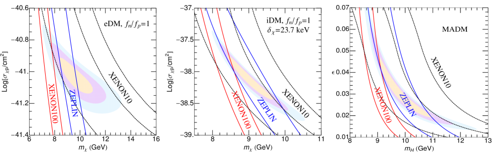
Figure 4: Solid curves: limits from XENON100 assuming the the central and 2$\sigma$ lower limits of the XENON100 ${\cal L}_{\rm eff}$ (leftmost, red lines) and central and 1$\sigma$ lower limit of the ZEPLIN-III ${\cal L}_{\rm eff}$ (rightmost, blue lines). Dashed curves (black): limits from XENON10 assuming the three possible electron yields versus energy shown in fig. 5. The shaded areas are the CoGeNT best-fit regions for eDM (left graph) iDM (central graph) and MADM (right graph) models, discussed in section IV.

III.3 XENON100

The XENON100 collaboration Aprile:2011hi observes 3 events at nuclear recoil energies of 12.1, 30.2 and 34.6 keV respectively, all of which are too high to be directly accounted for by our best-fit models. We compute the number of events above the XENON100 low-energy threshold $8.4$ keVnr using Poisson fluctuations Felixthesis : $N=\int dE_{R}\,dR/dE_{R}\,A(E_{R})$ times the exposure $100.9$ kg $\times\ 48$ d. The acceptance function $A(E_{R})$ depends upon data quality cuts and S2/S1 energy resolution discrimination cuts which we take from Aprile:2011hi . For the data quality cut acceptance, a linear interpolation based on XENON100’s analysis of the DM mass dependence is used. We elaborate upon this below.

Ref. Aprile:2011hi uses the profile likelihood method Aprile:2011hx to derive its limits on dark matter. It would be difficult to reproduce these results without having full access to the data (including backgrounds). As a simpler alternative, we adopt the maximum gap method of ref. Yellin2002 . In this method, the energy range of the search window, 8.4–44.6 keVnr, is partitioned into 4 intervals (“gaps”) separated by the three observed events: 8.4–12.1, 12.1–30.2, 30.2–34.6, 34.6–44.6. One then looks for the interval in which the observation of no events is the least probable for a given DM model, and uses this to set a limit on the cross section. Not surprisingly, for the low-mass DM models we are interested in, this turns out to be the lowest interval, 8.4–12.1 keV.

We determine the expected number of events in each gap including not only the dark matter signal but also the expected background, which is estimated to be 1.8$\pm$0.6 events Aprile:2011hi in the full window. We assume this background is uniformly distributed in energy. Since nearly all the light DM events in the full window are within the first gap, the DM contribution to the number of events $x$ expected within this gap is nearly the same as the DM contribution to the total number $\mu$ in the full search window, and the function $C_{0}(x,\mu)$ that gives the Poissonian probability that more than 0 events should have been observed in this window simplifies to $C_{0}(x,\mu)=1-e^{-x}(\mu-x+1)$. The 90% c.l. limit is determined by setting $C_{0}=0.9$. Both $x$ and $\mu$ get contributions from DM and from the background, but the DM contribution to each is nearly equal for light DM. Therefore $\mu-x$ is determined by the number of expected background events outside the first gap, $\mu-x=1.62$. The number of DM events allowed at the $100\,C_{0}$% confidence level is then given by $x_{DM}=\ln(2.62/(1-C_{0}))-0.18$, where $0.18$ is the number of background events expected in the lowest gap. For $C_{0}=0.9$ this gives $x_{DM}=3.1$.

In fig. 3(a) we show that the maximum gap method gives reasonable agreement with the more sophisticated profile likelihood method at masses above $8$ GeV. At low masses, the maximum gap method gives a stronger limit than the XENON100 result Aprile:2011hi , unless we weaken the assumed sensitivity by adopting the 2$\sigma$ lower limit of XENON100’s relative scintillation efficiency ${\cal L}_{\rm eff}$ (more about which below). This is not surprising since the profile likelihood method essentially marginalizes over ${\cal L}_{\rm eff}$, which gives a better fit to light DM models (weaker limit) for smaller ${\cal L}_{\rm eff}$. In the higher mass range, the maximum gap method gives a limit that is close to the one derived from XENON100’s central ${\cal L}_{\rm eff}$. We will need to weaken this limit as described presently in order to accommodate the CoGeNT-preferred region. But it should be kept in mind that the additional weakening we invoke is not so great a departure from XENON100’s central ${\cal L}_{\rm eff}$ value as one might at first think, for dark matter masses below 9 GeV. This is because of our finding that the maximum gap method yields stronger limits in this mass range, for a given choice of ${\cal L}_{\rm eff}$, than does XENON100’s profile likelihood approach.

To compute the expected number of DM events in a given energy interval, one needs to weight the raw event rate $dR/dE(E_{R})$ by the acceptance function $A(E_{R})$, details of whose computation are given in appendix C. The acceptance at low recoil energies depends strongly upon the relative scintillation efficiency ${\cal L}_{\rm eff}$ at low $E_{R}$ Savage:2010tg ; Collar:2010nx . The ${\cal L}_{\rm eff}(E_{R})$ used by XENON100 in their own analysis is measured down to $E=3$ keV Plante:2011hw and logarithmically extrapolated to zero for lower energies. Previous measurements of ${\cal L}_{\rm eff}(E_{R})$ had only gone as low as 4 keV. The validity of the new measurement at the lowest energy has been questioned in ref. Collar:2011wq , which claims that it should be regarded only as an upper limit on the true efficiency of the XENON100 detector.

It will be seen that XENON100 excludes most of the parameter space preferred for fitting the CoGeNT data unless some modest reduction of the assumed sensitivity at low recoil energies is made. In the spirit of our “optimistic” analysis, and taking into account the reservations mentioned above, we adopt the recent measurement of ${\cal L}_{\rm eff}$ by the ZEPLIN-III collaboration Horn:2011wz , which is also used in ref. Collar:2011wq , and supersedes the earlier ZEPLIN-III measurement Lebedenko:2008gb that was criticized in ref. Savage:2010tg . This determination of ${\cal L}_{\rm eff}$ goes down to $E_{R}=2.2$ keV. We follow the practice of ref. Savage:2010tg in linearly extrapolating it from this point to zero at $E_{R}=1$ keV to give some reasonable estimate of the response at lower energies. Using an ${\cal L}_{\rm eff}$ close to this one, we will show that substantial overlap between the XENON100 and CoGeNT allowed regions can be achieved. In section IV we will display the XENON100 constraints using the 0.5$\sigma$ lower limit (derived from Horn:2011wz ) of the measured ${\cal L}_{\rm eff}(E)$. To illustrate the impact these different assumptions make on the sensitivity of the XENON100 experiment to low-recoil events, we plot in fig. 3(b) the full acceptance function at low recoil energies, based upon the ${\cal L}_{\rm eff}$ used by XENON100 Aprile:2011hi (along with its $2\sigma$ lower limit) and that of ZEPLIN-III (showing also its $1\sigma$ lower limit). As we will discuss below, our benchmark MADM model ($m_{\mathbf{H}}$, $\delta_{\mathbf{H}}$, $\epsilon$)=(9.9 GeV, 24.7 keV, 0.029) predicts only 2.8 events using the ZEPLIN-III 0.5$\sigma$ lower limit $\mathcal{L}_{\text{eff}}$, which is less than the XENON100 90% c.l. upper limit of 3.1 events.

To show the effect of the different possibilities for ${\cal L}_{\rm eff}$ on the allowed DM parameters, we display in figure 4 the resulting XENON100 limits on the eDM, iDM and MADM models for the central and 2$\sigma$ lower limits of the XENON100 ${\cal L}_{\rm eff}$ (solid red curves), as well as for the central and 1$\sigma$ lower limit of the ZEPLIN-III ${\cal L}_{\rm eff}$ (solid blue curves). The ZEPLIN-III $1\sigma$ error bars are comparable in size to the $2\sigma$ range of XENON100 since the latter is based upon an average over several different experiments. For reference, the CoGeNT-allowed regions for eDM, iDM and MADM models are also shown (these will be discussed in section IV). Although the CoGeNT regions are ruled out by the XENON100 central and $2\sigma$ ${\cal L}_{\rm eff}$s, and and marginally by the ZEPLIN-III central ${\cal L}_{\rm eff}$, one sees that there is large overlap with the ZEPLIN-III $1\sigma$ ${\cal L}_{\rm eff}$, and even with the ZEPLIN-III $0.5\sigma$ ${\cal L}_{\rm eff}$. To be conservative in our optimism, we will adopt the ZEPLIN-III $0.5\sigma$ ${\cal L}_{\rm eff}$ for the remainder of our analysis, but it should be kept in mind that one could reasonably argue for a case that makes even greater room for a viable DM explanation for the CoGeNT events.

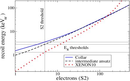
Figure 5: Different possibilities for the relation between nuclear recoil energy and number of S2 electrons observed by XENON10. Top curve (solid) is from ref. Collar:2010ht ; Collar:2011wq , bottom curve (dotted) is that used by Angle:2011th . The intermediate (dashed) curve is our hypothetical ansatz that allows for compatibility with the CoGeNT events.

III.4 XENON10

Unlike XENON100, the XENON10 experiment relinquishes its demand for scintillation photoelectrons (S1) to veto electron recoils, in order to gain a lower energy threshold and thus greater sensitivity to light dark matter. Thus one does not require a significant acceptance function, and need only consider the raw rate of nuclear recoils in energy intervals bounded by events within the range $S2=(5,43)$. This corresponds to recoil energies $E_{R}$ in the range $(E_{\rm min},\,E_{\rm max})$ where $E_{\rm min}$ is associated with the minimum number of 5 electrons imposed by the experiment as a cut on the data, and $E_{\rm max}\cong 10$ keV, whose exact value is not important for constraining light DM. XENON10 observes 23 events in this range of the S2 signal.

To set a limit, energies are assigned to each event according to the relation $S2=E_{R}{\cal Q}_{y}(E_{R})$, where ${\cal Q}_{y}(E_{R})$ is the electron yield function that must be estimated from a theoretical model. Then expected numbers of events $x_{i}$ in every energy interval bounded by two events are compared to measured events $N_{i}$ in these intervals (excluding the contributions from the endpoints), allowing for the computation of a probability $p_{i}$ that more events should have been seen than measured, based upon Poisson statistics. Finding the maximum of $p_{i}$ over all intervals and comparing to the known function $\bar{p}_{\rm Max}(C,\mu)$ leads to excluded regions in the parameter space at a specified confidence level $C$, where $\mu$ is the expected number of events in the interval $(E_{\rm min},\,E_{\rm max})$. This is the $p_{\rm Max}$ method of ref.  Yellin2002 , which was used by XENON10 to set limits on light dark matter in Angle:2011th , and in the analysis of ref. Farina:2011pw . We too use this method to compute the 90% c.l. limits from XENON10.

The crucial question is what the actual form of the electron response function ${\cal Q}_{y}$ should be, and the resulting threshold energy $E_{\rm min}$. XENON10 relies upon an extrapolation of Lindhard’s theoretical prediction below 4 keV, which leads to the estimate $E_{\rm min}=1.4$ keV. This has been criticized by refs. Collar:2010ht ; Collar:2011wq , which advocate a different prediction that leads to lower estimated sensitivity of the experiment to light DM events, and the higher threshold $E_{\rm min}=3.6$ keV. We illustrate the differences between the two estimates in fig. 5. The XENON10 version of ${\cal Q}_{y}$ leads to a strong conflict with the regions of parameter space preferred for explaining the CoGeNT signal, while the relaxed assumption removes this tension entirely. We will consider a hypothetical intermediate ansatz, also shown in fig. 5, that falls between the two estimates. In fig. 4 we show the XENON10 limits that result from the three choices of ${\cal Q}_{y}$ corresponding to fig. 5; these are the dashed (black) curves. Comparing to the CoGeNT-allowed regions, one sees that it is sufficient to choose the hypothetical intermediate ${\cal Q}_{y}$ ansatz for maintaining compatibility between CoGeNT and XENON10. We adopt this choice in what follows.

III.5 CDMS

For CDMS-Ge, we follow the procedure of ref. Farina:2011pw in assigning a $\chi^{2}$ of the form

$$\chi^{2}={(N-36)^{2}\over 36}\Theta(N-36)$$ (8)

where $N$ is the number of DM events in the relevant energy range, from the low-energy threshold of 2 keV up to 20 keV, using the efficiency for the best-performing detector T1Z5 as provided by the experiment. The ability of CDMS to distinguish 2 keV recoils from background has been disputed in ref. Collar:2011kf , which argues that 5 keV could be considered as a realistic threshold considering the uncertainties. However we are not forced to consider such a weakening of the ensuing CDMS constraints since even with 2 keV threshold, it will be seen that they do not conflict with the CoGeNT preferred regions. The previously observed tension between CoGeNT and CDMS-Ge has been alleviated by the subtraction of the CoGeNT surface contamination events, which has reduced the former “signal” events by $\sim$ 70% near the low energy threshold. In addition to including (8) in our total $\chi^{2}$ (although it makes no contribution in the relevant regions), we plot the 90% upper limit from CDMS-Ge corresponding to $45.9$ events. We have also analyzed constraints from CDMS-Si data and found them to be weaker, and therefore do not consider them henceforth.

Recently CDMS has also placed limits on a modulating DM signal in the energy range $5$-$12$ keVnr Ahmed:2012vq . However, considering the CoGeNT quenching factor, this essentially coincides with the high-energy bin in which our preferred models predict no events. Therefore we are not constrained by these data, and do not consider them in our analysis.

We note that an independent analysis of CDMS data by ref. Collar:2012ed finds an excess of low-energy events that is consistent with the CoGeNT signal. This finding is also consistent with our own observation that the CDMS constraint is the weakest of the null results, and that we did not have to make any special assumptions to achieve compatibility with the CoGeNT allowed regions that we determine below.

III.6 DAMA

We have computed the effect of DAMA’s annual modulation data on our fits, following the same procedure as in ref. Farina:2011pw . As shown in appendix B, the dipole-dipole interaction between dark matter and the target nuclei (I, Na) in the DAMA experiment can be larger than the spin-independent interaction, especially in collisions with large inelasticity. Here we compute DAMA signals including contributions from both dipole-dipole and dipole-charge interactions. The minimum value of $\chi^{2}\cong{68}$ without DAMA increases to 147 when DAMA data are included, even though only 8 data points (the number of energy bins) are included. Unlike the CoGeNT allowed region, which can be made compatible with even the most stringent conflicting data by making the judicious choices discussed above, the DAMA allowed regions are firmly ruled out. For this reason we do not try to reconcile both CoGeNT and DAMA results with the Xenon constraints. We conclude that the DAMA signal is due to some unknown background in the context of our models, as other recent studies also seem to indicate HerreroGarcia:2012fu .

Maxwellian halo	eDM	iDM	MADM
parameters	Best-fit model
$m_{\chi}$ or $m_{\mathbf{H}}$ (GeV)	9.71	8.99	9.86
$\delta_{\chi}$ or $\delta_{\mathbf{H}}$ (keV)	-	23.7	24.7
$\sigma_{\chi p}$(cm2) or $\epsilon$	$10^{-40.3}$	$10^{-37.4}$	0.029
$-D$ (cpd/kg/keVee)	0.55	0.50	0.49
$t_{0}$ (day)	205	200	198
CoGeNT	$\chi^{2}$
energy spectrum	53.9	45.4	46.4
modulation (0.5-1.5) keVee	7.60	8.58	8.94
modulation (1.5-3.1) keVee	9.36	9.40	9.47
total	70.9	63.4	64.8

Table 1: The best-fit models for CoGeNT in standard eDM, iDM, and in MADM models. All the models in the table have isospin violation $f_{n}=0$. The case of $f_{n}=f_{p}$ for eDM or iDM is the same except for decreasing $\sigma_{\chi p}$ by a factor of $(A/Z)^{2}=5.15=10^{0.71}$.

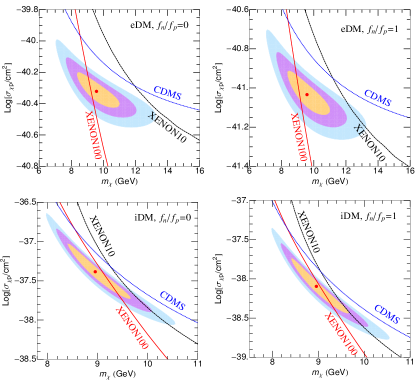
Figure 6: CoGeNT best-fit regions (shaded) in the $m_{\chi}$-$\sigma_{\chi p}$ plane, and “optimistic” 90% c.l. upper limits from XENON10, XENON100 and CDMS-Ge for eDM (top row) and iDM (bottom row) models, with isospin violation $f_{n}=0$ (leftmost graphs) or isospin conservation (rightmost graphs). The shaded regions correspond to 68.3%, 95.5% and 99.7% confidence intervals.

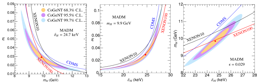
Figure 7: CoGeNT best-fit regions (shaded) for the MADM model near the benchmark point ($m_{\mathbf{H}}$, $\delta_{\mathbf{H}}$, $\epsilon$)=(9.9 GeV, 24.7 keV, 0.029). The shaded regions correspond to 68.3%, 95.5% and 99.7% confidence intervals. In each plane, the parameter that is not varying is fixed to its best-fit value.

IV Results

IV.1 Standard DM velocity distribution

We determined the regions of parameter space that give the best fits to the three models under consideration: standard elastic and inelastic dark matter (denoted as eDM and iDM, respectively), and the millicharged atomic (MADM) model. For eDM, there are just two model parameters, the DM mass $m_{\chi}$ and cross section on nucleons $\sigma_{n}$, while iDM also includes the mass splitting $\delta_{\chi}$. For MADM, we use the fractional charge $\epsilon$ to parametrize the interaction strength instead of $\sigma_{n}$, and we distinguish the mass and mass splitting from those of standard DM using $m_{\mathbf{H}}$ and $\delta m_{\mathbf{H}}$ (where ${\mathbf{H}}$ stands for the dark “hydrogen” atom). For all models, we adopt the relaxed versions of the XENON100 and XENON10 constraints corresponding to the ZEPLIN-III $0.5$-$\sigma$ lower limit on ${\cal L}_{\rm eff}$ (fig.  4) and the hypothetical intermediate ${\cal Q}_{y}$ (fig. 5), respectively.

In table 1 we display the parameters corresponding to the models that minimize the $\chi^{2}$ for the CoGeNT data (as well as CDMS although the latter gives a vanishing contribution to $\chi^{2}$ at these best fit points), as well as the corresponding minimum values of $\chi^{2}$. Inelastic DM with $m_{\chi}\cong 9$ GeV and $\delta_{\chi}\sim 24$ keV gives a significantly better fit than does elastic, and the millicharged atomic dark matter model, also inelastic, gives nearly as good a fit as iDM, with a slightly larger mass $m_{\mathbf{H}}\cong 10$ GeV and mass splitting $\delta_{\mathbf{H}}\sim 25$ keV. Due to the relatively large inelasticity, the DM-nucleon cross section in the iDM case is about 3 orders of magnitude higher than that of eDM.

For the eDM and iDM models, fig. 6 displays the CoGeNT 68.3%, 95.5% and 99.7% confidence intervals, along with the constraints from XENON10, XENON100 and CDMS, in the plane of $m_{\chi}$ and the cross section for DM scattering on protons. The XENON100 limits are the most constraining, cutting through the center of the CoGeNT allowed regions, but still leaving room for compatibility within the 68.3% c.l. intervals. The best-fit points are excluded by XENON100 for eDM but allowed for iDM. Having untuned isospin violation of the form $f_{n}=0$ (DM coupling only to protons) slightly weakens the Xenon constraints relative to the CoGeNT regions.

Next we turn to the MADM model, which we study in somewhat greater detail. The best-fit parameter set for this model is marginally consistent with XENON100, and we adopt it as our benchmark model. In table 2 we present the contributions for this model to $\chi^{2}$ from the nonmodulated and modulated data and from comparison to the DAMA annual modulation, and numbers of events expected for XENON and CDMS experiments. In figure 7, the best-fit regions and 90% c.l. constraints for MADM are displayed in the three planes $m_{\mathbf{H}}$-$\epsilon$, $\delta_{\mathbf{H}}$-$\epsilon$, and $\delta_{\mathbf{H}}$-$m_{\mathbf{H}}$, where in each case the parameter that is not varied is fixed to its benchmark value. Approximately half of the CoGeNT 68% confidence intervals are left unexcluded by the XENON100 limit, which is the most stringent of the constraints.

Experiment	Data	MADM	$\chi^{2}$
CoGeNT energy spectrum	-	-	46.5
CoGeNT modulation (0.5-1.5) keVee	-	-	8.7
CoGeNT modulation (1.5-3.1) keVee	-	-	9.4
CoGeNT total	-	-	64.7
CDMS-Ge (T1Z5), (2-20) keVnr	36	26.1	0
XENON100, $L_{\text{eff}}^{\text{central}}$	-	32.1	-
XENON100, $L_{\text{eff}}^{1\sigma}$	-	18.3	-
XENON100, $L_{\text{eff}}^{2\sigma}$	-	10.0	-
XENON100, ZEPLIN $L_{\text{eff}}^{\text{central}}$	-	5.7	-
XENON100, ZEPLIN $L_{\text{eff}}^{0.5\sigma}$	-	2.8	-
XENON100, ZEPLIN $L_{\text{eff}}^{1\sigma}$	-	1.1	-
XENON10, their ${\cal Q}_{y}$	23	49.0	-
XENON10, intermediate ${\cal Q}_{y}$	23	5.8	-
XENON10, Collar ${\cal Q}_{y}$	23	1.2	-
DAMA modulation	-	-	79

Table 2: Contributions to the total $\chi^{2}$ or to the number of events observed by CDMS-Ge or XENON experiments, for the benchmark MADM model with ($m_{\mathbf{H}}$, $\delta_{\mathbf{H}}$, $\epsilon$)=(9.9 GeV, 24.7 keV, 0.029). For the CoGeNT modulation spectrum, we include the modulating background (7). For the XENON100 and XENON10 limits, we consider various choices for ${\cal L}_{\rm eff}$ and ${\cal Q}_{y}$, discussed in section III.

IV.2 Nonstandard DM halos

We have investigated the effects of two possible modifications to the standard Maxwellian phase space density of the dark matter. The first is a distortion of the shape, of the type $f(v^{2};v_{\rm esc}^{2})\to f^{k}(v^{2}/k;v_{\rm esc}^{2}/k)$ (see eq. (13)) that has been suggested in ref. Lisanti:2010qx based upon Eddington’s relation between $f(v)$ and and the density profile $\rho(r)$. Comparisons to $N$-body simulations and to the Milky Way halo give $k=[1.5,3.5]$ and $k\sim 2$ respectively. The effects of varying $k$ on fitting to CoGeNT were previously studied in ref. Fox:2011px . We find that increasing $k$ has a relatively small effect on the best-fit regions and on the constraint curves, shifting them to somewhat higher values of DM mass and cross section, and smaller values of the mass splitting. We illustrate this for the MADM model in figure 8, where the best-fit values of the parameters and the minimum value of $\chi^{2}$ are plotted as functions of $k$.

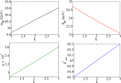
Figure 8: Dependence of best fit values of $m_{\mathbf{H}}$, $\delta_{\mathbf{H}}$, $\epsilon$ and minimum value of $\chi^{2}$ on the halo velocity profile index $k$, in the MADM model.

We next consider the debris flow scenario of ref. Kuhlen:2012fz . Tidal debris is a form of unvirialized dark matter due to tidal stripping of ubiquitous subhalos in the galaxy. Unlike tidal streams, which are rare features whose effects have been previously considered for interpreting CoGeNT in ref. Natarajan:2011gz , debris flow is argued in Kuhlen:2012fz to be homogeneously distributed in the galaxy and therefore guaranteed to be present in the solar system, with a distribution that was inferred in Kuhlen:2012fz by analysis of $N$-body simulation results.

We correct an error kuhlen in Kuhlen:2012fz by writing the full distribution function as

$$f(v)=(1-\epsilon_{0})\,f_{v}(v)+\epsilon_{0}\,f_{d}(v)$$ (9)

where $f_{v}$ is the Maxwellian distribution of the virialized component, $f_{d}$ is the contribution from debris, and $\epsilon_{0}=0.22$ is determined by comparison to $N$-body simulations. In Kuhlen:2012fz , the coefficients of $f_{v,d}$ were mistaken for functions of velocity in the computation of the DM detection rate. Ref. Kuhlen:2012fz further models $f_{d}(v)$ (in the earth frame) by an isotropic function with support in the window $v_{f}-v_{e}<v<v_{f}+v_{e}$,

$$f_{d}(v)\cong{v\over 2v_{f}\,v_{e}}\Theta(v_{f}+v_{e}-v)\Theta(v-v_{f}+v_{e})$$ (10)

where $v_{e}(t)$ is the modulating earth velocity and $v_{f}$ is a flow velocity characterizing the debris. ($f_{v,d}$ are both normalized such that $\int dvf_{v,d}=1$.) In Kuhlen:2012fz , the value $v_{f}=340$ km/s was suggested, but we find that a higher value $v_{f}=475$ km/s is required for consistency with their determination of the ratio $\epsilon(v_{\rm min})$ of debris particles to the total number of DM particles having $v>v_{\rm min}$. In fig. 9 we show that $\epsilon(v_{\rm min})$ as directly computed from eqs. (9,10) is in reasonable agreement with the result from Kuhlen:2012fz based on analysis of $N$-body simulation data, for our choice of $v_{f}$, which is definitely not the case for $v_{f}=340$ km/s. This provides a consistency check on the approximation (10) with $v_{f}=475$ km/s. The constant $\epsilon_{0}$ in (9) is equal to $\epsilon(0)$.

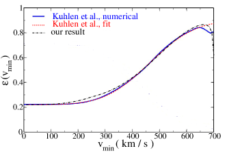
Figure 9: The ratio of debris particles to total number of dark matter particles having $v>v_{\rm min}$ in the earth frame, as determined in ref. Kuhlen:2012fz (solid and dot-dashed curves), and as calculated here, using the approximation (10) in eq. (9).

Debris flow	eDM	iDM	MADM
parameters	Best-fit model
$m_{\chi}$ or $m_{\mathbf{H}}$ (GeV)	7.4	9.8 (9.0)	10.9 (9.8)
$\delta_{\chi}$ or $\delta_{\mathbf{H}}$ (keV)	-	20.7 (23.6)	22.6 (24.8)
$\sigma_{\chi p}$(cm2) or $100\,\epsilon$	$10^{-40.9}$	$10^{-39.8}$ ($10^{-38.0}$)	0.63 (3.6)
$-D$ (cpd/kg/keVee)	0.55	$0.51$ ($0.50$)	$0.49$ ($0.49$)
$t_{0}$ (day)	205	202 (200)	199 (199)
$\chi^{2}$	71.1	59.8 (63.3)	63.9 (64.7)

Table 3: The best-fit models for CoGeNT in standard eDM and iDM and MADM models, including the debris flow component in the DM phase space distribution function. The eDM and iDM models are isospin conserving, $f_{n}=f_{p}$. Numbers in parentheses refer to the second-best fits in case of a second local minimum of $\chi^{2}$.

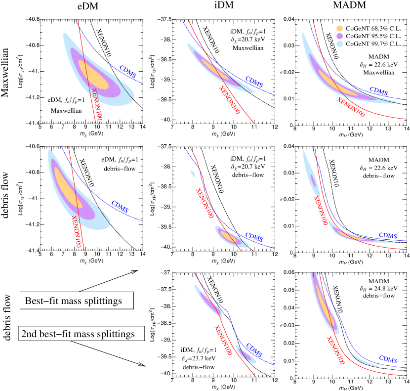
Figure 10: CoGeNT best fit regions and constraints for the eDM, iDM and MADM models (left to right) for Maxwellian DM velocity distribution (top row) and including debris flow contribution (second and third rows). The middle row sets the mass splittings to the values corresponding to the global minima of the $\chi^{2}$ for iDM and MADM, while the bottom row corresponds to the higher local minima. The eDM and iDM results are for the isospin-conserving $f_{n}=f_{p}$ case.

The debris flow contribution has interesting effects on the quality of fits and the best-fit regions for dark matter direct detection. We summarize the best-fit values in table 3. The graphical results are presented in fig. 10. In the case of isospin-conserving elastic DM, the goodness of fit is nearly unchanged, but the best-fit mass is shifted to the lower value $m_{H}=7.4$ GeV, while the cross section increases by a factor of $\sim 5$, thus moving below the region excluded by XENON100, whose constraints are also shifted, but by a lesser amount.

For inelastic DM, debris flow leads to an improvement in the best fit with $\chi^{2}=59.8$ (smaller by 3.6 than the Maxwellian halo result). The most dramatic change amongst the best-fit model parameters relative to the Maxwellian halo values is in the lower value of the cross section. There is no noticeable relative shift between the CoGeNT best-fit region and the Xenon constraints in this case. However a new local minimum with $\chi^{2}=63.3$ develops at lower $m_{\chi}$, higher $\delta_{\chi}$ and larger $\sigma_{\chi p}$. It originates from the presence of two components in $f$, only one of which dominates the signal near a given local minimum. The new low-mass region requires higher recoil velocity for a given recoil energy (especially at large mass splittings), and the debris flow contribution dominates at high $v$. A hint of this second minimum is visible in the lower middle graph of fig. 10, which has $\delta_{\chi}=20.7$ keV, the value corresponding to the global minimum, rather than the $\delta_{\chi}$ of the secondary minimum. It is clearly visible in the bottom middle graph where $\delta_{\chi}\cong 24$ keV. An interesting feature of the second minimum is that, even though its $\chi^{2}$ is higher by 3.5 than at the global minimum, it evades the Xenon constraints somewhat more robustly.

The MADM model with debris flow shares qualitative features similar to those of iDM. The best-fit $\chi^{2}$ is better (though only by 0.8) than in the Maxwellian case, the DM mass is higher, and the fractional charge $\epsilon$ is smaller. There is still a second local minimum, but in this case its mass splitting and $\chi^{2}$ are closer to that of the global minimum, so that both regions appear more clearly on the same contour plot at the global $\delta_{\mathbf{H}}$ best-fit value. Again, the secondary minimum at lower mass and higher cross section is less constrained by XENON.

IV.3 Update on XENON100 Analysis

After the first version of this paper, the XENON100 collaboration announced their new limits on DM-nucleus scattering Aprile:2012nq . In this subsection, we give an indication of how this changes our previous analysis by reconsidering only the MADM model. Here we also consider the $1\sigma$ lower limit of the ZEPLIN-III ${\cal L}_{\rm eff}$ rather than just $0.5\sigma$ as used above. Employing the maximum gap method (see Appendix D for details), we derive the limits from the new XENON100 data shown as dashed lines in fig. 11, corresponding to the $0.5\sigma$ and $1\sigma$ limits on ${\cal L}_{\rm eff}$, respectively. This figure should be compared to the leftmost graph in Fig.(7). Somewhat surprisingly, the new XENON100 $90\%$ c.l. exclusion curve crosses the previous XENON100 curve in the region of MADM parameter space shown here. The reason that they do not remain parallel at low DM mass is that events below 3 keVnr are not used in the new XENON100 analysis for exclusion limits Aprile:2012nq . Comparing the two figures, we see that the newly excluded region on MADM based on the recent XENON100 data Aprile:2012nq is nearly the same as the old one under the same ${\cal L}_{\rm eff}$ assumption.

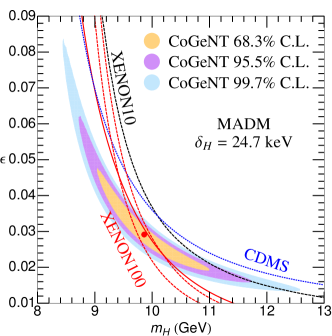
Figure 11: CoGeNT best-fit regions (shaded) for the MADM model $\delta_{\mathbf{H}}$= 24.7 keV. The two red dashed lines are the new XENON100 limits Aprile:2012nq assuming ZEPLIN-III $0.5\sigma$ and $1\sigma$ lower limits on ${\cal L}_{\rm eff}$.

V Conclusions

In this work we have attempted to find the most credible set of assumptions that would allow for a dark matter interpretation of the CoGeNT excess, without any fine-tuning of isospin-violating couplings, while remaining at least marginally consistent with constraints from null experimental results, mainly those of XENON100 and XENON10. Our focus was on standard elastic and inelastic DM (possibly having mild isospin violation $f_{n}=0$), and on a particular example of magnetic inelastic DM, the millicharged atomic DM model. Some elements of our analysis that are new relative to previous studies are: subtraction of recently identified surface-contaminated CoGeNT events; hypothesis of a modulating background, especially at high recoil energies; and consideration of an unvirialized DM debris flow component (correcting an error in the literature).

The main arguments for believing that the DM interpretation of CoGeNT can still be viable are the experimental or theoretical uncertainties in the Xenon detector response sensitivities (parametrized by the functions ${\cal L}_{\rm eff}$ and ${\cal Q}_{y}$ respectively, for XENON100 and XENON10) at low recoil energies. For XENON10 to exclude the CoGeNT preferred region, a theoretical model for ${\cal Q}_{y}$ is required Angle:2011th , which is argued to be no more plausible than an alternate model Collar:2010ht ; Collar:2011wq that leaves room for the CoGeNT allowed region. We showed that an ansatz for ${\cal Q}_{y}$ intermediate between these two extremes is also adequate for sufficiently softening the XENON10 constraint. Similarly XENON100’s ability to exclude the CoGeNT region relies upon a particular measurement and extrapolation to low energies of the relative scintillation efficiency ${\cal L}_{\rm eff}$. We showed that the assumption of an alternate ${\cal L}_{\rm eff}$, well within the error bars of another recent measurement Horn:2011wz , is sufficient to make the CoGeNT best-fit model marginally compatible with the XENON100 constraint.

While standard elastically scattering DM can still give a reasonable fit to all the data, inelastic models do better. Our featured MADM model has a different dependence upon the recoil momentum and DM velocity than standard iDM, but fits the data nearly as well as standard iDM. Our assumption of a hypothetical modulating background to explain CoGeNT modulations above $1.5$ keVee improves the $\chi^{2}$s somewhat, but our results depend quite weakly upon this feature, due to the lower statistical significance of the modulations compared to the unmodulated signal. Distortions from the Maxwellian DM distribution functions of the form (13) have a small effect on our results. However an additional contribution from debris flows (including a correction original to this paper) noticeably lowers the DM mass and relaxes the tension between eDM and XENON100, improves the fit of iDM, and has the interesting effect of introducing a second local minimum in the $\chi^{2}$ of iDM and MADM at lower DM mass, whose tension with Xenon is reduced relative to the global best-fit model.

Although our results for standard eDM and iDM models may be of primary interest for most readers, our original motivation was to study the validity, as an explanation for CoGeNT, of MADM, which appeared to be a new class of model; only in the course of this work was its similarity to other inelastic magnetic DM models noticed. But the existence of constituents with fractional electric charge $\epsilon\sim 0.01$ is a distinguishing feature of MADM, and a potentially worrisome one since early studies of similar models claimed that $\epsilon\gtrsim 10^{-3}$ is ruled out Goldberg:1986nk by searches for anomalously heavy isotopes of hydrogen. In ref. Cline:2012is we pointed out several possible loopholes to this constraint, including the fact that the screening effect of the earth’s magnetosphere on the subdominant ionized component of the dark matter has not been taken into account in its derivation. Subsequent to the publication of Cline:2012is , we have received confirmation from some of the authors on the heavy isotope search papers klein_etal ; hemmick_etal that the sensitivity of these searches to isotopes with charges deviating from exact integer values could have been significantly reduced hkp . We therefore keep an open mind about the viability of MADM even with fractional charges as large as $\sim 0.01$ as we find necessary for explaining CoGeNT. It could be interesting to reinvestigate in more detail what values of $\epsilon$ are consistent with existing searches for charged relics.

Based on these results, we remain optimistic that CoGeNT may really be detecting dark matter of mass $\sim 10$ GeV, and perhaps with inelastic couplings between states split by $\sim 20$ keV. New data expected from CoGeNT in the near future should shed further light on this exciting possibility.

Appendix A dark matter velocity distributions

The velocity distribution function for the standard Maxwellian halo is often taken to be

$$f=N\left(e^{-v^{2}/v_{0}^{2}}-e^{-v_{\rm esc}^{2}/v_{0}^{2}}\right)$$ (11)

with

$$N^{-1}=4\pi v_{0}^{3}\left({\sqrt{\pi}\over 4}{\rm erf}(a)-ae^{-a^{2}}\left(\frac{1}{2}+\frac{1}{3}a^{2}\right)\right)$$ (12)

where $a=v_{\rm esc}/v_{0}$. Standard values are $v_{0}=220$ km/s, $v_{\rm esc}=500-600$ km/s, $v_{e}=232\pm 30$ where $\pm 15.3$ is the range of annual variation. (The earth’s velocity relative to the DM barycenter appears in $f(\vec{v}+\vec{v}_{e})$ when computing nuclear recoil rates.) Unless otherwise noted, we adopt $v_{\rm esc}=600$ in computing detection rates.

In addition to this standard form, we also consider a generalized expression with the extra parameter $k$,

$$f_{k}=N_{k}\left(e^{-v^{2}/kv_{0}^{2}}-e^{-v_{\rm esc}^{2}/kv_{0}^{2}}\right)^{k}$$ (13)

with normalization factor

$$N_{k}^{-1}=4\pi\int_{0}^{v_{\rm esc}}dv\,v^{2}\,\left(e^{-v^{2}/kv_{0}^{2}}-e^{-v_{\rm esc}^{2}/kv_{0}^{2}}\right)^{k}$$ (14)

which has no closed-form expression except for integral values of $k$.

Appendix B Direct detection rate

In this appendix we give details of the derivation of differential scattering on nuclei for MADM through spin-independent (dipole-charge) and spin-dependent (dipole-dipole) interactions. The differential detection rate for either case is given by

$${dR\over dE_{R}}={2\pi N_{T}m_{N}\rho_{\mathbf{H}}\over m_{\mathbf{H}}\,\mu^{2}}\int_{v_{\rm min}}{d^{\,3}v\over v^{\prime}}f(v){d\sigma_{N}\over d\Omega}$$ (15)

where $v^{\prime}=\sqrt{v^{2}-y}$ is the final velocity, with $y\equiv 2\delta_{\mathbf{H}}/\mu$. The average matrix element squared for dipole-charge scattering is given by Cline:2012is

$$(C/q)^{2}|\vec{v}\times\hat{q}|^{2}(\mu/p)$$ (16)

where $C=Z\epsilon e^{2}/m_{{\mathbf{e}}}$. The differential cross section for the dipole-charge interaction is given by

$${d\sigma_{N}\over d\Omega} = \left({4\epsilon\alpha Z\over m_{\mathbf{H}}}\right)^{2}{\mu^{4}vv^{\prime 3}\over q^{4}}\sin^{2}\theta\,F_{H}^{2}$$ (17)

$$= \left({4\epsilon\alpha Z\over m_{\mathbf{H}}}\right)^{2}\sqrt{1-{y\over v^{2}}}\,\left(v^{2}-v_{\rm min}^{2}\right)\,{F_{H}^{2}\over x}$$

where we defined $x\equiv q^{2}/\mu^{2}$ and used the relations

$$\sin^{2}\theta={x(v^{2}-v_{\rm min}^{2})\over v^{2}(v^{2}-y)},\quad v_{\rm min}={x+y\over 2\sqrt{x}}$$ (18)

Then the rate due to dipole-charge interaction can be written as

$$\frac{dR_{\text{DZ}}}{dE_{R}}=\frac{N_{T}\rho_{\mathbf{H}}\pi}{m_{\mathbf{H}}}\left(4\epsilon\alpha\over m_{\mathbf{H}}\right)^{2}\frac{Z^{2}F_{H}^{2}}{E_{R}}\left\langle\frac{v^{2}-v_{\text{min}}^{2}}{v}\right\rangle$$ (19)

where the velocity integral is given by

$$\left\langle\frac{v^{2}-v_{\text{min}}^{2}}{v}\right\rangle=\int_{v_{\rm min}}{d^{\,3}v}\left(v^{2}-v_{\rm min}^{2}\over v\right)f(\vec{v}+\vec{v}_{e})$$ (20)

with $\vec{v}_{e}$ the earth’s velocity relative to the halo.

For the dipole-dipole interaction, we consider the Hamiltonian

$$H_{\rm int}={\epsilon e\over 3m_{{\mathbf{e}}}}(\vec{\sigma}_{{\mathbf{e}}}-\vec{\sigma}_{{\mathbf{p}}})\cdot\vec{\mu}_{N}\,\delta^{(3)}(\vec{r}_{\mathbf{H}}-\vec{r}_{N})$$ (21)

where the $\sigma$’s are Pauli matrices corresponding to the spins of ${\mathbf{p}}$ and ${\mathbf{e}}$, and $\vec{\mu}_{N}$ is the magnetic moment of the nucleus. The spin-summed squared matrix element is

$$\sum|\langle f|H_{\rm int}|i\rangle|^{2}=\frac{4}{9}\left({I+1\over I}\right)\left(\epsilon e\mu_{N}\over m_{{\mathbf{e}}}\right)^{2}(\mu/p)$$ (22)

The differential detection rate due to dipole-dipole scattering is

$$\begin{split}\frac{dR_{\text{DD}}}{dE_{R}}&=\frac{N_{T}\rho_{\mathbf{H}}\pi}{m_{\mathbf{H}}}\left(4\epsilon\alpha\over m_{\mathbf{H}}\right)^{2}\left\langle\frac{1}{v}\right\rangle\frac{2m_{N}F_{M}^{2}}{9m_{p}^{2}}\sum_{i}f_{i}\hat{\mu}_{i}^{2}\frac{I_{i}+1}{I_{i}}\end{split}$$ (23)

where the summation is over possible isotopes of the target nucleus, $f_{i}$ is the relative abundance, $\hat{\mu}_{i}$ is the magnetic moment of isotope $i$ in units of $e/2m_{p}$, and $I_{i}$ is the spin. $F_{M}$ is the form factor for the nuclear spin. In the following estimates we will assume that $F_{M}\cong F_{H}$. The ratio of (23) to (19) is

$$R=\sum_{i}R_{i}\equiv\left(qF_{M}\over 3m_{p}ZF_{H}\right)^{2}F(v_{\text{min}})\sum_{i}f_{i}\hat{\mu}_{i}^{2}\frac{I_{i}+1}{I_{i}}$$ (24)

where the function $F$ is given by

$$F(v_{\text{min}})\equiv\left\langle\frac{1}{v}\right\rangle/\left\langle\frac{v^{2}-v_{\text{min}}^{2}}{v}\right\rangle$$ (25)

When $v_{\text{min}}<$ 500 km/s, $F(v_{\text{min}})/10^{6}\sim$(1-1.4). For large $v_{\text{min}}$ values, $F(600,700,750,800)/10^{6}$ = (1.6, 2.2, 3.1, 7.2). Taking $q=20$ MeV, $\delta_{\mathbf{H}}=25$ keV, $m_{\mathbf{H}}=10$ GeV, we find $R_{i}\sim(7.1/Z)^{2}(F/10^{6})f_{i}\hat{\mu}_{i}^{2}(I_{i}+1)/I_{i}$. We list these values in the last colummn of table 4.

Table 4: Relevant isotopes, atomic number, abundances, spins, magnetic moments (in units of $e/2m_{p}$), minimum velocity for $(q,m_{\mathbf{H}},\delta_{\mathbf{H}})$=(20 MeV, 10 GeV, 25 keV), function $F(v_{\text{min}})$, ratio of dipole-dipole to dipole-charge scattering. The values of $\mu_{N}$ can be found at magneticdipole .

isotope	$Z$	%	spin	$\hat{\mu}_{N}$	$v_{\text{min}}$	$F/10^{6}$	$R_{i}$
23Na	11	100	$3/2$	$2.218$	815	13.2	45
73Ge	32	7.7	$9/2$	$-0.879$	719	2.5	0.009
127I	53	100	$5/2$	$2.813$	700	2.2	0.4
129Xe	54	26.4	$1/2$	$-0.778$	700	2.2	0.02
131Xe	54	21.2	$3/2$	$0.692$	700	2.2	0.006

We have checked these estimates more quantitatively by computing the energy spectra due to dipole-dipole (DD) and dipole-charge (DZ) scattering in the MADM model ($m_{\mathbf{H}},\delta_{\mathbf{H}},\epsilon$)=(9.9 GeV, 24.7 keV, 0.029). In the CoGeNT and CDMS experiments, the DD interaction contributes about 1% of the total rate. In the XENON100 experiment, the signal due to DD is about 5% of the total. For collisions on iodine in DAMA, the DD spectrum has roughly the same magnitude as DZ, but most of the recoil events have energies below the region of interest. The DD spectrum is about 20 times larger than that of DZ for collisions on Na in the DAMA experiment. The recoil spectra on Na due to DD and DZ were also compared for the elastic case ($\delta_{\mathbf{H}}=0$), in which case the two contributions are of comparable size. We conclude that the DD interaction is important for the DAMA analysis, especially for scenarios with large inelasticity.

Appendix C XENON100 acceptance

In XENON100, the relative scintillation efficiency ${\cal L}_{\rm eff}$ is important for determining the mean number of S1 photoelectrons corresponding to a given nuclear recoil energy, through the relation

$$\mu_{S1}(E_{R})=\left(\frac{S_{nr}}{S_{ee}}\right)\,\mathcal{L}_{\text{eff}}(E_{R})\,L_{y}\,E_{R}\ .$$ (26)

where $S_{ee}=0.58$ and $S_{nr}=0.95$ Aprile:2006kx are the suppression in the scintillation yield for electronic and nuclear recoil respectively, and the light yield $L_{y}=2.20$ PE/keV_ee is normalized at 122 keV_ee Aprile:2010um . The uncertainties in these parameters are negligible compared to that of ${\cal L}_{\rm eff}$.

In order to use the experiment to constrain DM models, one could follow the likelihood method introduced in Aprile:2011hx . A simpler method (similar to the one we adopt) is described in the thesis Felixthesis , which requires the acceptance function $A(E_{R})$, that enters in the number of expected DM events in a given energy range $(E_{1},E_{2})$ as

$$N={\cal E}\int_{E_{1}}^{E_{2}}\frac{\mathrm{d}R}{\mathrm{d}E_{R}}A(E_{R})\,\mathrm{d}E_{R}$$ (27)

where ${\cal E}=4843.2$ kg$\cdot$d is the exposure. The acceptance function takes account of $\mathcal{L}_{\text{eff}}$, the Poisson fluctuations of the $S1$ signal, and the acceptance of the $S1$ and the nuclear recoil cut $\zeta_{\rm cut}(n_{1})$ Aprile:2011hi ,

$$A(E_{R})=\sum_{n_{1}=S1_{\rm min}}^{S1_{\rm max}}P\left(n_{1},\mu_{S1}(E_{R})\right)\zeta_{\rm cut}(n_{1})$$ (28)

where $\mu_{S1}(E_{R})$ is given in eq. (26) and the S1 window used by XENON100 is $S1_{\rm min}=4$, $S1_{\rm max}=30$. The acceptance of the applied cuts $\zeta_{\rm cut}$ is the product of the data quality cut and S2/S1 electron recoil discrimination cut, shown in fig. 2 of ref. Aprile:2011hi . The data quality cut depends upon the DM mass, and we interpolate between the curves given in Aprile:2011hi . $P$ is the Poisson distribution,

$$P\left(n_{1},\mu_{S1}(E_{R})\right)={\mu_{S1}(E_{R})^{n_{1}}e^{-\mu_{S1}(E_{R})}}/{n_{1}!}\ .\phantom{{{{|_{|}}_{|}}_{|}}_{|}}$$ (29)

To compute an upper limit from the number of events, we use the maximum gap method of ref. Yellin2002 , which as described in sect. III.3 restricts $N<3.1$ at 90% c.l. in the energy window 8.4–12.1 keVnr.

Appendix D XENON100 analysis (2012 Data)

Two DM candidate events with $3.3$ PE and $3.8$ PE were observed in XENON100 data Aprile:2012nq , which partition the search region S1=(3-20) PE into 3 gaps for the maximum gap analysis: (3-3.3), (3.3-3.8), and (3.8-20). The predicted DM events in each gap are computed via the acceptance function $A_{i}(E_{R})$

$$N_{i}=\mathcal{E}\int\frac{dR}{dE_{R}}(E_{R})A_{i}(E_{R})dE_{R}$$ (30)

where $i=1,2,3$ and $\mathcal{E}=$ 34 kg $\times$ 224.6 days. The acceptance function $A_{i}(E_{R})$ is given by

$$\begin{split}A_{i}(E_{R})=&\epsilon_{S2}(E_{R})\sum_{N_{pe}=1}^{\infty}P(N_{pe},\mu_{S1}(E_{R}))\\ \times&\int_{S1^{i}_{\text{min}}}^{S1^{i}_{\text{max}}}\epsilon_{S1}(S1)G(S1,N_{pe})dS1\end{split}$$ (31)

where $\epsilon_{S2}(E_{R})$ and $\epsilon_{S1}(S1)$ are the efficiency functions for $S2$ and $S1$ signals respectively which are digitized from Aprile:2012nq . $P(N_{pe},\mu_{S1}(E_{R}))$ is given in Eq.(29). $G(S1,N_{pe})$ is a Gaussian distribution describing the response of the PMTs

$$\text{G}(S1,N_{pe})=\frac{1}{\sqrt{2\pi}}\frac{1}{\sigma_{\text{PMT}}\sqrt{N_{pe}}}\exp\left[-\frac{1}{2}\left(\frac{S1-N_{pe}}{\sigma_{\text{PMT}}\sqrt{N_{pe}}}\right)^{2}\right]$$ (32)

where $\sigma_{\text{PMT}}$=0.5 PE Aprile:2012vw .

To compute the exclusion limits in maximum gap method Yellin2002 , we use the number of DM events calculated here together with the expected background events, (1.0$\pm$0.2) Aprile:2012nq .

References

- (1) R. Bernabei et al. [DAMA Collaboration], Eur. Phys. J. C 56 (2008) 333 [arXiv:0804.2741 [astro-ph]].
- (2) C. E. Aalseth et al. [CoGeNT Collaboration], Phys. Rev. Lett. 106, 131301 (2011) [arXiv:1002.4703].
- (3) C. E. Aalseth, P. S. Barbeau, J. Colaresi, J. I. Collar, J. Diaz Leon, J. E. Fast, N. Fields and T. W. Hossbach et al., Phys. Rev. Lett. 107, 141301 (2011) [arXiv:1106.0650 [astro-ph.CO]].
- (4) G. Angloher, M. Bauer, I. Bavykina, A. Bento, C. Bucci, C. Ciemniak, G. Deuter, F. von Feilitzsch et al., [arXiv:1109.0702 [astro-ph.CO]].
- (5) A. L. Fitzpatrick, D. Hooper and K. M. Zurek, Phys. Rev. D 81, 115005 (2010) [arXiv:1003.0014 [hep-ph]].
- (6) S. Andreas, C. Arina, T. Hambye, F. -S. Ling and M. H. G. Tytgat, Phys. Rev. D 82, 043522 (2010) [arXiv:1003.2595 [hep-ph]].
- (7) R. Foot, Phys. Lett. B 692, 65 (2010) [arXiv:1004.1424 [hep-ph]].
- (8) V. Barger, M. McCaskey and G. Shaughnessy, Phys. Rev. D 82, 035019 (2010) [arXiv:1005.3328 [hep-ph]].
- (9) K. J. Bae, H. D. Kim and S. Shin, Phys. Rev. D 82, 115014 (2010) [arXiv:1005.5131 [hep-ph]].
- (10) Y. Mambrini, JCAP 1009, 022 (2010) [arXiv:1006.3318 [hep-ph]].
- (11) D. Hooper, J. I. Collar, J. Hall, D. McKinsey and C. Kelso, Phys. Rev. D 82, 123509 (2010) [arXiv:1007.1005 [hep-ph]].
- (12) A. L. Fitzpatrick and K. M. Zurek, Phys. Rev. D 82, 075004 (2010) [arXiv:1007.5325 [hep-ph]].
- (13) J. M. Cline, A. R. Frey and F. Chen, Phys. Rev. D 83, 083511 (2011) [arXiv:1008.1784 [hep-ph]].
- (14) A. V. Belikov, J. F. Gunion, D. Hooper and T. M. P. Tait, Phys. Lett. B 705, 82 (2011) [arXiv:1009.0549 [hep-ph]].
- (15) J. F. Gunion, A. V. Belikov and D. Hooper, arXiv:1009.2555 [hep-ph].
- (16) M. R. Buckley, D. Hooper and T. M. P. Tait, Phys. Lett. B 702, 216 (2011) [arXiv:1011.1499 [hep-ph]].
- (17) E. Del Nobile, C. Kouvaris and F. Sannino, Phys. Rev. D 84, 027301 (2011) [arXiv:1105.5431 [hep-ph]].
- (18) D. Hooper and C. Kelso, Phys. Rev. D 84, 083001 (2011) [arXiv:1106.1066 [hep-ph]].
- (19) J. M. Cline and A. R. Frey, Phys. Rev. D 84, 075003 (2011) [arXiv:1108.1391 [hep-ph]].
- (20) C. Kelso, D. Hooper and M. R. Buckley, Phys. Rev. D 85, 043515 (2012) [arXiv:1110.5338 [astro-ph.CO]].
- (21) R. Foot, arXiv:1203.2387 [hep-ph].
- (22) J. Angle et al. [XENON10 Collaboration], Phys. Rev. Lett. 107, 051301 (2011) [arXiv:1104.3088].
- (23) E. Aprile et al. [XENON100 Collaboration], Phys. Rev. Lett. 107, 131302 (2011) [arXiv:1104.2549].
- (24) Z. Ahmed et al. [The CDMS-II Collaboration], Science 327, 1619 (2010) [arXiv:0912.3592 [astro-ph.CO]].
- (25) Z. Ahmed et al. [CDMS-II Collaboration], Phys. Rev. Lett. 106, 131302 (2011) [arXiv:1011.2482 [astro-ph.CO]].
- (26) Z. Ahmed et al. [CDMS Collaboration], arXiv:1203.1309 [astro-ph.CO].
- (27) E. Armengaud et al. [EDELWEISS Collaboration], arXiv:1207.1815 [astro-ph.CO].
- (28) M. T. Frandsen, F. Kahlhoefer, J. March-Russell, C. McCabe, M. McCullough, K. Schmidt-Hoberg, [arXiv:1105.3734 [hep-ph]].
- (29) T. Schwetz, J. Zupan, [arXiv:1106.6241 [hep-ph]].
- (30) M. Farina, D. Pappadopulo, A. Strumia, T. Volansky, [arXiv:1107.0715 [hep-ph]].
- (31) P. J. Fox, J. Kopp, M. Lisanti, N. Weiner, [arXiv:1107.0717 [hep-ph]].
- (32) C. McCabe, Phys. Rev. D 84, 043525 (2011) [arXiv:1107.0741 [hep-ph]].
- (33) C. Arina, J. Hamann, R. Trotta and Y. Y. Y. Wong, JCAP 1203, 008 (2012) [arXiv:1111.3238 [hep-ph]].
-
(34)
J. Collar, presentation at UCLA Dark Matter 2012,
https://hepconf.physics.ucla.edu/dm12/ - (35) J. M. Cline, Z. Liu and W. Xue, arXiv:1201.4858 [hep-ph].
- (36) D. E. Kaplan, G. Z. Krnjaic, K. R. Rehermann and C. M. Wells, JCAP 1005, 021 (2010) [arXiv:0909.0753 [hep-ph]].
- (37) D. E. Kaplan, G. Z. Krnjaic, K. R. Rehermann and C. M. Wells, JCAP 1110, 011 (2011) [arXiv:1105.2073 [hep-ph]].
- (38) S. Chang, N. Weiner and I. Yavin, Phys. Rev. D 82, 125011 (2010) [arXiv:1007.4200 [hep-ph]].
- (39) M. Pospelov and T. ter Veldhuis, Phys. Lett. B 480, 181 (2000) [hep-ph/0003010].
- (40) K. Sigurdson, M. Doran, A. Kurylov, R. R. Caldwell and M. Kamionkowski, Phys. Rev. D 70, 083501 (2004) [Erratum-ibid. D 73, 089903 (2006)] [astro-ph/0406355].
- (41) J. H. Heo, Phys. Lett. B 693, 255 (2010) [arXiv:0901.3815 [hep-ph]].
- (42) E. Masso, S. Mohanty and S. Rao, Phys. Rev. D 80, 036009 (2009) [arXiv:0906.1979 [hep-ph]].
- (43) W. S. Cho, J. -H. Huh, I. -W. Kim, J. E. Kim and B. Kyae, Phys. Lett. B 687, 6 (2010) [Erratum-ibid. B 694, 496 (2011)] [arXiv:1001.0579 [hep-ph]].
- (44) V. Barger, W. -Y. Keung and D. Marfatia, Phys. Lett. B 696, 74 (2011) [arXiv:1007.4345 [hep-ph]].
- (45) K. Kumar, A. Menon and T. M. P. Tait, JHEP 1202, 131 (2012) [arXiv:1111.2336 [hep-ph]].
- (46) T. Lin and D. P. Finkbeiner, Phys. Rev. D 83, 083510 (2011) [arXiv:1011.3052 [astro-ph.CO]].
- (47) S. Patra and S. Rao, arXiv:1112.3454 [hep-ph].
- (48) N. Weiner and I. Yavin, arXiv:1206.2910 [hep-ph].
- (49) E. Del Nobile, C. Kouvaris, P. Panci, F. Sannino and J. Virkajarvi, arXiv:1203.6652 [hep-ph].
- (50) M. Lisanti, L. E. Strigari, J. G. Wacker and R. H. Wechsler, Phys. Rev. D 83, 023519 (2011) [arXiv:1010.4300 [astro-ph.CO]].
- (51) M. Lisanti and D. N. Spergel, arXiv:1105.4166 [astro-ph.CO].
- (52) M. Kuhlen, M. Lisanti and D. N. Spergel, arXiv:1202.0007 [astro-ph.GA].
- (53) P. Salucci, F. Nesti, G. Gentile and C. F. Martins, Astron. Astrophys. 523, A83 (2010) [arXiv:1003.3101 [astro-ph.GA]].
- (54) J. D. Lewin and P. F. Smith, Astropart. Phys. 6, 87 (1996).
- (55) S. Chang, J. Liu, A. Pierce, N. Weiner and I. Yavin, JCAP 1008, 018 (2010) [arXiv:1004.0697 [hep-ph]].
- (56) J. L. Feng, J. Kumar, D. Marfatia and D. Sanford, Phys. Lett. B 703, 124 (2011) [arXiv:1102.4331 [hep-ph]].
- (57) H. An and F. Gao, arXiv:1108.3943 [hep-ph].
- (58) J. Collar, Private communication
- (59) J. N. Bahcall, Phys. Rev. 132, 362 (1963).
- (60) M. Horn, V. A. Belov, D. Y. .Akimov, H. M. Araujo, E. J. Barnes, A. A. Burenkov, V. Chepel and A. Currie et al., Phys. Lett. B 705, 471 (2011) [arXiv:1106.0694 [physics.ins-det]].
- (61) F. Kahlhoefer, “Sensitivity of Liquid Xenon Detectors for Low Mass Dark Matter,” diploma thesis, unpublished (2010).
- (62) E. Aprile et al. [XENON100 Collaboration], Phys. Rev. D 84, 052003 (2011) [arXiv:1103.0303 [hep-ex]].
- (63) S. Yellin, Phys. Rev. D 66, 032005 (2002)
- (64) C. Savage, G. Gelmini, P. Gondolo and K. Freese, Phys. Rev. D 83, 055002 (2011) [arXiv:1006.0972 [astro-ph.CO]].
- (65) J. I. Collar, arXiv:1006.2031 [astro-ph.CO].
- (66) G. Plante, E. Aprile, R. Budnik, B. Choi, K. L. Giboni, L. W. Goetzke, R. F. Lang and K. E. Lim et al., Phys. Rev. C 84, 045805 (2011) [arXiv:1104.2587 [nucl-ex]].
- (67) J. I. Collar, arXiv:1106.0653 [astro-ph.CO].
- (68) V. N. Lebedenko, H. M. Araujo, E. J. Barnes, A. Bewick, R. Cashmore, V. Chepel, A. Currie and D. Davidge et al., Phys. Rev. D 80, 052010 (2009) [arXiv:0812.1150 [astro-ph]].
- (69) J. I. Collar, arXiv:1010.5187 [astro-ph.IM].
- (70) J. I. Collar, arXiv:1103.3481 [astro-ph.CO].
- (71) J. I. Collar and N. E. Fields, arXiv:1204.3559 [astro-ph.CO].
- (72) J. Herrero-Garcia, T. Schwetz and J. Zupan, arXiv:1205.0134 [hep-ph].
- (73) A. Natarajan, C. Savage and K. Freese, Phys. Rev. D 84, 103005 (2011) [arXiv:1109.0014 [astro-ph.CO]].
- (74) M. Lisanti and M. Kuhlen, private communication
- (75) H. Goldberg and L. J. Hall, Phys. Lett. B 174, 151 (1986).
- (76) J. Klein, R. Middleton and W.E. Stephens, in ANL Symposium on Accelerator Mass Spectroscopy (1981).
- (77) T. K. Hemmick, D. Elmore, T. Gentile, P.W. Kubik, S.L. Olsen, D. Ciampa, D. Nitz and H. Kagan et al., Phys. Rev. D 41, 2074 (1990).
- (78) T.K. Hemmick, private communication; J. Klein, private communication.
- (79) E. Aprile, C. E. Dahl, L. DeViveiros, R. Gaitskell, K. L. Giboni, J. Kwong, P. Majewski and K. Ni et al., Phys. Rev. Lett. 97, 081302 (2006) [astro-ph/0601552].
- (80) E. Aprile et al. [XENON100 Collaboration], Phys. Rev. Lett. 105, 131302 (2010) [arXiv:1005.0380 [astro-ph.CO]].
- (81) E. Aprile et al. [XENON100 Collaboration], arXiv:1207.3458 [astro-ph.IM].
- (82) E. Aprile et al. [XENON100 Collaboration], Phys. Rev. Lett. 109, 181301 (2012) [arXiv:1207.5988 [astro-ph.CO]].
- (83) http://www.webelements.com/