Stochastic particle packing with specified granulometry and porosity

Abstract

This work presents a technique for particle size generation and placement in arbitrary closed domains. Its main application is the simulation of granular media described by disks. Particle size generation is based on the statistical analysis of granulometric curves which are used as empirical cumulative distribution functions to sample from mixtures of uniform distributions. The desired porosity is attained by selecting a certain number of particles, and their placement is performed by a stochastic point process. We present an application analyzing different types of sand and clay, where we model the grain size with the gamma, lognormal, Weibull and hyperbolic distributions. The parameters from the resulting best fit are used to generate samples from the theoretical distribution, which are used for filling a finite-size area with non-overlapping disks deployed by a Simple Sequential Inhibition stochastic point process. Such filled areas are relevant as plausible inputs for assessing Discrete Element Method and similar techniques.

1 Introduction

The Discrete Element Method (DEM) has become a powerful tool in the numerical simulation of engineering problems involving discontinuous media. Among the problems where the method has been applied, we may cite fragmentation, fracture, impact, and collision phenomena, in addition to those directly related to soil modeling as part of studies of geomechanical problems cundall88 ; cundall79 ; zarate01 ; zarate04 .

DEMs are based on media discretization into finite sets of particles. More often than not, this discretization must satisfy some requirements. In order to achieve significant results, a good representation of the studied media is needed and, therefore, the particle generation must meet the granulometric curves of soil and should be as close as possible to the specified porosity. A general procedure would be then comprised of two stages, namely, (i) particle size generation, and (ii) particle placement.

The measurement of particle size is an activity that is common to diverse disciplines: archaeology, fuel technology, medicine, geology, sedimentology, civil engineering, pharmacology, etc. The common objective is to determine the overall size distribution of a collection of particles Fieller1992 . Particle-size distribution (PSD) is fundamental for characterizing construction materials, soil mechanics, soil physics, sediment-flux in rivers, and others. In soil science, it is typically presented as the percentage of the total mass of soil occupied by a given size fraction. Determination of the soil PSD is not a trivial task because of the heterogeneity of the shape and density of particles Eshel2004 . Classical techniques used to determine the PSD, like sieving and sedimentation, are point-wise and, thus, require an interpolation to obtain the complete PSD curve. The transformation of discrete points into continuous functions can be made by mathematical models daSilva2004 , where the normal, lognormal and Weibull distributions are especially prevalent Fieller1992 .

The PSD in soils is frequently assumed to be approximately lognormal Buchan1989 ; Shirazi1984 , but there are soils which present bimodal PSDs Walker1986 . A bimodal lognormal Gaussian distribution is presented in Shiozawa1991 for the characterization of various soil samples. It consists of a weighted sum of two distributions: primary minerals (sand and silt), and secondary minerals (clay), each described by a Gaussian law.

Besides the lognormal distributions, other models have been proposed, including one based on the water retention curve Fredlund2000 , the Gompertz model Nemes1999 , the fragmentation model Bittelli1999 and estimating the PSD from limited soil texture data Skaggs2001 . Furthermore, the modelling of PSD by means of the fractal mass distribution is presented in Martin1998 . Combining some well-founded theoretical results from fractal geometry, the model allows to simulate the PSD of a given soil and its characterization by means of the entropy dimension.

Although statisticians have ocasionally examined particular problems with the estimation of PSD Fisher1923 , it was not until the work of Barndorff-Nielsen1977 that a coherent statistical approach was formulated. That paper introduced the log-hyperbolic distribution as a suitable model for particle sizes. However, the considerable computational difficult involved in fitting this model has prevented it from achieving widespread use Fieller1992 .

The comparison of mathematical models for fitting PSD curves in soil science has been performed in a few works Buchan1993 ; daSilva2004 ; Hwang2002 ; Rousseva1997 . On the studies of Hwang2002 , seven parametric models were tested – the majority lognormal models and growing curves type – including a unimodal and six bimodal models. They compare five lognormal models with one, two and three parameters Buchan1993 , the Gompertz model with four parameters Nemes1999 and the Fredlund model with four parameters Fredlund2000 using 1387 Corean soil samples. Four comparison techniques were considered to define the best model: the coefficient of determination ($R^{2}$), the $F$ statistic, the $C_{p}$ statistic of Mallows Mallows1973 and the Akaike’s information criterion (AIC). They conclude that the Fredlund model presented the best fit for the majority of the soils studied, with increasing performance with the increase of clay content. Furthermore, they showed that texture could affect the performance of the PSD models. This work represents an important contribution to the model comparison for fitting granulometric data, but another models, potencially adaptable to this finality were not studied. Moreover, the authors compared models with different number of parameters; this could be a problem because it can benefit those more degrees of freedom daSilva2004 .

The work done by daSilva2004 tested and compared fourteen different models with feasibility to fit the cumulative PSD curve based on four measured points. The parameter used to compare the models was the sum of the square errors between the measured and calculated values. They concluded that the most recommendable models to fit PSD curves were: Skaggs model Skaggs2001 , Weibull model Weibull1951 and Morgan model Morgan1975 , all of them with three parameters.

In this work we transform data from granulometric curves into unevenly spaced histograms, and then sample from this empirical distribution. The sampled data is explained by means of four distributions, namely the hyperbolic, gamma, log-normal and Weibull laws, and the best fit is associated to the original granulometric curve. We then obtain an arbitrary number of radii sampling from the chosen distribution, and we place these particles in an arbitrary closed region of the plane or the space, using a stochastic point process. The number of particles to be used is iteratively determined in order to satisfy a predefined porosity.

Many procedures have been presented for particle placement with well-known tractable shapes, especially disks and balls (spheres) for the two or three- dimensional cases, respectively. These procedures are generally divided into two distinct groups: geometric and dynamic algorithms.

Dynamic algorithms use mechanical procedures that reproduce external actions to achieve an initial set of particles. A typical approach of these algorithms consists of creating a regular array of particles and them randomly disorder it through the action of gravitational forces feng03 . Other approaches require the use of DEM simulation procedures in order to achieve the initial configuration.

These dynamic approaches have many advantages, including the possibility of filling any arbitrary-geometrical domain with elements of predefined, irregular sizes and, still, controlling the desired porosity. An overview of typical dynamic techniques can be found in Cui03 ; feng03 . However, in most cases, these dynamic algorithms require checking of contacts between particles to achieve the desired result, making them significantly slower in terms of computational cost.

Another category of techniques is based on geometric algorithms. These algorithms are characterized by the use of purely geometric concepts for generating particles in a given domain, without the need of dynamic simulations to represent their movement and interactions. This often reduces significantly the processing time. The literature of granular media offers several techniques for random generation of disks or spheres with different diameters. One of the main strategies consists on establishing the position and the size of particles from random numbers. If there is overlap, a new random location is performed with the same fixed size PFC2D ; Lin1997Geotechnique .

Other geometric techniques are based on particle generation from an initial triangular or tetrahedrons elements mesh, and placing disks or spheres in the interior of these elements Cui03 . Several other geometric strategies can be found in the literature, including those that use the concept of boundary contraction, where the particle locations are calculated from the previous inclusion of other particles with a pre-established diameter Bagi2005GranularMatter ; Labra2008CommunicationsinNumericalMethodsinEngineering ; Lohner2004InternationalJournalforNumericalMethodsinEngineering .

The class of Random Sequential Adsorption – RSA processes describes the deposition of particles. Variations include the dimension and other properties of the substrate, the shape of the particles and how they interact among them and with the media DynamicsNonequilibriumDepositionPrivman . An important characteristic of our work is that we use random particle sizes. Quoting Cadilhe et al RandomSequentialAdsorption :

Versions of the continuum RSA model with deposition of mixtures of particles of different sizes and shapes have only been studied for the simplest cases of two particle sizes and identical shapes. […] In spite of all the research work thus far, the field remains widely open to new research efforts.

Dynamic algorithms grant the simulation of samples which are in geostatic balance with spatial homogeneity, and either specified granulometry or prosity, at the expense of high computational cost. Geometric algorithms are much faster than the former, but they do not grant geostatic balance. The latter are, thus, more adequate in, for instance, Monte Carlo techniques. Moreover, traditional geometric algorithms have difficulties in reaching answers that meet the specified granulometric curves.

This work presents a geometric technique for particle size generation and placement in arbitrary closed domains. Its main application is the simulation of granular media described by disks which can be extended to spheres. Particle size generation is based on the statistical analysis of granulometric curves. These curves are treated as empirical cumulative distribution functions, histograms are derived from them, and each bin is used as the density of a uniform random variable. Samples from these uniform laws are then obtained. The desired porosity is attained by selecting a certain number of particles, and their placement is performed by a stochastic point process. This proposal grants both porosity and granulometric properties with spatial homogeneity, i.e, the system is in global equilibrium as in fully saturated porous media (see Figure 1). On the one hand, by construction, the results adhere to the statistical properties of the observed data. On the other hand, the porosity we measured is an underestimate of the true property; nevertheless, the method accepts and produces any value of porosity, so it is up to th

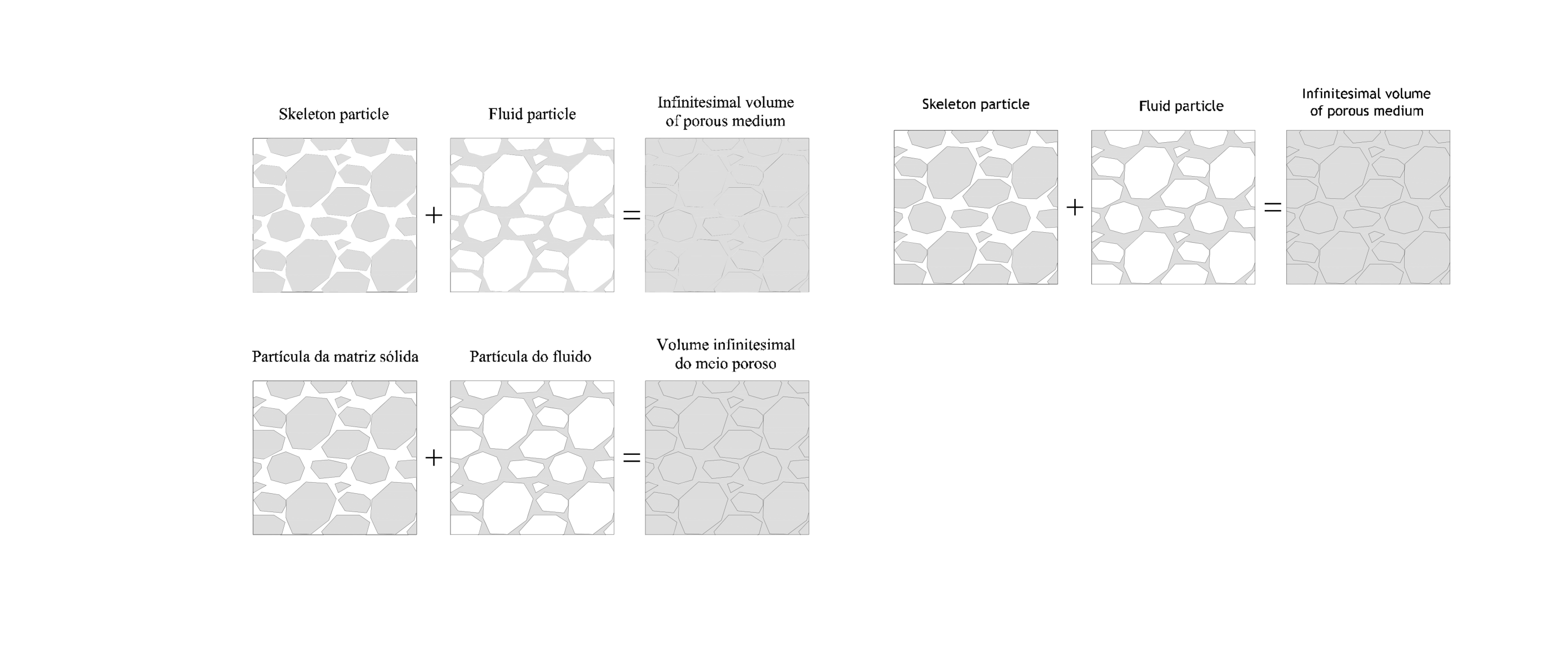
Figure 1: Fully saturated porous media (From PoromechanicsCoussy )

The proposed strategy is comprised of the following steps:

1. Particle size generation:

   1. A granulometric curve and the porosity are used as input (section 2.1).

   2. A histogram is derived from this curve, and samples are drawn from the empirical distribution provided by the histogram (section 2.2).

   3. The samples are used to estimate the parameters of a set of distributions (section 2.3).

   4. The estimated distribution that best fits the original data is adopted (section 2.4).

   5. An approximate number of particles that provide the desired porosity is calculated (section 2.5).

   6. The radii of the particles are samples of independent identically distributed random variables obeying the adopted distribution (section 2.6).

2. The particles are placed by a Simple Sequential Inhibition – SSI process on the arbitrary closed region (section 2.7). The number of particles is determined iteratively as to produce an approximation of the desired porosity.

The result of these steps is a plausible model of particle distribution in granular media, obtained with low computational cost due to its geometric nature. Algorithm 1 presents, in pseudocode, an efficient implementation of this procedure. We show that this procedure is able to simulate soils of low porosity, which are usually obtained by dynamical techniques that are much more time consuming. Such models can be used as input data for numerical simulations of problems with discontinuous media using the discrete element method.

The SSI process we employ can be seen as a RSA process with the following characteristics: the particles only interact by exclusion in a compact planar domain, i.e., there is neither attraction nor repulsion, no order is introduced in the process, i.e., the final state is jammed, particles arrive sequentially and there is no relaxation, i.e., the $(k+1)$th particle enters the sample only if the $k$th particle does.

This paper unfolds as follows. Section 2 presents the methodology of each stage of our proposal, including pseudocode algorithms. Section 3 discusses the main results, while section 4 presents the conclusions and future venues of research.

2 Particle size analysis and generation

2.1 Granulometric curve and porosity

A granulometric curve measures the percentage of the sample that falls into pre-established ranges of grain sizes. This information is obtained by seiving and hydrometer analyses, for instance. The results of such measures is provided in tabular form: $(d_{i},c_{i})_{1\leq i\leq D}$, being $c_{i}$ the (cumulative) proportion of particles whose diameter is less than $d_{i}$, and $D$ the number of diameters considered.

The porosity $\eta\in[0,1]$ is the ratio between the empty space in the sample to the total sample volume. It is estimated through the determination of the bulk density of the porous sample, then determining the density of the skeletal material, and finally correlating density and volume.

The granulometric curve and the porosity are the only required input for the rest of the methodology.

2.2 Histograms

The granulometric curve is used to form a tractable and expressive histogram of particle sizes. As presented in Figure 2, the diameters are not evenly spaced and, thus, the intervals are not equal. Such unevenness is alleviated in the semilogarithmic scale, so our proposal uses such transformation.

Consider the original data $(d_{i},c_{i})_{1\leq i\leq D}$ and its representation in semilogarithmic scale $(\ell_{i},c_{i})_{1\leq i\leq D}$, where $\ell_{i}=\log d_{i}$ for every $1\leq i\leq D$. The log-histogram of the data can be formed with the midpoints of pairs of contiguous log-diameters and the corresponding proportion of particles, i.e., $(m_{i},p_{i})_{1\leq i\leq D-1}$, where $m_{i}=(\ell_{i+1}+\ell_{i})/2$ and $p_{i}=c_{i+1}-c_{i}$. These log-histograms will be used to obtain more data from pseudorandom sampling, in order to obtain parametric models for the data.

Each dataset is, therefore, transformed into a log-histogram. Instead of using the pairs $(m_{i},p_{i})_{1\leq i\leq D-1}$, we draw $N_{i}$ independent identically distributed samples from the Uniform distribution on $(\ell_{i},\ell_{i+1})$, with $N_{i}=[kp_{i}]$ and $k$ a convenient number, for instance $k=1000$. With this, we end with $\sum_{i=1}^{D-1}N_{i}=M$ pseudorandom diameters $\bm{d}=(d_{1},\dots,d_{M})$ which, if given as input, would produce the original granulometric curve $(d_{i},c_{i})_{1\leq i\leq D}$. In this way, an arbitrary number of samples can be obtained from a single granulometric curve, leading to very precise parameter estimation.

These data $\bm{d}$ will be then used for computing estimates of parametric models able to describe the original data.

2.3 Models

2.3.1 Hyperbolic distribution

The unidimensional hyperbolic distribution is a continuous probability law characterized by the fact that the logarithm of the probability density function is a hyperbola. It was introduced by Barndorff-Nielsen1977 as a model for the log-size distribution of sand, based on the studies of Bagnold1941 about aeolian sand deposits.

This distribution and its multidimensional extensions have many applications in a variety of fields: geology, astronomy, fluid mechanics and economics Bagnold1980 ; Barndorff-Nielsen1978 ; Barndorff-Nielsen1981a ; Barndorff-Nielsen1985 , to name a few.

One of the representations of the probability density function, presented in Barndorff-Nielsen1983 , is:

$$f(x;\alpha,\beta,\mu,\delta)=\frac{\sqrt{\alpha^{2}-\beta^{2}}\exp\{-\alpha\sqrt{\delta^{2}+(x-\mu)^{2}}+\beta(x-\mu)\}}{2\alpha\delta K_{1}(\delta\sqrt{\alpha^{2}-\beta^{2}})},$$

where $x,\mu,\beta\in\mathbbm{R}$, $\delta,\alpha\in{\mathbbm{R}_{+}}$ such that $0\leq|\beta|<\alpha$, and $K_{i}$, $i=1,2,3$, denotes modified Bessel functions of the third kind. The location parameter $\mu$ is the abscissa of the point of intersection between the linear asymptotes of the hyperbola, while $\delta$ is the scale parameter. The two parameters $\alpha$ and $\beta$ determine the shape, being $\alpha$ resposible for the steepness and $\beta$ for the skewness. The distribution is symmetric for $\beta=0$.

If $X$ is a hyperbolic distributed variable, its expected value and mode are

$$E(X)=\mu+\frac{\delta\beta K_{2}(\delta\sqrt{\alpha^{2}-\beta^{2}})}{\sqrt{\alpha^{2}-\beta^{2}}K_{1}(\delta\sqrt{\alpha^{2}-\beta^{2}})}\text{ and }\operatorname{Mode}(X)=\mu+\frac{\delta\beta}{\sqrt{\alpha^{2}-\beta^{2}}},$$

and its variance is

$$\operatorname{Var}(X)= \frac{\delta K_{2}(\delta\sqrt{\alpha^{2}-\beta^{2}})}{\sqrt{\alpha^{2}-\beta^{2}}K_{1}(\delta\sqrt{\alpha^{2}-\beta^{2}})}+$$

$$\frac{\beta^{2}\delta^{2}}{\sqrt{\alpha^{2}-\beta^{2}}}\left(\frac{K_{3}(\delta\sqrt{\alpha^{2}-\beta^{2}})}{K_{1}(\delta\sqrt{\alpha^{2}-\beta^{2}})}-\frac{K_{2}^{2}(\delta\sqrt{\alpha^{2}-\beta^{2}})}{K_{1}^{2}(\delta\sqrt{\alpha^{2}-\beta^{2}})}\right).$$

Another representation of the density function of the hyperbolic distribution is:

$$f(x;\pi,\zeta,\mu,\delta)=\frac{\exp\Bigl{\{}-\zeta\Bigl{(}\sqrt{1+\pi^{2}}\sqrt{1+(\frac{x-\mu}{\delta})^{2}}-\pi\frac{x-\mu}{\delta}\Bigr{)}\Bigr{\}}}{2\delta\sqrt{1+\pi^{2}}K_{1}(\zeta)},$$

where $x,\mu,\pi\in\mathbbm{R}$, and $\delta,\zeta\in{\mathbbm{R}_{+}}$. The parameter $\zeta$ is a measure of the degree of peakedness, and $\pi$ is a measure of the asymmetry of the distribution. When $\pi=0$, the distribution is symmetric. Together, they determine the shape of the distribution. $\mu$ and $\delta$ are parameters of location and scale. This last parametrization is employed by the HyperbolicDist package of R ManualR , which also provides techniques for computing maximum likelihood estimates.

2.3.2 Gamma distribution

The gamma distribution is a continuous probability distribution of two parameters. It has been used in a wide range of disciplines: from climatology (in particular, to study rainfall; see Aksoy2000 ), to material analysis Basu2009 , to name a few.

It has a scale parameter $\lambda$ and a shape parameter $\alpha$, both positive, in its density function:

$$f(x;\alpha,\lambda)=\frac{x^{\alpha-1}e^{-{x}/{\lambda}}}{\lambda^{\alpha}\Gamma(\alpha)}{\mathbbm{1}}_{\mathbbm{R}_{+}}(x),$$

where $\Gamma$ is the incomplete gamma function given by $\Gamma(\alpha)=\int_{0}^{\infty}x^{\alpha-1}e^{-x}dx$. Alternatively, it can be parameterized in terms of the rate $\beta={1}/{\lambda}$.

If $X$ is a gamma distributed variable, its expected value, mode and variance are:

$$E(X)=\alpha\lambda,\quad\text{Mode}(X)=(\alpha-1)\lambda,\text{ and}\quad\text{Var}(X)=\alpha\lambda^{2},$$

respectively.

2.3.3 Lognormal distribution

The lognormal distribution is the distribution of any random variable whose logarithm is normally distributed. It is widely used in physics, statistics, geology, economics, biology etc. Its probability density function is

$$f(x;\mu,\sigma)=\frac{1}{x\sigma\sqrt{2\pi}}\exp\Bigl{\{}-\frac{(\ln{x}-\mu)^{2}}{2\sigma^{2}}\Bigr{\}}{\mathbbm{1}}_{\mathbbm{R}_{+}}(x),$$

where $\mu\in\mathbbm{R}$ and $\sigma>0$.

If $X$ is a lognormally distributed variable, its expected value, mode and variance are

$$E(X)=e^{\mu+{\sigma^{2}}/{2}},\quad\text{Mode}(X)=e^{\mu-\sigma^{2}},\text{ and}\quad\text{Var}(X)=(e^{\sigma^{2}}-1)e^{2\mu+\sigma^{2}},$$

respectively.

2.3.4 Weibull distribution

This law is often called the Rosin-Rammler distribution when used to describe the size distribution of particles Rosin1933 . The probability density function of a Weibull random variable $X$ is

$$f(x;\alpha,\lambda)=\alpha{\lambda^{\alpha}}{x^{\alpha-1}}e^{-(\lambda x)^{\alpha}}{\mathbbm{1}}_{\mathbbm{R}_{+}}(x),$$

where $\alpha,\lambda>0$ are the shape and the scale parameters, respectively.

If $X$ is a Weibull distributed variable, its expected value, mode and variance are:

$$E(X)=\lambda\Gamma\Bigl{(}1+\frac{1}{\alpha}\Bigr{)},\quad\text{Mode}(X)=\lambda\Bigl{(}\frac{\alpha-1}{\alpha}\Bigr{)}^{\frac{1}{\alpha}},$$

and

$$\text{Var}(X)=\frac{1}{\lambda^{2}}\Bigl{(}\Gamma\bigl{(}\frac{\alpha+2}{\alpha}\bigr{)}-\Gamma^{2}\bigl{(}\frac{\alpha+1}{\alpha}\bigr{)}\Bigr{)},$$

respectively.

2.4 Choice of the best model

Each sample is used to estimate the maximum likelihood parameters $\widehat{\theta}$ that index the four distributions $\mathcal{D}$ considered as candidate models, and then the $\chi^{2}$ goodness-of-fit test is applied. In principle, the model with highest $p$-value should be chosen as the best statistical description and, in case of tiers, the one with least computational requirements should be the final choice.

Other goodness-of-fit test as, for instance, the Kolmogorov-Smirnov test, can be used, as well as other estimation procedures, e.g., moment or analogy estimators.

2.5 Number of particles

We will derive an initial guess for the number of particles to be generated in order to have a good approximation of the desired prosity.

Assume the closed area of interest, $W$, has size $\mu(W)$, which we want to fill with particles whose radii follow the parametric model $\mathcal{D}(\widehat{\theta})$ chosen as previously discussed. We also have the desired porosity $\eta$, estimated from the soil sample:

$$\eta=\frac{V_{e}}{\mu(W)}=\frac{\mu(W)-V_{p}}{\mu(W)},$$

where $V_{e}$ and $V_{p}$ are the empty and particles areas, respectively. The area of a disk with radius $R$, distributed according to the law $\mathcal{D}(\widehat{\theta})$ is a random variable given by $V=\pi R^{2}$. Then, assuming that $N$ particles are placed within $W$,

$$V_{p}=\pi\sum_{i=1}^{N}R_{i}^{2}.$$

Using expected values,

$$\operatorname{E}(V_{p})=\pi\sum_{i=1}^{N}\operatorname{E}(R_{i}^{2})=\pi\sum_{i=1}^{N}[\operatorname{Var}(R_{i})+\operatorname{E}^{2}(R_{i})]=N\pi[\operatorname{Var}(R_{i})+\operatorname{E}^{2}(R_{i})],$$

and both variance and expected value are given explicitely as functions of the estimated parameter $\widehat{\theta}$, so

$$N=\frac{(1-\eta)\mu(W)}{\pi[\widehat{\operatorname{Var}}(R_{i})+\widehat{\operatorname{E}}^{2}(R_{i})]}.$$

This number of particles $N$ is intended as a rough estimate of the needed number of radii required to fill $W$ with the desired porosity and granulometry.

2.6 Generation of particles

Four distributions are considered in this work, namely the Hyperbolic, Gamma, Log-normal and Weibull laws. Sampling from the two first requires specialized algorithms, samples from the third are the exponential transformation of normal deviates, and inversion is required in order to sample from the last one. All these samples are produced calling functions available in the R platform Crawley2007 .

Algorithm 1 presents, in pseudocode, a sequential approach for obtaining a good approximation to the desired porosity $\eta$, while keeping the statistical properties of the particles. In this algorithm, $K>1$ is a factor which controls the number of extra particles to be generated; we set $K=10$, a good compromise between the relatively low cost of generating outcomes versus the high cost of initializing the generator.

Algorithm 1 Sequential sampling of radii for a desired porosity

1:procedure SequentialRadii($W$, $N$, $\eta$, $\mathcal{D}(\widehat{\theta})$, $K$) $\triangleright$ Region of interest, number of particles, porosity, model and factor

2:     Obtain $\bm{r}=(r_{1},\dots,r_{KN})$ samples from independent identically distributed random variables following the $\mathcal{D}(\widehat{\theta})$ distribution

3:     Allocate the vector of coordinates $\bm{c}=((x_{1},y_{1}),\dots,(x_{KN},y_{KN}))$

4:     $i\leftarrow 0$, $\eta_{i}\leftarrow 1$ $\triangleright$ Initialize counter and porosity

5:     while $\eta_{i}>\eta$ do

6:         condition $\leftarrow\textrm{SSI}(W,i,\bm{r},\bm{c})$ $\triangleright$ Defined on Algorithm 2

7:         if condition = TRUE then

8:              $i\leftarrow i+1$ $\triangleright$ Update counter

9:              $\eta_{i}\leftarrow\eta_{i-1}-\pi r_{i}^{2}/\mu(W)$ $\triangleright$ Update porosity

10:         else

11:              break $\triangleright$ No more particles will be placed

12:         end if

13:     end while

14:     if $i=0$ then

15:         return FAIL $\triangleright$ The first particle could not be placed in $W$

16:     else

17:         return $((x_{1},y_{1},r_{1}),\dots,(x_{i},y_{i},r_{i}),\eta_{i})$ $\triangleright$ Returns coordinates, radii and current porosity

18:     end if

19:end procedure

This algorithm places a number of particles obeying the $\mathcal{D}(\widehat{\theta})$ distribution which approximates the desired porosity $\eta$ on the region of interest $W$.

It is noteworthy that the presented methodology can be immediately extended to compact volumes.

2.7 Spatial distribution by the SSI process

Line 6 of Algorithm 1 makes a call to the procedure presented in Algorithm 2, which implements the sampling from the simple sequential inhibition point processes. Such processes are defined in terms of a window $W$, the number of points and the exclusion radii among them BerthelsenMoller:PrimerSPP:2002 ; in our case, the number of points is, instead of specified a priori, controlled by the desired porosity $\eta$ on $W$.

The Simple Sequential Inhibition (SSI) point process for $n$ points on $W$ with exclusion radii $\bm{r}=(r_{1},\dots,r_{n})$ and maximum number of iterations $j_{\max}$ tries to place $n$ non-overlapping disks of radii $\bm{r}$ by testing sequentially each disk against the previous ones. The first disk is placed uniformly on $W$, provided it does not surpass the boudaries. Subsequent steps sample a point in $W$ uniformly and independently of previous disks, and verifies if there is no overlapping; if there is not, the disk is placed, otherwise up to $j_{\max}$ independent trials are made. The algorithm stops when all the disks have been placed, or when the maximum number of iterations has been reached, whichever takes place first. Our implementation of the SSI point process is presented in Algorithm 2.

Algorithm 2 Simple sequential inhibition point process

1:procedure SSI($W,i,\bm{r},\bm{c}$) $\triangleright$ Region of interest, iteration, radii and coordinates

2:     Define $j_{\max}$ $\triangleright$ The maximum number of trials per particle

3:     $j\leftarrow 0$

4:     while $j<j_{\max}$ do

5:         Sample $(x,y)$ uniformly on $W$

6:         if $\min_{1\leq k<i}\{d((x,y),(x_{k},y_{k}))\geq r_{i}\}$ then

7:              $c(i)\leftarrow(x,y)$ $\triangleright$ Place particle $i$ at $(x,y)$

8:              return TRUE $\triangleright$ Success

9:         else

10:              $j\leftarrow j+1$

11:         end if

12:     end while

13:     return FALSE $\triangleright$ Unable to place the $i$-th particle

14:end procedure

Notice that the order in which the particles are places is not altered. In particular, if particle $i\leq 2$ does not fit after $j_{\max}$ trials, the algorithm returns the current state which consists of the previous $i-1$ particles. Even if particle $i+1$ fits trivially the current state, it is not included. Selecting particles by their size would imply independent identically distributed random variables model, and switching to a collection of correlated deviates: the order statistics.

Dense samples are, typically, harder to obtain than situations of high porosity. In those cases it is likely that the denser the desired outcome the more results will have to be discarded until a sample with the desired property is obtained.

3 Results

This section presents results related to the two main steps already discussed, namely, particle size generation and placement. The example used to illustrate this work is based on collected disturbed samples from the Barreiras formation and other fluvial deposits in Alagoas state, Brazil, in order to study their granulometric properties.

The granulometric information is obtained in tabular form: $(d_{i},c_{i})_{1\leq i\leq D}$, being $c_{i}$ the (cumulative) proportion of particles whose diameter is less than $d_{i}$, and $D$ the number of diameters considered.

The samples used as input for this analysis are presented in Table 1. Figure 2 presents the result of the sieving process applied to Sample 1. The table shows the diameters, in decreasing order and in mm, and the corresponding cumulative percentage of passing particles. This same information is shown in the form of a granulometric curve in linear scale (right top); the sieves diameters are show superimposed to the abscissa axis. The clutter effect of small sieves is evident, therefore the frequent choice of presenting such curves in semilogarithmic scale (right bottom). Notice that the diameters are not evenly distributed deserving, thus, a careful treatment.

Table 1: Soil types analized

Sample	Soil type	Porosity $\eta$
1	sand, silt with traces of de gravel	0.35
2	sand with traces of silt	0.43
3	sand, portions of clay, traces of silt and gravel	0.42
4	sand with traces of silt	0.39
5	sandy clay with portions of silt	0.40
6	sandy clay with portions of silt and traces of gravel	0.33
7	sand	0.44

Diameter [mm]	Cumulative %
4.800	100.00
2.000	98.65
1.200	83.81
0.840	70.66
0.710	61.49
0.600	56.29
0.500	46.38
0.420	42.16
0.350	36.41
0.297	30.50
0.250	28.30
0.210	25.85
0.177	22.58
0.149	20.49
0.105	16.39
0.088	15.53
0.075	14.86
0.050	8.34
0.036	8.34
0.025	6.95
0.017	6.25
0.013	6.25
0.009	3.46
0.006	2.76
0.005	1.92
0.003	1.09
0.002	0.00

(a) Original granulometric curve

(b) Granulometric curve in semilogarithmic scale

Figure 2: Granulometric data and curves: linear (a, top) and semilogarithmic (b, bottom), sample 1

Each data set from Table 1 was analyzed using the procedure presented in previous sections, i.e., (i) its granulometric curve was obtained by sieving (see Figure 2 as an example), (ii) a histogram was formed (Figures 3 and 4), (iii) samples of pseudorandom diameters were drawn. These diameters were then analyzed by fitting the gamma, lognormal, Weibull and hyperbolic distributions. Maximum likelihood estimation was performed using the fitdistr function from the MASS package of R (for the gamma, lognormal and Weibull distribution) and the hyperbFit function from the HyperbolicDist package (for the hyperbolic distribution). The estimated parameters, rounded to the third decimal place, are given in Table 2.

Table 2: Estimated parameters

Sample	Gamma		Lognormal		Weibull		Hyperbolic
	$\widehat{\alpha}$	$\widehat{\beta}$	$\widehat{\mu}$	$\widehat{\sigma}$	$\widehat{\alpha}$	$\widehat{\lambda}$	$\widehat{\pi}$	$\widehat{\zeta}$	$\widehat{\delta}$	$\widehat{\mu}$
1	$43.717$	$4.170$	$2.338$	$0.159$	$10.281$	$11.046$	$-1.055$	$0.750$	$0.403$	$11.892$
2	$342.999$	$32.155$	$2.366$	$0.054$	$18.806$	$10.943$	$0.235$	$15.073$	$2.072$	$10.132$
3	$81.896$	$7.437$	$2.393$	$0.113$	$11.241$	$11.513$	$-3.369$	$19.473$	$1.367$	$15.977$
4	$387.377$	$36.738$	$2.354$	$0.051$	$21.186$	$10.799$	$-0.138$	$705.286$	$14.081$	$12.495$
5	$114.429$	$11.722$	$2.274$	$0.095$	$12.564$	$10.163$	$-1.171$	$45.259$	$3.816$	$14.381$
6	$90.818$	$9.153$	$2.289$	$0.106$	$10.231$	$10.381$	$0.107$	$2.635$	$1.304$	$9.698$
7	$334.601$	$130.210$	$2.403$	$0.055$	$16.146$	$11.372$	$0.159$	$2.025$	$0.631$	$10.895$

The $p$-values of the $\chi^{2}$ test were computed, and they all resulted above $0.99$ with one exception, the Weibull distribution for sample 7. Therefore, for the samples here analyzed, the choice of the “best” model can be guided by the computational cost of producing pseudorandom deviates or by any other criterion.

We simulated samples from each of the types of soil previously analized using the models presented in Table 3, which describe the logarithm of the diameters. These simulations were performed in squared boxes specifying the desired porosity. Table 3 also presents the number of particles generated in each case ($N$), along with the desired and obtained porosities ($\eta$ and $\widehat{\eta}$, respectively). Given the similarity of the results, in Figure 5 we only present the simulation corresponding to Sample 6. Figure 5(a) presents the $34688$ particles that were generated to fill a box with the specified porosity, while Figure 5(b) shows a detail where both the varibility of the model and the non-overlapping results are enhanced.

Figure 3: Loghistogram and fitted density for sample 1

(a) Sample 2

(b) Sample 3

(c) Sample 4

(d) Sample 5

(e) Sample 6

(f) Sample 7

Figure 4: Loghistograms and fitted densities

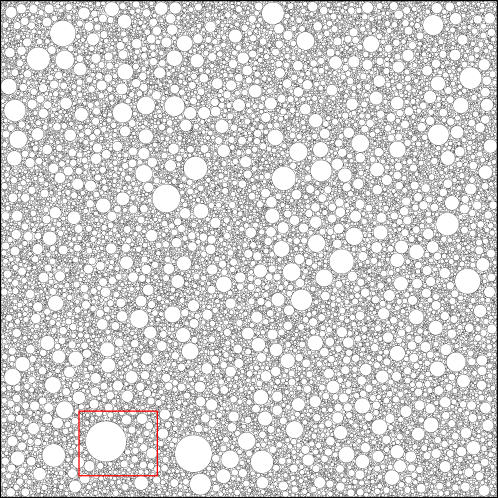
(a) Complete simulation

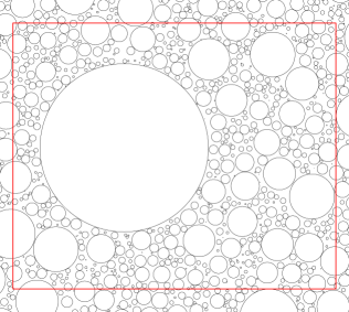
(b) Detail

Figure 5: Simulated soil from Sample 6

Table 3: Chosen model for each sample, number of particles, desired and obtained porosities

Sample	$\mathcal{D}$	$N$	$\eta$	$\widehat{\eta}$
1	Weibull	$6704$	$0.350$	$0.345$
2	Hyperbolic	$4846$	$0.430$	$0.421$
3	Gamma	$1922$	$0.420$	$0.418$
4	Lognormal	$7840$	$0.390$	$0.390$
5	Weibull	$27486$	$0.400$	$0.399$
6	Weibull	$34688$	$0.330$	$0.328$
7	Hyperbolic	$1611$	$0.440$	$0.430$

4 Conclusions and future work

We proposed and assessed a fast geometric algorithm which produces spatially homogeneous samples with specified porosity and granulometric curve using disks. Starting with the granulometric curve and porosity of a soil, our algorithm produces samples of any size in closed arbitrary domains. The outcomes of this algorithm can be used as granular media samples in computational simulations, e.g., discrete elements.

The algorithm allows the use of any suitable distribution for the particle size. It was assessed with seven samples and four distributions, and in every case it produced samples wich mimic well the input data.

The proposed strategy can also be used in the simulation of other physical systems. Kadau et al. Kadau2009 propose a two‐dimensional contact dynamics model as a microscopic description of a collapsing suspension/soil to capture the essential physical processes underlying the dynamics of generation and collapse of the system. Kadau and Herrmann Kadau2011 study the influence of the granular Bond number on the density profiles and the generation process of packings, generated by ballistic deposition under gravity. Both works deal with loose granular media and, thus, there is no need to impose strong physical constraints.

The research continues with the proposal of a hybrid technique which, starting with our geometrical algorithm, produces a final configuration in geostatic equilibrium by relaxation in both 2D and 3D domains.

- (1) Aksoy, H.: Use of gamma distribution in hydrological analysis. Turkish Journal of Engineering and Environmental Sciences 24, 419–428 (2000)
- (2) Bagi, K.: An algorithm to generate random dense arrangements for discrete element simulations of granular assemblies. Granular Matter 7, 31–43 (2005)
- (3) Bagnold, R.A.: The physics of blown sands and desert dunes, second edn. Chapman and Hall (1941). London: Methuel
- (4) Bagnold, R.A., Barndorff-Nielsen, O.: The pattern of natural size distributions. Sedimentology 27(2), 199–207 (1980). DOI 10.1111/j.1365-3091.1980.tb01170.x
- (5) Barndorff-Nielsen, O.E.: Exponentially decreasing distributions for logarithm of particle-size. Proceedings of the Royal Society of London Series A: Mathematical Physical and Engineering Sciences 353(1674), 401–419 (1977)
- (6) Barndorff-Nielsen, O.E.: Hyperbolic distribution and distribution on hyperbolae. Scandinavian Journal of Statistics 5, 151–157 (1978)
- (7) Barndorff-Nielsen, O.E., Blaesild, P.: Hyperbolic distributions and ramifications: contributions to theory and application, vol. 4, pp. 19–44. Reidel Publishing Company (1981)
- (8) Barndorff-Nielsen, O.E., Blaesild, P.: Hyperbolic distributions. In: Encyclopedia of statistical sciences, vol. 3. Wiley (1983)
- (9) Barndorff-Nielsen, O.E., Blaesild, P., Jensen, J.L., Sorensen, M.: The fascination of sand. In: A.C. Atkinson, S.E. Fienberg (eds.) A celebration of statistics: The International Statistical Institute ISI centenary volume, vol. Centenary volume of the International Statistical Institute, chap. 4, pp. 57–87. Springer Verlag (1985)
- (10) Basu, B., Tiwari, D., Kundu, D., Prasad, R.: Is Weibull distribution the most appropriate statistical strength distribution for brittle materials? Ceramics International 35(1), 237–246 (2009). DOI http://dx.doi.org/10.1016/j.ceramint.2007.10.003
- (11) Berthelsen, K.K., Møller, J.: A primer on perfect simulation for spatial point processes. Bulletin of the Brazilian Mathematical Society 33(3), 351–367 (2002). DOI 10.1007/s005740200019
- (12) Bittelli, M., Campbell, G.S., Flury, M.: Characterization of particle-size distribution in soils with a fragmentation model. Soil Science Society of America Journal 63(4), 782–788 (1999)
- (13) Buchan, G.D., Grewal, K.S., Robson, A.B.: Applicability of the simple lognormal model to particle-size distribution in soils. Soil Science 147, 155–161 (1989)
- (14) Buchan, G.D., Grewal, K.S., Robson, A.B.: Improved models of particle-size distribution – An illustration of model comparison techniques. Soil Science Society of America Journal 57(4), 901–908 (1993)
- (15) Cadilhe, A., Araújo, N.A.M., Privman, V.: Random sequential adsorption: from continuum to lattice and pre-patterned substrates. Journal of Physics: Condensed Matter 19, 065,124 (12pp) (2007)
- (16) Coussy, O.: Poromechanics. John Wiley & Sons, Chichester (2004)
- (17) Crawley, M.J.: The R book. Wiley (2007)
- (18) Cui, L., O’Sullivan, C.: Analysis of a triangulation based approach for specimen generation for discrete element simulation. Granular Matter 5, 135––145 (2003)
- (19) Cundall, P.A.: Formulation of a three dimensional distinct element model-part I: A scheme to detect and represent contacts in a system of many polyhedral blocks. International Journal of Rock Mechanics, Mining Sciences and Geomechanics Abstracts 25(3), 107–116 (1988)
- (20) Cundall, P.A., Strack, O.D.L.: A discrete numerical method for granular assemblies. Geotechnique 29, 47–65 (1979)
- (21) da Silva, E.M., Lima, J.E.F.W., Rodrigues, L.N., de Azevedo, J.A.: Comparison of mathematical models for fitting particle-size distribution curves. Pesquisa Agropecuaria Brasileira 39(4), 363–370 (2004)
- (22) Eshel, G., Levy, G.J., Mingelgrin, U., Singer, M.J.: Critical evaluation of the use of laser diffraction for particle-size distribution analysis. Soil Science Society of America Journal 68(3), 736–743 (2004)
- (23) Feng, Y.T., Han, K., R., O.D.: Filling domains with disks: an advancing front approach. Methods in Engineering 56(5), 699–731 (2003)
- (24) Fieller, N.R.J., Flenley, E.C.: Statistics of particle size data. Applied Statistics 41(1), 127–146 (1992)
- (25) Fisher, R.A., Odén, S.: The theory of the mechanical analysis of sediments by means of the automatic balance. Proceedings of The Royal Society of Edinburgh 44, 98–115 (1923)
- (26) Fredlund, M.D., Fredlund, D.G., Wilson, G.W.: An equation to represent grain-size distribution. Canadian Geotechnical Journal 37(4), 817–827 (2000)
- (27) Hwang, S.I., Lee, K.P., Lee, D.S., Powers, S.E.: Models for estimating soil particle-size distributions. Soil Science Society of America Journal 66(4), 1143–1150 (2002)
- (28) Itasca, Minneapolis, MN: PFC2D 2.00 Particule Flow Code in Two Dimensions (1998)
- (29) Kadau, D., Herrmann, H.J.: Density profiles of loose and collapsed cohesive granular structures generated by ballistic deposition. Physical Review E 83 (2011)
- (30) Kadau, D., Herrmann, H.J., Andrade Jr., J.S.: Collapsing granular suspensions. The European Physical Journal E: Soft Matter and Biologycal Physics 30, 275–281 (2009)
- (31) Labra, C., Oñate, E.: High-density sphere packing to discrete element method simulations. Communications in Numerical Methods in Engineering (2008)
- (32) Lin, X., Ng, T.T.: A three-dimensional discrete element model using arrays of ellipsoids. Geotechnique 47(2), 319––329 (1997)
- (33) Lohner, R., Oñate, E.: A general advancing front technique for filling space with arbitrary objects. International Journal for Numerical Methods in Engineering 61, 1977––1991 (2004)
- (34) Mallows, C.L.: Some comments on Cp. Technometrics 15, 661–675 (1973)
- (35) Martin, M.A., Taguas, F.J.: Fractal modelling, characterization and simulation of particle-size distributions in soil. Proceedings of The Royal Society of London Series A: Mathematical Physical and Engineering Sciences 454(1973), 1457–1468 (1998)
- (36) Morgan, P.H., Mercer, L.P., Flodin, N.W.: General model for nutritional responses of higher organisms. Proceedings of the National Academy of Sciences 42, 4327–4331 (1975)
- (37) Nemes, A., Wösten, J.H.M., Lilly, A., Voshaar, J.H.O.: Evaluation of different procedures to interpolate particle-size distributions to achieve compatibility within soil databases. Geoderma 90, 187–202 (1999)
- (38) Privman, V.: Dynamics of nonequilibrium deposition. Colloids and Surfaces A: Physicochemical and Engineering Aspects 165, 231–240 (2000)
- (39) R Development Core Team: R: A Language and Environment for Statistical Computing. R Foundation for Statistical Computing, Vienna, Austria (2010). URL http://www.R-project.org. ISBN 3-900051-07-0
- (40) Rosin, P., Rammler, E.: The laws governing the fineness of powdered coal. Journal of the Institute of Fuel 7, 29–36 (1933)
- (41) Rousseva, S.S.: Data transformations between soil texture schemes. European Journal of Soil Science 48, 749–758 (1997)
- (42) Shiozawa, S., Campbell, G.S.: On the calculation of mean particle diameter and standard deviation from sand, silt and clay fractions. Soil Science 152, 427–431 (1991)
- (43) Shirazi, M.A., Boersma, L.: A unifying quantitative analysis of soil texture. Soil Science Society of American Journal 48, 142–147 (1984)
- (44) Skaggs, T.H., Arya, L.M., Shouse, P.J., Mohanty, B.P.: Estimating particle-size distribution from limited soil texture data. Soil Science Society of America Journal 65(4), 1038–1044 (2001)
- (45) Walker, P.H., Chittleborough, D.J.: Development of particle-size distributions in some alfisols of Southeastern Australia. Soil Science Society of American Journal 50, 394–400 (1986)
- (46) Weibull, W.A.: A statistical distribution function of wide applicability. Journal of Applied Mechanics 73, 293–297 (1951)
- (47) Zarate, F., Rojek, J., Oñate, E., Miquel, J.: Modelling of rock, soil and granular materials using spherical elements. In: Z. Waszczyszyn, J. Pamin (eds.) ECCM-2001 CD-ROM Proceedings of the Second European Conference on Computational Mechanics: Solids, Structures and Coupled Problems in Engineering. Cracow (2001)
- (48) Zarate, F., Rojek, J., Oñate, E., Miquel, J.: Thermomechanical discrete element formulation for wear analysis of rock cutting tools. Tech. rep., CIMNE (2004)