An interface phase transition induced by a driven line in 2D

Abstract

The effect of a localized drive on the steady state of an interface separating two phases in coexistence is studied. This is done using a spin conserving kinetic Ising model on a two dimensional lattice with cylindrical boundary conditions, where a drive is applied along a single ring on which the interface separating the two phases is centered. The drive is found to induce an interface spontaneous symmetry breaking whereby the magnetization of the driven ring becomes non-zero. The width of the interface becomes finite and its fluctuations around the driven ring are non-symmetric. The dynamical origin of these properties is analyzed in an adiabatic limit which allows the evaluation of the large deviation function of the driven-ring magnetization.

The effect of local drive on the properties of an interface separating two coexisting phases has recently been explored as a simple example of systems driven away from equilibrium. Much of the attention is due to the surprising experimental results on colloidal gas-liquid interface subjected to a shear flow parallel to the interface DERKS . It was found that the shear drive applied away from the interface, strongly suppresses the fluctuations of the interface, making it smoother. This long-distance effect of the drive is due to long-range correlations that characterize driven systems SMM ; KLS1 ; *KLS2; SPOHN ; ZHANG ; GARRIDO ; RUBI ; ZIA . An interesting theoretical approach for studying this phenomenon has been introduced by Smith et al. who considered a two dimensional version of the system, and modeled it by an Ising lattice-gas below its transition temperature SMITH . Using spin conserving Kawasaki dynamics and applying shear flow at the boundaries parallel to the interface, it was observed that the interface indeed becomes narrower although its width still increases with the length of the interface. In closely related works, the effect induced by a current carrying line on a neighboring non-driven one has also been analyzed DICKMAN ; KOLOMEISKY ; HUCHT ; HILHORST .

In this Letter we consider a drive localized along an interface which separates two coexisting phases, and study the resulting interface properties. This is done using a two dimensional Ising model on a square lattice with cylindrical boundary conditions (Fig. 1), that evolves under spin conserving dynamics. The drive acts along the ring around which the interface is centered. We find that the drive induces an interface phase transition which involves spontaneous symmetry breaking, resulting in a non-zero magnetization of the driven ring. In this transition, the macroscopic $2D$ steady state remains unchanged, however spontaneous symmetry breaking takes place involving the steady state of a $1D$ stripe centered on the driven ring. This is in sharp contrast with an equilibrium setup of an interface subjected to a localizing potential along a ring, where the ring magnetization vanishes at all temperatures, and no interface spontaneous symmetry breaking takes place. Moreover, we find that the drive suppresses the fluctuations of the interface, leading to an interface with a finite width which does not scale with the system size. Also, due to the broken symmetry on the driven ring, the interface fluctuations are highly asymmetric. The interface fluctuates more strongly into the bulk phase whose magnetization is opposite to that of the driven ring. These results are first demonstrated by numerical simulations. The model is then analyzed in a special limit which allows analytical computation of the large deviation function (LDF) TOUCHETTE of the magnetization of the driven ring, demonstrating the existence of the spontaneous symmetry breaking.

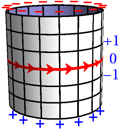
Figure 1: (color online) Square lattice with cylindrical boundary condition, with the drive on the central ring and the boundary conditions indicated.

To proceed, we consider Ising spins $\boldsymbol{\sigma}\equiv\left\{\sigma_{\mathbf{r}}\right\}$ on sites $\mathbf{r}=(x,y)$ of an $L\times(2M+1)$ square lattice, with periodic boundary condition in the x-direction while the two open boundaries, $y=\pm M$, are coupled to rows from above ($y=M+1$) and below ($y=-M-1$), respectively, with fixed spins: $\sigma_{x,\pm M\pm 1}=\mp 1$ (Fig. 1). The model has nearest neighbor ferromagnetic interactions and a drive is introduced by a force field $\mathbf{E}\equiv(E,0)$ applied on the $y=0$ ring. The field favors the positive spins to move counter clockwise along the ring, and as a result drives the system out of equilibrium.

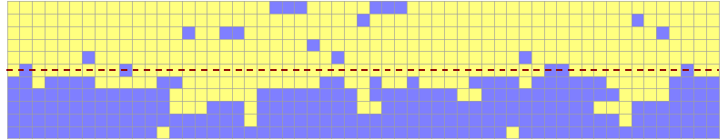
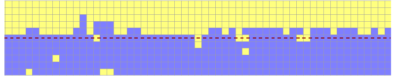
Figure 2: (color online) Typical spin configurations zoomed around the driven ring (denoted by a dashed line) for $L=2M=100$ at $T=0.85T_{c}$. Blue (dark) and yellow (light) squares indicate $+$ and $-$ spins, respectively.

There is more than one way to incorporate the drive in the dynamics, and unlike a dynamics satisfying detailed balance, the steady state depends on the precise choice of the rates KWAK . We choose a modified Metropolis algorithm KLS1 where in every step a pair of nearest neighbor sites $\mathbf{r}$ and $\mathbf{r^{\prime}}$ are chosen at random and their spins are exchanged with probability $\rm{min}\{1,\exp(-\beta\Delta\mathcal{H})\}$, where $\beta$ is an inverse temperature and $\Delta\mathcal{H}$ is the energy difference between the final and initial configurations. Thus, for exchanging $\sigma_{\mathbf{r}}$ and $\sigma_{\mathbf{r^{\prime}}}$,

$$\Delta\mathcal{H}=\begin{cases}\Delta H-(\sigma_{\mathbf{r}}-\sigma_{\mathbf{r^{\prime}}})(\mathbf{r^{\prime}}-\mathbf{r})\cdot\mathbf{E}&\text{if $\mathbf{r}$,$\mathbf{r^{\prime}\in}$ $0$th ring,}\\ \Delta H&\text{elsewhere,}\end{cases}$$

where $\Delta H$ is calculated using the Ising Hamiltonian $H=-J\sum_{\langle\mathbf{r},\mathbf{r^{\prime}}\rangle}\sigma_{\mathbf{r}}\sigma_{\mathbf{r^{\prime}}}$, with $J>0$. One Monte Carlo time step is constituted of $L(4M+1)$ such updates. In all the numerical results presented in this Letter we use a large driving field $E\geq 10J$.

In absence of a driving field, the model is in equilibrium. At sub-critical temperatures ($T<T_{c}\simeq 2.2692J/k_{B})$, the equilibrium state is composed of two oppositely magnetized phases, separated by an interface. For an initial configuration with zero overall magnetization, the magnetization profile in the $y$ direction, $m_{y}\equiv 1/L\sum_{x}\sigma_{x,y}$, is antisymmetric with respect to $y=0$. The interface fluctuates symmetrically around the driven ring, leading to zero magnetization on the ring, $m_{0}=0$. In the large $L,M$ limit with fixed aspect ratio $L/M$, the width of the interface scales as $\sqrt{L}$ REED .

Introducing a drive does not modify the overall macroscopic structure of the steady state. As is naively expected, the steady state is still composed of two oppositely magnetized phases separated by a fluctuating interface around $y=0$. However, numerical studies of the model reveal some profound changes in the structure of the interface itself. In particular we find that (a) in the thermodynamic limit the magnetization of the driven line, $m_{0}$, is non-zero, taking one of two oppositely directed values. It thus breaks the $\sigma_{\mathbf{r}}\rightarrow-\sigma_{-\mathbf{r}}$ symmetry of the model. (b) The interface is localized around the driven line and its width stays finite in the thermodynamic limit, and (c) the fluctuations of the interface into the two bulk phases are highly asymmetric, with more pronounced fluctuations into the phase whose magnetization is oppositely directed to that of the driven line.

In Fig. 2 we present two typical microscopic configurations of the model. It is clearly seen that the driven line is predominantly occupied by either positive or negative spins representing its two possible ordered states. As the system evolves, the magnetization $m_{0}$ fluctuates around one of the non-zero values for a long time. It then switches to the oppositely magnetized state over a much shorter time scale, as shown in Fig. 3.

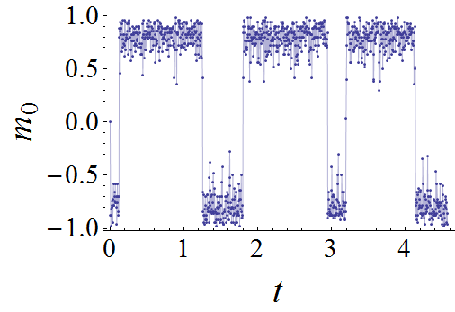
Figure 3: Typical time evolution of $m_{0}$ for $L=2M=100$ at $T=0.6T_{c}$. Time is measured in Monte Carlo steps.

The numerical result for the average time between two successive such switches, $t_{s}$, are shown in Fig. 4. The data suggest that $t_{s}$ grows exponentially with $L$, with $t_{s}\sim\exp(0.06L)$. The data for each $L$ is averaged over $n$ number of switches that are observed in available computation time ($n$ varies from around $12000$ to $10$ as $L$ changes from $30$ to $130$); $n$ decreases with $L$, yielding increasing error bars of order $1/\sqrt{n}$ with $L$. Although the range of the system size studied is insufficient for a conclusive evidence of an exponential growth, this form is justified by the theoretical results presented below. The exponential growth implies that in the thermodynamic limit, the two non-zero values of $m_{0}$ correspond to two thermodynamically stable phases.

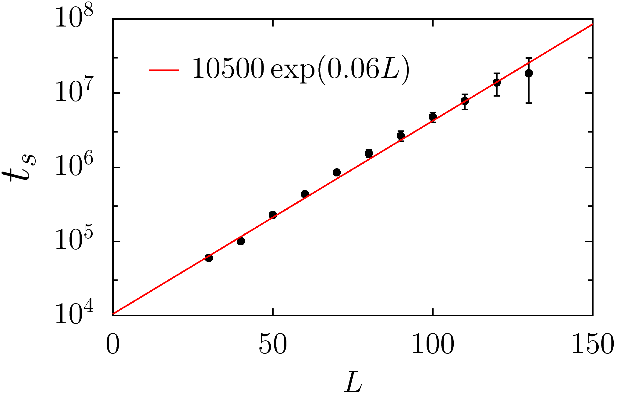
Figure 4: Average time between consecutive switches $t_{s}(L)$ for $2M=L$, and $T=0.6T_{c}$

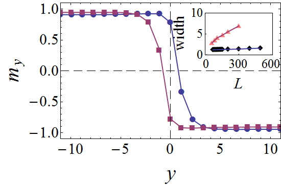
Figure 5: (color online) The average magnetization profile $m_{y}$ corresponding to the two phases, close to $y=0$. The asymmetry around $y=0$ is clearly seen. The profiles are generated on a $100\times 101$ lattice at $T=0.85T_{c}$, averaging over $10^{5}$ configurations at regular intervals of $1000$ Monte Carlo steps. The figure in the inset shows the growth of the width of the interface with increasing length $L$ for zero drive (top curve) and for driving strength $E=10J$ (lower curve).

The width of the interface is evaluated by averaging $|y|$ weighted by the derivative $dm_{y}/dy$ that peaks at the interface position. The result is shown in the inset of Fig. 5 for both driven and non-driven case. A comparison of the two cases clearly indicates that the interface fluctuations are drastically reduced in the presence of drive. As will be shown by the theoretical analysis presented below, the width of the interface remains finite at large $L$. Such smoothening of the interface has also been observed in presence of global drive parallel to the interface LEUNG1 ; *LEUNG2. The interesting difference here is that the interfacial fluctuations are asymmetric, resulting in an asymmetric magnetization profile around the driven line (see Fig. 5).

In order to make an analytical analysis of the model feasible, we generalize the model by introducing a parameter $\gamma$ that controls the dynamical rate of the processes involving spin exchange between the $y=0$ ring and the neighboring rings $y=\pm 1$. For these processes the rate becomes $\rm{min}\{\gamma,\gamma\exp\left(-\beta\Delta\mathcal{H}\right)\}$, with $\gamma>0$. The other rates remain unchanged. This does not modify the steady state of the equilibrium case ($E=0$) but it helps analyzing the non-equilibrium steady state. We now consider the steady state in the following special limit: (a) slow exchange rates $(\gamma\ll L^{-3})$ between the driven and the neighboring rings, (b) an infinite driving field $\left(E\rightarrow\infty\right)$, and (c) low temperature $(\exp(-\beta J)\ll 1)$. We show below that in this limit the stationary probability distribution $P\left(m_{0}\right)$ of the magnetization $m_{0}$ of the driven line has the form $P\left(m_{0}\right)\propto\exp(-L\phi(m_{0}))$. The large deviation function, $\phi(m_{0})$, is then computed and shown to possess two degenerate minima at non-vanishing values of the magnetization $m_{0}=\pm m_{0}^{\star}$ (see Fig. 6), implying a spontaneous symmetry breaking on the ring. In addition, the LDF yields an exponential flipping time in $L$ between positive and negative magnetization for finite systems due to the finite barrier between the two minima.

We proceed by noting that due to the slow exchange rate $\gamma$, there are no significant exchanges between the driven line and its neighboring rings on a time scale $t\ll\Delta t=(\gamma L)^{-1}$. On such time scale the lattice may be considered as composed of three subsystems: the driven line, and the upper $u$ ($y>0$) and lower $\ell$ ($y<0$) sublattices. They evolve while keeping their own specific magnetization $m_{0}$, $m_{u}$, and $m_{\ell}$ unchanged, reaching the steady state corresponding to fixed subsystem magnetization. On a longer timescale, $t\gtrsim\Delta t$, the magnetizations $m_{0}$, $m_{u}$, and $m_{\ell}$ evolve as spins are exchanged between the subsystems.

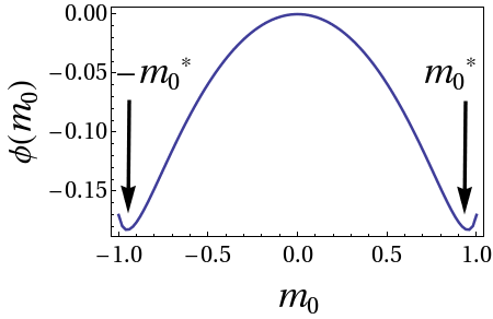
Figure 6: The large deviation function $\phi(m_{0})$ calculated using Eq. (3) and (6).

We now define a coarse-grained time variable $\tau=t/\Delta t$ such that the subsystem magnetization evolves with increasing $\tau$, however at any given $\tau$ each subsystem is effectively in the steady state corresponding to its magnetization. This separation of slow and fast processes is analogous to the adiabatic approximation in quantum mechanics ADIABATIC , and has also been applied in related models BEIJEREN ; COHEN .

Let us characterize the steady states corresponding to fixed sub-system magnetization $m_{0}$, $m_{u}$ and $m_{\ell}$. First consider the driven ring. In the limit $E\rightarrow\infty$ the dynamics within this ring is independent of the two other subsystems, and reduces to that of the Totally Asymmetric Simple Exclusion Process (TASEP). In its steady state all spin configurations with fixed magnetization $m_{0}$ are equally probable, leading to uniform magnetization and zero spin-spin correlation along the driven line. This steady state is reached in a time of $\mathcal{O}(L^{3/2})$ which, for $\gamma\ll L^{-3}$, is smaller than the typical time of exchange processes between the driven ring and its neighboring ones. Then, the driven ring provides an effective boundary magnetic field $Jm_{0}$ on the $u$ and $\ell$ subsystems. Thus the steady state of these two subsystems is the equilibrium state of the Ising model subjected to a boundary field. The boundary field results a magnetization profile, $m_{y}$, which for large $|y|$ approaches the bulk magnetization values $-m_{B}$ and $m_{B}$ for the $u$ and $\ell$ subsystems, respectively. The length scale of this approach is of the order of the spin-spin correlation length $\xi(T)$ of the $2D$ Ising model. Since this length is finite at all temperatures except at $T_{c}$ this demonstrates that the width of the interface remains finite for large $L$.

Let $P_{\tau}(m_{0})d\tau$ be the probability of the driven line magnetization to have value $m_{0}$ between coarse-grained time $\tau$ and $\tau+d\tau$, while $m_{u}$ and $m_{\ell}$ have already reached stationary values. The probability function evolves as spins are exchanged between the subsystems. At each exchange process between the driven ring and the bulk, $m_{0}$ changes by $\pm 2/L$. Let $p(m_{0})$ and $q(m_{0})$ be the increasing and decreasing rates of $m_{0}$, respectively. Then the dynamics of $m_{0}$ is that of a random walker with position dependent forward and backward jump rates $p(m_{0})$ and $q(m_{0})$, respectively, and with boundary condition $P_{\tau}(m_{0})=0$ for $|m_{0}|>1$.

The stationary distribution of this motion is an equilibrium distribution function,

$$P(m_{0})=P(0)\exp\left[-L\phi\left(m_{0}\right)\right].$$ (1)

The LDF $\phi(m_{0})$ is an even function of $m_{0}$ and it can be determined using the detailed balance condition $p(m_{0})P(m_{0})=q(m_{0}+2/L)P(m_{0}+2/L)$, which for $0<m_{0}\leq 1$ yields

$$P\left(m_{0}=\frac{2n}{L}\right)=P\left(0\right)\prod_{k=1}^{n}\frac{p\left[\frac{2}{L}(k-1)\right]}{q\left[\frac{2}{L}k\right]},$$ (2)

with $n=1,\dots,L/2$. In the large $L$ limit this yields the LDF for $m\geq 0$,

$$\phi(m_{0})=\frac{1}{2}\int_{0}^{m_{0}}dm\ln\left[\frac{p\left(m\right)}{q\left(m\right)}\right],$$ (3)

with $\phi(-m_{0})=\phi(m_{0})$.

The rates $p\left(m_{0}\right)$ and $q\left(m_{0}\right)$ are determined as follows: consider a spin exchange process between the driven ring and its two neighboring ones, in which the microscopic configuration changes from $\boldsymbol{\sigma}$ to $\boldsymbol{\sigma^{\prime}}$ and $m_{0}$ increases by $2/L$. The rate of this process is $\omega\left(\boldsymbol{\sigma}\rightarrow\boldsymbol{\sigma^{\prime}}\right)P\left(\boldsymbol{\sigma}|m_{0},-m_{B},m_{B}\right)$ where $\omega\left(\boldsymbol{\sigma}\rightarrow\boldsymbol{\sigma^{\prime}}\right)=\rm{min}\{1,\exp(-\beta\Delta H)\}$ is the Metropolis success rate in coarse grain time variable $\tau$ and $P\left(\boldsymbol{\sigma}|m_{0},-m_{B},m_{B}\right)$ is the steady state probability of configuration $\boldsymbol{\sigma}$ corresponding to subsystem magnetization $m_{0}$, $m_{u}=-m_{B}$ and $m_{\ell}=m_{B}$. Summing over all such exchanges one obtains

$$p\left(m_{0}\right)=\sum_{\boldsymbol{\sigma},\boldsymbol{\sigma^{\prime}}}\omega\left(\boldsymbol{\sigma}\rightarrow\boldsymbol{\sigma^{\prime}}\right)P\left(\boldsymbol{\sigma}|m_{0},-m_{B},m_{B}\right),$$ (4)

where the sum is over configurations $\boldsymbol{\sigma^{\prime}}$ whose $m_{0}$ is higher than that of $\boldsymbol{\sigma}$ by $2/L$. The magnetization decreasing rate $q(m_{0})$ is readily obtained by noting that due to the invariance of the dynamics to space-time inversion, $\sigma_{\mathbf{r}}\rightarrow-\sigma_{-\mathbf{r}}$, one has $q(m_{0})=p\left(-m_{0}\right)$.

In the slow exchange limit $\gamma\ll L^{-3}$, the probability $P\left(\boldsymbol{\sigma}|m_{0},-m_{B},m_{B}\right)$ can be expressed in terms of probability of the subsystem configurations as

$$P(\boldsymbol{\sigma}|m_{0},-m_{B},m_{B})\simeq P(\boldsymbol{\sigma}_{0}|m_{0})P\left(\boldsymbol{\sigma}_{u}|-m_{B},m_{0}\right)$$ (5)

$$P\left(\boldsymbol{\sigma}_{\ell}|m_{B},m_{0}\right),$$

where $\boldsymbol{\sigma}_{0}$, $\boldsymbol{\sigma}_{u}$ and $\boldsymbol{\sigma}_{\ell}$ are the microscopic spin configurations of the three subsystems corresponding to the configuration $\boldsymbol{\sigma}$. Here, $P(\boldsymbol{\sigma}_{0}|m_{0})$ is the steady state distribution of the driven line with fixed magnetization $m_{0}$, which is the same as the steady state of a TASEP, and $P\left(\boldsymbol{\sigma}_{u}|-m_{B},m_{0}\right)$ and $P\left(\boldsymbol{\sigma}_{\ell}|m_{B},m_{0}\right)$ are the equilibrium distribution of the other two subsystems.

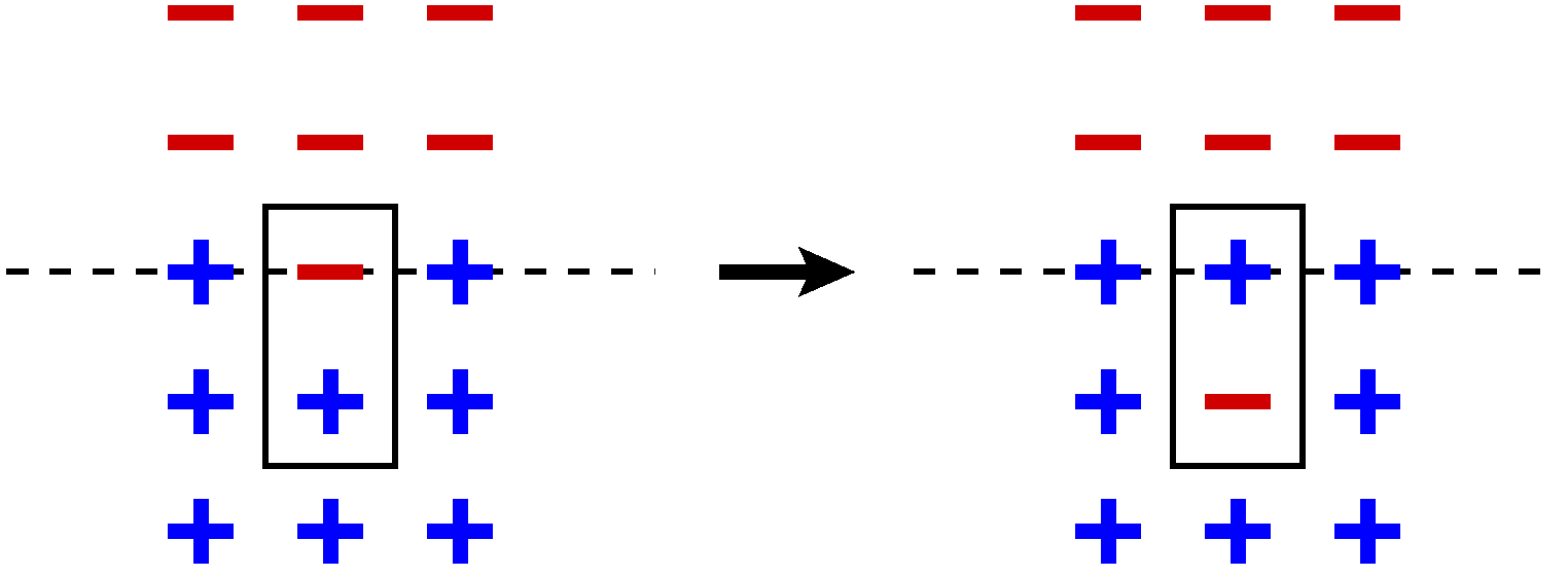
Figure 7: (color online) Spin exchange process which yields the leading order contribution to $p(m_{0})$. The driven ring is denoted by a dotted line, and the pair of spins exchanged are indicated.

In general, calculating all the terms in Eq. (4) is not straightforward. However, the calculation becomes feasible in the low $T$ limit where these rates may be expanded in powers of $\exp\left(-\beta J\right)$.

In order to keep track of the terms in this expansion it is convenient to generalize the model by considering an interaction strength between the driven ring and its neighboring ones as $J_{1}\leq J$. It is easy to see that the leading contribution to $p(m_{0})$ in Eq. (4) results from the exchange process shown in Fig. 7, where both subsystems $u$ and $\ell$ are in their respective ground state, $m_{\ell}=-m_{u}=1$. For this process $\omega\left(\boldsymbol{\sigma}\rightarrow\boldsymbol{\sigma^{\prime}}\right)=\exp(-2\beta(J+J_{1}))$ and $P\left(\boldsymbol{\sigma}|m_{0},-m_{B},m_{B}\right)=\left[\left(1+m_{0}\right)^{2}\left(1-m_{0}\right)/8\right]\left[1-\mathcal{O}\left(e^{-6\beta J}\right)\right]$. Higher order contributions can be determined similarly from other exchange events. Computing $p(m_{0})$ up to $\mathcal{O}(\exp(-6\beta J))$ yields, for $-1\leq m_{0}\leq 1$,

$$p\left(m_{0}\right)=\frac{1}{8}\left[\left(1+m_{0}\right)^{2}\left(1-m_{0}\right)e^{-2\beta J_{1}}\right]e^{-2\beta J}\\ +\frac{1}{8}\Bigl{[}\left(1+m_{0}\right)^{2}\left(1-m_{0}\right)\left(2e^{-2\beta J_{1}m_{0}}+e^{2\beta J_{1}m_{0}}\right)\\ +2\left(1+m_{0}\right)\left(1-m_{0}\right)^{2}\left(e^{-2\beta J_{1}}+e^{2\beta J_{1}m_{0}}\right)\\ +\left(1-m_{0}\right)^{3}e^{2J_{1}m_{0}}\Bigl{]}e^{-6\beta J}+\mathcal{O}\left(e^{-8\beta J}\right).$$ (6)

The LDF $\phi(m_{0})$ calculated using the rate in Eq. (6) is plotted in Fig. 6 for $\beta J_{1}=\beta J=3/4$ ($T\simeq 0.6T_{c}$). This function has two minima which correspond to the two thermodynamic phases with non-zero $m_{0}$. The average time $\tau_{s}$ for the magnetization to jump from one minimum to the other is proportional to the exponential of the barrier height between them. In terms of Monte Carlo steps this switching time $t_{s}\sim\gamma^{-1}\tau_{s}\sim\gamma^{-1}\exp(\epsilon L)$ where $\epsilon$ is the barrier height. For the parameters of Fig. 6 one has $\epsilon=0.18$ which is of the same order as that obtained numerically in Fig. 4. For a better comparison higher order terms in the low temperature expansion are required. The asymmetry in the fluctuations of the interface and the magnetization profile in Fig. 5 is a consequence of the non-zero values of $m_{0}$.

The analysis presented in this Letter demonstrates that a local drive can induce a phase transition which involves spontaneous symmetry breaking of an interface separating two coexisting phases. It would be interesting to consider other boundary conditions which would allow the interface to detach from the driven ring. This would correspond, for example, to studying the model with periodic boundary conditions in both the $x$ and $y$ directions. In this case the model exhibits two interfaces, and preliminary studies have shown that either one of them is attracted by the driven ring resulting in a macroscopic symmetry breaking, in addition to that of the interface ZVI . This will be addressed in a future publication.

- (1) D. Derks, D. G. A. L. Aarts, D. Bonn, H. N. W. Lekkerkerker, and A. Imhof, Phys. Rev. Lett. 97, 038301 (2006)
- (2) T. Sadhu, S. N. Majumdar, and D. Mukamel, Phys. Rev. E 84, 051136 (2011)
- (3) S. Katz, J. L. Lebowitz, and H. Spohn, Phys. Rev. B 28, 1655 (1983)
- (4) S. Katz, J. L. Lebowitz, and H. Spohn, J. Stat. Phys. 34, 497 (1984)
- (5) H. Spohn, J. Phys. A 16, 4275 (1983)
- (6) M. Q. Zhang, J. S. Wang, J. L. Lebowitz, and J. L. Vallés, J. Stat. Phys. 52, 1461 (1988)
- (7) P. L. Garrido, J. L. Lebowitz, C. Maes, and H. Spohn, Phys. Rev. A 42, 1954 (1990)
- (8) I. Pagonabarraga and J. M. Rubí, Phys. Rev. E 49, 267 (1994)
- (9) B. Schmittmann and R. Zia, in Statistical Mechanics of Driven Diffusive System, Phase Transitions and Critical Phenomena, Vol. 17, edited by C. Domb and J. Lebowitz (Academic Press, 1995)
- (10) T. H. R. Smith, O. Vasilyev, D. B. Abraham, A. Maciołek, and M. Schmidt, Phys. Rev. Lett. 101, 067203 (2008)
- (11) R. Dickman and R. R. Vidigal, J. Stat. Mech., P05003(2007)
- (12) K. Tsekouras and A. B. Kolomeisky, J. Phys. A 41, 465001 (2008)
- (13) A. Hucht, Phys. Rev. E 80, 061138 (2009)
- (14) H. J. Hilhorst, J. Stat. Mech., P04009(2011)
- (15) H. Touchette, Physics Reports 478, 1 (2009)
- (16) W. Kwak, D. P. Landau, and B. Schmittmann, Phys. Rev. E 69, 066134 (2004)
- (17) D. B. Abraham and P. Reed, Phys. Rev. Lett. 33, 377 (1974)
- (18) K.-t. Leung, K. K. Mon, J. L. Vallés, and R. K. P. Zia, Phys. Rev. Lett. 61, 1744 (1988)
- (19) K.-t. Leung, K. K. Mon, J. L. Vallés, and R. K. P. Zia, Phys. Rev. B 39, 9312 (1989)
- (20) A. Messiah, “Quantum mechanics,” (North Holland, Amsterdam, 1962) Chap. XVII, p. 750, 1st ed.
- (21) H. van Beijeren and L. S. Schulman, Phys. Rev. Lett. 53, 806 (1984)
- (22) O. Cohen and D. Mukamel, Phys. Rev. Lett. 108, 060602 (2012)
- (23) Z. Shapira, The effect of a driven line on a two-dimensional Ising system (M.Sc. Thesis, Weizmann Institute of Science, 2012)