The Luttinger liquid and integrable models

Abstract

Many fundamental one-dimensional lattice models such as the Heisenberg or the Hubbard model are integrable. For these microscopic models, parameters in the Luttinger liquid theory can often be fixed and parameter-free results at low energies for many physical quantities such as dynamical correlation functions obtained where exact results are still out of reach. Quantum integrable models thus provide an important testing ground for low-energy Luttinger liquid physics. They are, furthermore, also very interesting in their own right and show, for example, peculiar transport and thermalization properties. The consequences of the conservation laws leading to integrability for the structure of the low-energy effective theory have, however, not fully been explored yet. I will discuss the connection between integrability and Luttinger liquid theory here, using the anisotropic Heisenberg model as an example. In particular, I will review the methods which allow to fix free parameters in the Luttinger model with the help of the Bethe ansatz solution. As applications, parameter-free results for the susceptibility in the presence of non-magnetic impurities, for spin transport, and for the spin-lattice relaxation rate are discussed.

1 Introduction

The Tomonaga-Luttinger liquid [1, 2, 3, 4] is believed to describe the low-energy properties of gapless one-dimensional interacting electron systems irrespective of the precise nature of the microscopic Hamiltonian. This universality can be understood in a renormalization group sense as irrelevance of band curvature and additional interaction terms which might arise when deriving this low-energy effective theory from a microscopic model. Similar to the important role Onsager’s exact solution[5] of the two-dimensional Ising model has played in establishing and confirming general renormalization group theory, exactly solvable one-dimensional quantum models have been crucial for the development of Luttinger liquid theory.

Integrable models are, furthermore, also interesting in their own right and a number of almost ideal realizations are known today. One example are cuprate spin chains such as Sr₂CuO₃ whose magnetic properties are well described by the integrable one-dimensional Heisenberg model.[6, 7, 8, 9, 10, 11, 12, 13, 14] Furthermore, cold atomic gases represent quantum systems which are to a high degree isolated from the surroundings and whose Hamiltonians are easily tunable. This makes it possible to use them as quantum simulators to study almost perfect realizations of integrable systems such as the Lieb-Liniger model[15, 16] or the fermionic Hubbard model.[17]

In Sec.2 I will discuss quantum integrability with a particular emphasis on Bethe ansatz integrable models and outline possible effects on transport and the thermalization of closed quantum systems. In the rest of the paper, I will then concentrate on the anisotropic Heisenberg (or $XXZ$) model as one specific example for a Bethe ansatz integrable model. In Sec. 3 I describe how the Luttinger model, including leading irrelevant operators, can be obtained from this microscopic model by using bosonization techniques. In Sec. 4 I then briefly outline important aspects of the Bethe ansatz solution. In Sec. 5 it is shown that a comparison of the results of Sec. 3 and Sec. 4 allows to fix parameters in the Luttinger liquid theory for the $XXZ$ model. Applications of the parameter-free low-energy effective theory to calculate various properties of spin chains are considered in Sec. 6. This includes the calculation of susceptibilities in the presence of non-magnetic impurities, and results for spin transport and NMR relaxation rates. The final section is devoted to a brief summary and some conclusions.

2 Quantum integrability

A classical system with Hamilton function $\mathcal{H}$ and phase space dimension $2N$ is integrable if it has $N$ constants of motion $\mathcal{Q}_{n}$ with

$$\{\mathcal{H},\mathcal{Q}_{n}\}=0\quad\mbox{and}\quad\{\mathcal{Q}_{i},\mathcal{Q}_{j}\}=0\quad\mbox{if}\quad i\neq j\,.$$ (1)

Here $\{.,.\}$ denotes the Poisson bracket. Quantum integrability, on the other hand, is much harder to define precisely, see, for example, Ref. 18. In this regard it is important to note that every quantum system in the thermodynamic limit, irrespective of integrability, has infinitely many conservation laws

$$[H,|E_{n}\rangle\langle E_{n}|]=0$$ (2)

where $H$ is the Hamiltonian with eigenstates $|E_{n}\rangle$ and $[.,.]$ denotes the commutator. Apart from these non-local conservation laws a quantum system can have local conservation laws given by

$$\mathcal{Q}_{n}=\sum_{j}q_{n,j}\quad\mbox{or}\quad\mathcal{Q}_{n}=\int dx\,q_{n}(x)$$ (3)

where $q_{n,j}$ is a density operator acting on $n$ neighboring sites in the case of a lattice model while for a continuum model $q_{n}(x)$ is a fully local density operator. A generic example for a local conservation law is the Hamiltonian itself for models with short range interactions. In Bethe ansatz integrable models a whole set of such local conservation laws does exist which can be obtained from the transfer matrix of the corresponding two-dimensional classical model by taking successive derivatives of the transfer matrix $\tau$ with respect to the spectral parameter $\lambda$

$$\mathcal{Q}_{n}\propto\frac{\partial^{n}}{\partial\lambda^{n}}\ln\tau(\lambda)\bigg{|}_{\lambda=\xi}\,.$$ (4)

Here $\xi$ is the spectral parameter at which the transfer matrix is evaluated. These conserved quantities are directly related to the existence of so-called $R$-matrices which fulfill the Yang-Baxter equations and from which the transfer matrices $\tau(\lambda)$ can be constructed.[19]

For a low-energy effective theory describing such an integrable model, we have to demand—at least in principle—that the low-energy Hamiltonian $H_{\rm eff}$ also fulfills

$$[H_{\rm eff},\mathcal{Q}_{n}]=0.$$ (5)

This corresponds to a fine-tuning of parameters in the Luttinger model. In particular, it might mean that certain terms which are not forbidden by general symmetry considerations have to vanish. Such a program has not fully been explored yet; in Sec. 5.2 we will see, as an example, that the conserved quantity $\mathcal{Q}_{3}$ for the $XXZ$ model does indeed prevent certain terms from occuring in the low-energy theory.

2.1 Consequences for transport

Local conservation laws can have a dramatic effect on the transport properties.[20] This can be easily understood as follows. We can always define a local current density $j_{l}$ by making use of the continuity equation

$$\frac{\partial}{\partial t}\rho_{l}+j_{l}-j_{l-1}=0$$ (6)

where $\rho_{l}$ is the density at site $l$. The current itself is then given by $\mathcal{J}=\sum_{l}j_{l}$. This current could be, for example, an electric, spin or thermal current. Conserved quantities $Q_{n}$ can now prevent a current from decaying completely leading to ballistic transport and a finite Drude weight

$$D(T)\equiv\lim_{t\to\infty}\lim_{L\to\infty}\frac{1}{2LT}\langle\mathcal{J}(t)\mathcal{J}(0)\rangle\geq\lim_{L\to\infty}\frac{1}{2LT}\sum_{n}\frac{\langle\mathcal{J}Q_{n}\rangle^{2}}{\langle Q_{n}^{2}\rangle}\,.$$ (7)

Here $Q_{n}$ can denote a local or non-local conserved quantity, $L$ is the length of the system, and $T$ the temperature. The second relation in Eq. (7) is the Mazur inequality[21] which becomes an equality if all conservation laws, local and non-local, are included.[22, 23] In order to obtain a possible non-zero Drude weight at finite temperatures within a Luttinger model description, the relevant conservation laws have to be taken into account explicitly. One way to achieve this is discussed in Sec. 6.2. Importantly, one expects that only local or pseudo-local conservation laws $\mathcal{Q}_{n}$ with $\langle\mathcal{J}\mathcal{Q}_{n}\rangle\neq 0$ can give rise to a finite bound in Eq. (7) so that $D(T>0)\neq 0$ is characteristic for an integrable model.

2.2 Consequences for thermalization in closed systems

Additional local conservation laws can also have a profound impact on a possible thermalization of a closed quantum system. Imagine that we prepare an initial state $|\Psi(0)\rangle$ and follow the unitary time evolution of this state under an integrable Hamiltonian. One says that a closed quantum system in the thermodynamic limit has thermalized if for any local observable $\mathcal{O}$ the limit

$$\mathcal{O}_{\infty}=\lim_{t\to\infty}\langle\Psi(t)|\mathcal{O}|\Psi(t)\rangle$$ (8)

is well-defined and time independent and can also be expressed as an ensemble average

$$\mathcal{O}_{\infty}\equiv\mbox{Tr}(\mathcal{O}\rho)$$ (9)

with an appropriately chosen density matrix $\rho$. Note that even for a generic closed quantum system temperature $T$ is not defined by an external bath but rather by the energy of the initial state

$$\langle\Psi(0)|H|\Psi(0)\rangle=\underbrace{\mbox{Tr}(H\mbox{e}^{-H/T})/Z}_{\mbox{Tr}(\rho_{c}H)}$$ (10)

with $T$ acting as a Lagrange multiplier and $Z$ being the partition function. For an integrable model we have to demand that the relation (10) also holds if we replace $H\to\mathcal{Q}_{n}$ and the canonical density matrix $\rho_{c}$ by the density matrix[24]

$$\rho=\frac{1}{Z}\exp\bigg{(}-\sum_{j}\lambda_{j}\mathcal{Q}_{j}\bigg{)}$$ (11)

which now contains a Lagrange multiplier $\lambda_{j}$ for each of the locally conserved quantities. The existence of additional local conservation laws therefore severely restricts a possible thermalization of the system leading to additional constraints which are incorporated by the Lagrange multipliers in Eq. (11). Experimental indications for such constraints have been seen in realizations of the Lieb-Liniger model in ultracold gases.[16]

3 Low-energy description of the $XXZ$ model

In the following sections, we want to concentrate on one of the simplest integrable lattice models, the $XXZ$ model

$$H=J\sum_{j=1}^{N(N-1)}\left[-\frac{1}{2}\left(c_{j}^{\dagger}c_{j+1}^{\phantom{\dagger}}+h.c.\right)-h\left(c_{j}^{\dagger}c_{j}^{\phantom{\dagger}}-\frac{1}{2}\right)+\Delta\left(n_{j}-\frac{1}{2}\right)\left(n_{j+1}-\frac{1}{2}\right)\right].$$ (12)

Here $c$ ($c^{\dagger}$) annihilates (creates) a spinless fermion, $J$ gives the energy scale, $\Delta$ characterizes the nearest neighbor density-density interaction with the density operator $n_{j}=c^{\dagger}_{j}c_{j}$. $N$ is the number of sites and the boundary conditions might be either periodic (sum runs up to $N$ with $c^{(\dagger)}_{N+1}\equiv c^{(\dagger)}_{1}$) or open (sum runs only up to $N-1$). $h$ acts as a chemical potential. With the help of the Jordan-Wigner transformation

$$S_{j}^{z}\rightarrow n_{j}-\frac{1}{2},\quad S_{j}^{+}\rightarrow\left(-1\right)^{j}\,c_{j}^{\dagger}e^{i\pi\phi_{j}},\quad S_{j}^{-}\rightarrow\left(-1\right)^{j}\,c_{j}^{\phantom{\dagger}}e^{-i\pi\phi_{j}},$$ (13)

where $\phi_{j}=\sum_{l=1}^{j-1}n_{l}$ we can also express this model in terms of spin-$1/2$ operators

$$H=J\sum_{j=1}^{N(N-1)}[S^{x}_{j}S^{x}_{j+1}+S^{y}_{j}S^{y}_{j+1}+\Delta S^{z}_{j}S^{z}_{j+1}-hS^{z}_{j}]\,.$$ (14)

For both kinds of boundary conditions the $XXZ$ model is integrable by Bethe ansatz.[25, 17, 26, 27, 28] The Luttinger liquid approach is applicable in the critical regime which is given by $-1<\Delta\leq 1$ for $h=0$. In general, the range of anisotropies for which the model is critical depends on the applied magnetic field $h$. In the free fermion case, the model (12) is easily solved by Fourier transform leading to

$$H_{0}=\sum_{p}\epsilon_{p}c_{p}^{\dagger}c_{p}\quad\mbox{with}\quad\epsilon_{p}=-J(\cos p+h)\,.$$ (15)

where we have set the lattice constant $a=1$. The allowed momenta are given by $p=2\pi n/N$ with $n=0,\cdots,N-1$ for periodic boundary conditions (PBCs) or $p=\pi n/(N+1)$, $n=1,\cdots,N$ for open boundary conditions (OBCs). In Sec. 4 we will briefly discuss the Bethe ansatz solution of this model for OBCs.

Let us first revisit the derivation of an effective low-energy description, the Luttinger theory, by bosonization following Refs. 29, 4, 30. First, we replace the fermionic operators in the continuum limit by two fields $\psi_{R,L}$ defined near the two Fermi points $\pm k_{F}=\pm\arccos(-h)$:

$$c_{j}\rightarrow\psi\left(x\right)=e^{ik_{F}x}\psi_{R}\left(x\right)+e^{-ik_{F}x}\psi_{L}\left(x\right).$$ (16)

In a second step, we use standard Abelian bosonization to write the fermion fields as

$$\psi_{R,L}\left(x\right)\sim\frac{1}{\sqrt{2\pi\alpha}}\,e^{-i\sqrt{2\pi}\phi_{R,L}\left(x\right)},$$ (17)

where $\alpha\sim k_{F}^{-1}$ is a short distance cutoff. Instead of working with the left and right components $\phi_{R,L}$ we can define a bosonic field $\tilde{\phi}$ and its dual field $\tilde{\theta}$ by

$$\tilde{\phi}=\frac{\phi_{L}-\phi_{R}}{\sqrt{2}},\qquad\tilde{\theta}=\frac{\phi_{L}+\phi_{R}}{\sqrt{2}},$$ (18)

which satisfy the standard bosonic commutation rule $[\tilde{\phi}\left(x\right),\partial_{x^{\prime}}\tilde{\theta}\left(x^{\prime}\right)]=i\delta\left(x-x^{\prime}\right)$.

If we bosonize the kinetic energy term of Eq. (12) keeping only the lowest order we obtain

$$H_{0}^{kin}=iv_{F}\int_{0}^{L}\!\!dx\,\left(:\psi_{R}^{\dagger}\partial_{x}\psi_{R}^{\phantom{\dagger}}:\,-\,:\psi_{L}^{\dagger}\partial_{x}\psi_{L}^{\phantom{\dagger}}:\right)=\frac{v_{F}}{2}\int_{0}^{L}\!\!dx\,\left[\left(\partial_{x}\phi_{R}\right)^{2}+\left(\partial_{x}\phi_{L}\right)^{2}\right]$$ (19)

where $:\,:$ denotes normal ordering and $v_{F}=J\sin k_{F}$ is the Fermi velocity. This approximation corresponds to a linearization of the dispersion $\epsilon_{p}$ at the Fermi points $\pm k_{F}$. In this case the bosonic model is quadratic in $\partial_{x}\phi_{R,L}$. Corrections to the kinetic energy appear due to band curvature. Including these curvature terms, we can write the expansion of the dispersion $\epsilon_{p}$ near the two Fermi points as

$$\epsilon_{k}^{R,L}\approx\pm v_{F}k+\frac{k^{2}}{2M}\mp\frac{\gamma k^{3}}{6}+\dots,$$ (20)

where $k\equiv p\mp k_{F}$ for the right or left movers, respectively, $M=\left(J\cos k_{F}\right)^{-1}$ is the effective mass and $\gamma=J\sin k_{F}$. Note that the inverse mass $M^{-1}$ vanishes in the particle-hole symmetric case $h=0$. In this case, the curvature correction is cubic in momentum. Bosonization of the $k^{2}$-term leads to a correction cubic in $\partial_{x}\phi_{R,L}$, whereas the term cubic im momentum gives a quartic correction in terms of the bosonic fields. Cubic and quartic terms in the bosonic operators will also arise from the interaction term in Eq. (12). The scaling dimension of these terms is $3$ respectively $4$ so that they are formally irrelevant. The interaction will, however, also produce additional marginal terms, quadratic in the bosonic fields, which together with (19) lead to the exactly solvable Luttinger model

$$H_{LL}=\frac{v_{F}}{2}\int dx\left\{\left(1+\frac{g_{4}}{2\pi v_{F}}\right)\left[\left(\partial_{x}\phi_{R}\right)^{2}+\left(\partial_{x}\phi_{L}\right)^{2}\right]\right.\left.-\frac{g_{2}}{\pi v_{F}}\,\partial_{x}\phi_{L}\partial_{x}\phi_{R}\right\}.$$ (21)

Here $g_{2}=g_{4}=2J\Delta[1-\cos(2k_{F})]=4J\Delta\sin^{2}k_{F}$ are interaction parameters. The Hamiltonian (21) can be rewritten in the form

$$H_{LL}=\frac{1}{2}\int dx\,\left[vK\left(\partial_{x}\tilde{\theta}\right)^{2}+\frac{v}{K}\left(\partial_{x}\tilde{\phi}\right)^{2}\right],$$ (22)

where $v$ (the renormalized velocity) and $K$ (the Luttinger parameter) are given by

$$v = v_{F}\sqrt{\left(1+\frac{g_{4}}{2\pi v_{F}}\right)^{2}-\left(\frac{g_{2}}{2\pi v_{F}}\right)^{2}}\approx v_{F}\left(1+\frac{2\Delta}{\pi}\sin k_{F}\right),$$ (23)

$$K = \sqrt{\frac{1+\frac{g_{4}}{2\pi v_{F}}-\frac{g_{2}}{2\pi v_{F}}}{1+\frac{g_{4}}{2\pi v_{F}}+\frac{g_{2}}{2\pi v_{F}}}}\approx 1-\frac{2\Delta}{\pi}\sin k_{F}.$$ (24)

Expressions (23) and (24) are approximations valid in the limit $|\Delta|\ll 1$. In Sec. 5 we will review how these parameters in the Luttinger liquid Hamiltonian can be fixed exactly for arbitrary interaction strengths $-1<\Delta\leq 1$ using the Bethe ansatz solution.

The Luttinger parameter in the Hamiltonian (22) can be absorbed by performing a canonical transformation that rescales the fields in the form $\tilde{\phi}\rightarrow\sqrt{K}\phi$ and $\tilde{\theta}\rightarrow\theta/\sqrt{K}$ leading to

$$H_{LL}=\frac{v}{2}\int dx\,\left[\left(\partial_{x}\theta\right)^{2}+\left(\partial_{x}\phi\right)^{2}\right].$$ (25)

We can also define the right and left components of these rescaled bosonic fields by

$$\varphi_{R,L}=\frac{\theta\mp\phi}{\sqrt{2}}.$$ (26)

These are related to $\phi_{R,L}$ by a Bogoliubov transformation.

3.1 Irrelevant operators in the finite field case

The leading irrelevant operators stem from the $k^{2}$-term in Eq. (20) and give rise to dimension three operators $\sim(\partial_{x}\phi_{R,L})^{3}$. Similar terms will also arise by bosonizing the interaction term. Instead of deriving these terms from the microscopic Hamiltonian, we can introduce them phenomenologically by considering the symmetries of the problem. In particular, the low-energy effective theory has to be symmetric under the parity transformation $\phi_{L}\to\phi_{R}$, $\phi_{R}\to\phi_{L}$, and $x\to-x$. We therefore can parametrize these terms as[30]

$$\delta H=\frac{\sqrt{2\pi}}{6}\int dx\,\left\{\eta_{-}\left[\left(\partial_{x}\varphi_{L}\right)^{3}-\left(\partial_{x}\varphi_{R}\right)^{3}\right]\right.\left.+\eta_{+}\left[\left(\partial_{x}\varphi_{L}\right)^{2}\partial_{x}\varphi_{R}-\left(\partial_{x}\varphi_{R}\right)^{2}\partial_{x}\varphi_{L}\right]\right\}.$$ (27)

We will see in Sec. 5 that we can relate the amplitudes $\eta_{\pm}$ to quantities which are known from the exact solution. The derivation of these terms starting from the microscopic Hamiltonian, on the other hand, would only allow us to obtain the coupling constants to first order in $\Delta$ with[30]

$$\eta_{-}\approx\frac{1}{M}\left(1+\frac{2\Delta}{\pi}\sin k_{F}\right),\quad\eta_{+}\approx-\frac{3\Delta}{\pi M}\sin k_{F}.$$ (28)

From this expansion we see that (a) both terms vanish in the limit $h\to 0$ where $M^{-1}\to 0$, and (b) that the term mixing right and left movers parametrized by $\eta_{+}$ is only present in the interacting case, $\Delta\neq 0$.

3.2 Irrelevant operators for zero field

In the particle-hole symmetric case, $h=0$, the first correction to the linear dispersion relation is cubic in momentum, see Eq. (20). Instead of bosonizing this term starting from the microscopic Hamiltonian (12) we again introduce the corresponding terms in the bosonic model based on symmetry arguments. The dimension four operators allowed by symmetry can be parametrized as

$$\delta\mathcal{H} = \frac{\pi\zeta_{-}}{12}\left[:\left(\partial_{x}\varphi_{R}\right)^{2}:\,:\left(\partial_{x}\varphi_{R}\right)^{2}:+:\left(\partial_{x}\varphi_{L}\right)^{2}:\,:\left(\partial_{x}\varphi_{L}\right)^{2}:\right]+\frac{\pi\zeta_{+}}{2}\,\left[:\left(\partial_{x}\varphi_{R}\right)^{2}:\right.$$ (29)

$$\left.:\left(\partial_{x}\varphi_{L}\right)^{2}:\right]+\pi\zeta_{3}\left[:(\partial_{x}\varphi_{R})^{3}:\,:\partial_{x}\varphi_{L}:+:(\partial_{x}\varphi_{L})^{3}:\,:\partial_{x}\varphi_{R}:\right]\,.$$

The explicit bosonization of the corresponding band curvature and interaction terms yields the coupling constants again only to lowest lowest order

$$\zeta_{-}\approx-J\left(1+\frac{\Delta}{\pi}\right),\qquad\zeta_{+}\approx-\frac{\Delta J}{\pi},\qquad\zeta_{3}=0.$$ (30)

In addition, the Umklapp scattering term $\delta\mathcal{H}_{U}\sim\mbox{e}^{4ik_{F}x}\Psi_{R}^{\dagger}(x)\Psi_{L}(x)\Psi_{R}^{\dagger}(x+1)\Psi_{L}(x+1)+h.c.$ is commensurate in this case, $4k_{F}=2\pi$, and therefore has to be kept in the low-energy effective theory. Bosonizing this term leads to

$$\delta\mathcal{H}_{U}=\lambda\cos(4\sqrt{\pi K}\phi)\,,$$ (31)

and to lowest order in $\Delta$ we have $\lambda=J\Delta/(2\pi^{2})$. For OBC, there is also an irrelevant boundary operator allowed

$$\delta\mathcal{H}_{B}\sim(\delta(x)+\delta(L))(\partial_{x}\phi)^{2}\,.$$ (32)

Finally, we want to consider the Luttinger model (25) with an additional small magnetic field $\delta h$ added, ignoring the irrelevant terms

$$H=\frac{v}{2}\int_{0}^{L}\left[(\partial_{x}\phi)^{2}+(\partial_{x}\theta)^{2}-\frac{2}{v}\sqrt{\frac{K}{\pi}}\delta h\partial_{x}\phi\right]\,.$$ (33)

By performing a shift in the boson field

$$\phi\to\phi+\sqrt{\frac{K}{\pi}}\frac{x}{v}\delta h$$ (34)

we return to the quadratic Hamiltonian (25) with an additional constant shift $-LK(\delta h)^{2}/(2\pi v)$. The bulk susceptibility per site is therefore given by

$$\chi_{\rm bulk}=K/\pi v\,.$$ (35)

This result does not only hold for $h=0$ but also for any finite field $h_{0}$ at which we want to calculate $\chi$ with $K=K(\Delta,h_{0})$ and $v=v(\Delta,h_{0})$.

4 The Bethe ansatz solution

To exactly solve the interacting system for PBC or OBC, one can use the coordinate Bethe ansatz.[25, 17, 28, 27, 26] Here we want to review very briefly some of the essential results needed to fix the parameters in the Luttinger model and refer the reader to Refs. 28, 31, 32, 33 for a more detailed discussion. The coordinate Bethe ansatz starts from the fully polarized state (’the vacuum’) and one derives coupled eigenvalue equations $H|M\rangle=E|M\rangle$ for states $|M\rangle$ with $M$ spins flipped. The eigenenergies can then be written as

$$E=J\sum_{j=1}^{M}\cos k_{j}+J\Delta\left(\frac{N-1}{4}-M\right)\,.$$ (36)

The structure is similar to the non-interacting case, however, the momenta $k_{j}$ are shifted from their positions for $\Delta=0$. They can be determined from a set of coupled nonlinear equations. In the thermodynamic limit, a single integral equation for the density of roots $\rho(x)$ is obtained which parametrizes the allowed momenta

$$\vartheta(x,\gamma)+\frac{1}{2N}\left[\vartheta(x,\gamma)+\vartheta(x,\pi-\gamma)+\vartheta(x,2\gamma)\right]=\rho(x)+\int_{-B}^{B}\vartheta(x-y,2\gamma)\rho(y)\,dy,$$ (37)

where

$$\vartheta(x,\gamma)=\frac{1}{\pi}\frac{\sin\gamma}{\cosh 2x-\cos\gamma}$$ (38)

and we have set $\Delta=\cos\gamma$. Eq. (37) is the integral equation for the $XXZ$ chain with OBC in the thermodynamic limit, including the boundary correction $\sim\mathcal{O}(1/N)$. Omitting the $1/N$ correction this is the standard integral equation for PBC.[28] The integral equation contains an unknown parameter $B$ and an unknown function $\rho(x)$. It can be solved analytically by Fourier transform for $B=\infty$ and one finds (ignoring the $1/N$ correction)

$$\rho(x)=\frac{1}{2\gamma\cosh\pi x/\gamma}\,.$$ (39)

The magnetization per site $m$ and the ground state energy per site $e$ for general $B$ are given by

$$m = 1/2-\int_{-B}^{B}\rho(x)dx+1/(2N)$$

$$e = -hs^{z}-\frac{J\sin\gamma}{2}\int_{-B}^{B}\vartheta(x,\gamma)\rho(x)dx+\frac{J}{4}\left(\cos\gamma+\frac{2-\cos\gamma}{N}\right).$$ (40)

Inserting (39) into Eq. (40) one finds that $B=\infty$ corresponds to $m=0$, i.e., to the case of zero magnetic field $h=0$. In general, $B=B(h)$ and the dependence on magnetic field has to be determined numerically. This can be achieved by using the stationarity condition

$$\frac{\partial}{\partial B}[e(h)-e(h=0)]=0.$$ (41)

5 Fixing parameters of the Luttinger model using integrability

One of the main motivations to apply Luttinger liquid theory to integrable models is that parameters in the Luttinger liquid theory such as velocities, Luttinger parameters, coupling constants of irrelevant operators and prefactors of correlation functions which usually are non-universal and therefore unknown, can often be determined in the case of an integrable model.[31, 34, 35, 36, 37] This makes it possible to obtain parameter-free results at low energies. The general idea is to calculate static observables at zero or finite temperatures exactly using the Bethe ansatz and to compare with results obtained within Luttinger theory. In the following we briefly review this method to obtain the velocity and Luttinger liquid parameter, Sec. 5.1, and the coupling constants for band curvature and Umklapp terms for the $XXZ$ model, Sec. 5.2.

5.1 Velocity and Luttinger liquid parameter

To obtain the velocity of elementary excitations, we have to consider the change in energy when replacing the ground state distribution of roots by a distribution which contains an excitation near the Fermi points. In the case of finite magnetic field, the obtained Bethe ansatz equations can only be solved numerically. Here we want to restrict ourselves to the zero field case. Replacing the ground state distribution (39) in the expression for the energy (40) by the distribution containing an excitation gives the energy in terms of the momentum change.[28] This allows to read off the spin velocity

$$v=\frac{\partial E}{\partial k}\bigg{|}_{k=k_{F}}=\frac{J\pi}{2}\frac{\sin\gamma}{\gamma}=\frac{J\pi}{2}\frac{\sqrt{1-\Delta^{2}}}{\arccos\Delta}\,.$$ (42)

The spin velocity therefore increases from $v_{F}=J$ (remember that we have set $a=1$) at the free fermion point to $v=J\pi/2$ at the isotropic antiferromagnetic Heisenberg point. Conversely, the velocity vanishes, as expected, for $\Delta\to-1$ corresponding to the isotropic ferromagnet.

To determine the Luttinger parameter $K$ it is easiest to calculate the bulk susceptibility $\chi_{\rm bulk}(h)=\partial m/\partial h$ using Eq. (40). To do so, $B(h)$ is required. For finite magnetic fields this again requires a numerical solution. For infinitesimal fields, on the other hand, $B(h)$ can be determined analytically [28, 32, 33] and

$$\chi_{\mbox{\footnotesize bulk}}=\frac{1}{J}\frac{\gamma}{(\pi-\gamma)\pi\sin\gamma}=\frac{1}{2v(\pi-\gamma)}$$ (43)

is obtained. Comparing with Eq. (35) we find

$$K=\frac{\pi}{2(\pi-\gamma)}=\frac{\pi}{2(\pi-\arccos\Delta)}\,.$$ (44)

Therefore $K=1$ for the free fermion model and $K=1/2$ at the isotropic antiferromagnetic Heisenberg point. Eq. (42) and Eq. (44) agree to first order with the expressions (24). The velocity and Luttinger parameter, both for zero and finite fields, as obtained from the Bethe ansatz solution, are shown in Fig. 1.

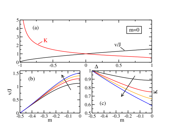
Figure 1: (a) Velocity $v/J$ and Luttinger parameter $K$ for magnetization $m=0$ as a function of $\Delta$. Velocity (b) and Luttinger parameter (c) as a function of magnetization $m$ for $\Delta=0.2,0.5,0.7,0.9$ (in arrow direction).

5.2 Coupling constants of irrelevant operators

Next, we want to review how the coupling constants $\zeta_{\pm,3}$, Eq. (29), and $\lambda$, Eq. (31), can be fixed in the zero field case, and the coupling constants $\eta_{\pm}$, Eq. (27), for finite field. The zero field case has been first considered by Lukyanov[31] and analytical formulas for the coupling constants have been obtained. The finite field case has been treated in Refs. 38, 30 leading to formulas which require a numerical solution of the Bethe ansatz equations.

5.2.1 The zero field case

The simplest way to determine the Umklapp scattering amplitude $\lambda$ is to consider an open chain with a small magnetic field added.[33] In the low-energy description this means that we have to consider (33) with the Umklapp term (31) added. We can then again perform the shift (34). This brings us back to the standard Luttinger liquid Hamiltonian (25) and the magnetic field now appears in the Umklapp term (31). In first order perturbation theory in Umklapp scattering we then find the following boundary correction to the ground state energy[39]

$$E_{U}^{(1)}=\lambda\int_{0}^{\infty}dx\left\langle\cos\left(4\sqrt{\pi K}\phi+\frac{4Khx}{v}\right)\right\rangle_{0}\,.$$ (45)

Here $\langle\cdots\rangle_{0}$ denotes the correlation function calculated for the free boson model. For PBC this correlation function would vanish, however, for OBC we obtain

$$E_{U}^{(1)}=\lambda\int_{0}^{\infty}dx\frac{\cos\left(\frac{4Khx}{v}\right)}{(2x)^{4K}}\;.$$ (46)

Note that this is a $1/N$ correction to the ground state energy per site $e=E/N$. By partial integration we can split of the convergent part and find

$$E_{U}^{(1,conv)}=-\lambda(2K)^{4K}\Gamma(-4K)\sin(2K\pi)\left(\frac{h}{v}\right)^{4K-1}\;.$$ (47)

At the same time, we can apply the Bethe ansatz to analytically calculate the so-called boundary susceptibility $\chi_{B}$ given by $\chi=\chi_{\rm bulk}+\chi_{B}/N+\mathcal{O}(N^{2})$ to leading orders in $h$.[33, 32] The amplitude $\lambda$ of the Umklapp term can now be found by comparing the exact result for $\chi_{B}$ with Eq. (47). This leads to

$$\lambda=\frac{2K\Gamma(2K)\sin\pi/2K}{\pi\Gamma(2-2K)}\left[\frac{\Gamma\left(1+\frac{1}{4K-2}\right)}{2\sqrt{\pi}\Gamma\left(1+\frac{K}{2K-1}\right)}\right]^{4K-2}\,.$$ (48)

In Ref. 31 this result has been obtained first by calculating the bulk correction to the ground state energy. Note, however, that this requires second order perturbation theory in the Umklapp scattering. Particular care has to be taken when considering the isotropic antiferromagnet, $\Delta=1$. In this case, Umklapp scattering becomes marginally irrelevant and $\lambda$ has to be replaced by a running coupling constant which depends on the length scale the system is considered at. In general, both the length of the system and temperature will be of importance and the running coupling constant $g(L,v/T)$ can be introduced by the replacements $K\to(1+g)/2$ and $\lambda\to-g/4$. An explicit solution of the renormalization group equations for $g$ is only possible if one of those two length scales dominates. In the thermodynamic limit, for example, this scale will be set by temperature alone and one finds[31]

$$1/g+\ln(g)/2=\ln(T_{0}/T)$$ (49)

with $T_{0}=\sqrt{\pi/2}\mbox{e}^{1/4+\tilde{\gamma}}$ where $\tilde{\gamma}$ is the Euler constant. The scale $T_{0}$ has again been fixed by comparing with the Bethe ansatz result for the bulk susceptibility $\chi_{\rm bulk}$ in the isotropic case.

Here integrability has been used to fix a coupling constant. The conservation laws underlying integrability discussed in Sec. 2 can, however, have an even more profound effect.[13, 14] For the $XXZ$ model the first of the non-trivial conserved quantities is the energy current $J^{E}=\mathcal{Q}_{3}$ given by

$$J^{E} = J^{2}\sum_{j}\left[S_{j-1}^{y}S_{j}^{z}S_{j+1}^{x}-S_{j-1}^{x}S_{j}^{z}S_{j+1}^{y}+\Delta(S_{j-1}^{x}S_{j}^{y}S_{j+1}^{z}-S_{j-1}^{z}S_{j}^{y}S_{j+1}^{x})\right.$$ (50)

$$\left.+\Delta(S_{j-1}^{z}S_{j}^{x}S_{j+1}^{y}-S_{j-1}^{y}S_{j}^{x}S_{j+1}^{z})\right].$$

The latter is defined by the continuity equation of the energy density at zero field

$$j^{E}_{j+1}-j^{E}_{j}=-\partial_{t}\mathcal{H}_{j}=i[\mathcal{H}_{j},H],$$ (51)

where $H=\sum_{j}\mathcal{H}_{j}$ is the Hamiltonian (14) with $h=0$, PBC, and $J^{E}=\sum_{j}j^{E}_{j}$. The energy current operator for the Luttinger model can be obtained from (51) by taking the continuum limit. This leads to

$$J^{E}_{0}=\int dx\,j^{E}_{0}(x)=\frac{v^{2}}{2}\int dx\left[\left(\partial_{x}\varphi_{R}\right)^{2}-\left(\partial_{x}\varphi_{L}\right)^{2}\right]=-v^{2}\int dx\,\partial_{x}\phi\partial_{x}\theta.$$ (52)

This operator is conserved, i.e., $[J_{0}^{E},H_{LL}]=0$. The irrelevant operators (29) lead to a correction of the energy current which can again be calculated using the continuity equation (51). To first order one finds

$$\delta J^{E}=\pi v\int dx\left\{\frac{\zeta_{-}}{3}\left[\left(\partial_{x}\varphi_{R}\right)^{4}-\left(\partial_{x}\varphi_{L}\right)^{4}\right]\right.\left.+2\zeta_{3}\left[\left(\partial_{x}\varphi_{R}\right)^{3}\partial_{x}\varphi_{L}-\left(\partial_{x}\varphi_{L}\right)^{3}\partial_{x}\varphi_{R}\right]\right\}.$$ (53)

For $J^{E}=J_{0}^{E}+\delta J^{E}$ to be conserved as required by integrability, we have to require that $[J^{E},H]=[J_{0}^{E}+\delta J^{E},H_{LL}+\delta H]=0$ up to the considered order. Since $[J^{0}_{E},H]=[J_{0}^{E},H_{LL}+\delta H]=0$ this implies that $[\delta J^{E},H_{LL}]=0$. The $\zeta_{-}$-term in Eq. (53) does not mix right and left movers and therefore obviously commutes with $H_{LL}$. The $\zeta_{3}$-term, on the other hand, does mix the two modes and therefore does not commute with $H_{LL}$. Integrability therefore implies that $\zeta_{3}=0$. We see that apart from determining the precise values of coupling constants in the low-energy effective theory, there is a more fundamental consequence: Integrability corresponds to a fine tuning of the coupling constants such that the local conservation laws are fulfilled. In particular, terms which are in general allowed by symmetry might be absent.

We are left with only two amplitudes, $\zeta_{\pm}$, for the dimension four operators. Let us briefly review how they can be fixed as well. Using Eq. (26) we can express both terms by the boson field $\phi$ and the dual field $\theta$. Now performing again the shift (34) for a small applied magnetic field $\delta h$ we find a first order correction to the ground state energy per site

$$e^{(1)}_{\zeta_{\pm}}=(\zeta_{-}+3\zeta_{+})\frac{K^{2}(\delta h)^{4}}{24\pi v^{4}}\,.$$ (54)

The $(\delta h)^{4}$-term in the ground state energy can also be calculated analytically by Bethe ansatz.[31, 32, 33] One finds that the result consists of two distinct, additive, contributions. One of those vanishes at the free fermion point and is therefore associated with the $\zeta_{+}$-term in the low-energy effective theory which mixes right and left movers. The other term then determines $\zeta_{-}$ leading to[31]

$$\zeta_{-}=-\frac{v}{4\pi K}\frac{\Gamma\left(\frac{6K}{4K-2}\right)\Gamma^{3}\left(\frac{1}{4K-2}\right)}{\Gamma\left(\frac{3}{4K-2}\right)\Gamma^{3}\left(\frac{K}{2K-1}\right)},\qquad\zeta_{+}=-\frac{v}{2\pi}\tan\left(\frac{\pi K}{2K-1}\right).$$ (55)

The dependence on anisotropy of all three coupling constants $\lambda,\zeta_{\pm}$ is shown in Fig. 2. Note that the amplitude $\zeta_{+}$ diverges for $K=(2n+1)/4n$ with $n\in\mathbb{N}$. Corrections to observables calculated in perturbation theory in the irrelevant operators are, however, usually finite. What happens is that at these special points the scaling dimensions of different irrelevant operators coincide and the two diverging amplitudes ’conspire’ to produce a finite result. This point has been discussed in detail in Ref. 33 using the susceptibility as an example.

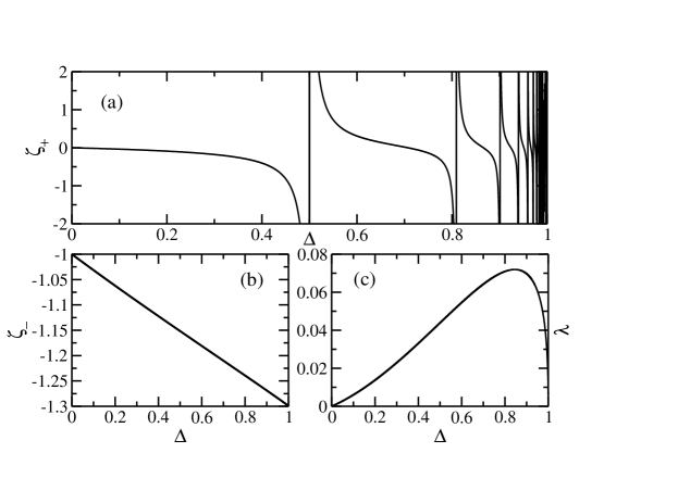
Figure 2: (a) $\zeta_{+}$ as function of anisotropy $\Delta$. The amplitude diverges whenever the argument of the $\tan$-function in Eq. (55) is $\pm\pi/2(\mbox{mod}\,2\pi)$. (b) $\zeta_{-}$, and (c) $\lambda$, Eq. (48) as a function of $\Delta$.

5.2.2 The finite field case

For a finite magnetic field ($B<\infty$), the Bethe ansatz integral equation cannot be solved analytically. However the amplitudes $\eta_{\pm}$ can be related to changes in the Luttinger parameter and velocity when changing the field.[38, 30] This allows for an accurate numerical determination of these parameters.

The basic idea is again quite simple. We consider the Luttinger liquid Hamiltonian at some finite magnetic field $h_{0}$. This means that our left and right modes live near Fermi points $\pm k_{F}\neq\pm\pi/2$. Now we apply an additional small magnetic field $\delta h$ which we can take care of by the boson shift (34). If we now calculate the free energy we obtain

$$f=-\frac{\pi T^{2}}{6v(h)}-\underbrace{\frac{K(h)}{2\pi v(h)}}_{=\chi(h)/2}(J\delta h)^{2}$$ (56)

with $h=h_{0}+\delta h$. The interaction parameters $K(h)$ and $v(h)$ can be determined numerically as described in Sec. 4. Now we can expand (56) in $\delta h$ and obtain to lowest order

$$\delta f=\frac{\pi T^{2}}{6v^{2}(h_{0})}\frac{\partial v}{\partial h}\bigg{|}_{h=h_{0}}\delta h;\quad\delta\chi=\frac{K(h_{0})}{\pi v(h_{0})}\left[\frac{1}{K}\frac{\partial K}{\partial h}\bigg{|}_{h=h_{0}}-\frac{1}{v}\frac{\partial v}{\partial h}\bigg{|}_{h=h_{0}}\right]\delta h$$ (57)

These corrections have to stem from the dimension three operators (27). The second approach therefore is to keep $K=K(h=h_{0})$, $v=v(h=h_{0})$ fixed and to perform the shift (34) also in (27). Calculating again the free energy by standard techniques we now find

$$\delta f=\left(3\eta_{-}-\eta_{+}\right)\frac{\pi\,\sqrt{K}J\delta h\,T^{2}}{18v^{3}(h_{0})}+(\eta_{-}-\eta_{+})\,\frac{K^{3/2}\left(J\delta h\right)^{3}}{6\pi v^{3}(h_{0})};\quad\delta\chi=(\eta_{+}-\eta_{-})\frac{K^{3/2}J}{\pi v^{3}(h_{0})}\delta h$$ (58)

A comparison of (57) and (58) yields two equations from which one obtains[38, 30]

$$\eta_{-}=\frac{v}{K^{1/2}}\frac{\partial v}{\partial h}+\frac{v^{2}}{2K^{3/2}}\frac{\partial K}{\partial h},\qquad\eta_{+}=\frac{3v^{2}}{2K^{3/2}}\frac{\partial K}{\partial h}.$$ (59)

From this result a few general conclusions can be drawn. For a free model, $\eta_{+}$ should vanish because a mixing of right and left movers is then impossible. This is indeed the case since $K$ does not change when applying a field in this case. Furthermore, $\eta_{+}$ will also be absent for models such as the Calogero-Sutherland model where $K$ remains independent of the applied field even in the interacting case. The $\eta_{-}$-term, on the other hand, is already present in a non-interacting system due to band curvature with $\eta_{-}=M^{-1}$ for $\Delta=0$. The result (59) of course also agrees with the expansion for small $\Delta$, Eq. (28).

The parameters $\eta_{\pm}$ are shown in Fig. 3 for different anisotropies $\Delta$ as a function of magnetization $m$.

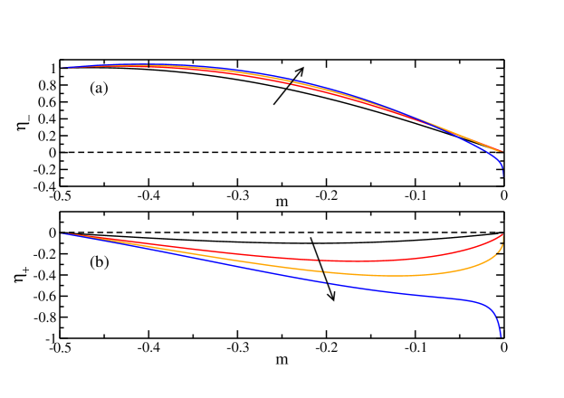
Figure 3: (a) $\eta_{-}$ as a function of magnetization $m$ for $\Delta=0.2,0.5,0.7,0.9$ (in arrow direction). (b) Same for $\eta_{+}$. Note that $\eta_{\pm}\to-\infty$ for $m\to 0$ in the case $\Delta=0.9$ leading to a sign change of $\eta_{-}$.

While $\eta_{\pm}\to 0$ for $m\to 0$ if $K>5/8$ as expected from the weak coupling expansion (28) both parameters diverge, on the other hand, for $K<5/8$ ($\Delta>\cos(\pi/5)\approx 0.81$). This behavior is discussed in more detail in Ref. 14 and we remind the reader that divergencies also occur in the amplitude $\zeta_{+}$ for $h=0$.

6 Applications

We now want to consider a few examples where the low-energy effective theory has been used to obtain parameter-free results for several important observables.

6.1 Impurities, Friedel oscillations and nuclear magnetic resonance

One of the best known realizations of the spin-$1/2$ antiferromagnetic Heisenberg chain is the cuprate Sr₂CuO₃.[6] In this system excess oxygen dopes holes into the chain which seem to be basically immobile.[7, 40] Effectively, this leads to randomly distributed non-magnetic impurities which cut the spin chain into finite segments. The magnetic properties are therefore determined by an ensemble of finite chains of random length $N$ with OBC.

In a chain with OBC, translational invariance is broken leading to a position dependent local susceptibility

$$\chi_{j}=\frac{\partial}{\partial h}\langle S^{z}_{j}\rangle_{h=0}=\frac{1}{T}\langle S^{z}_{j}S^{z}_{\rm tot}\rangle_{h=0}$$ (60)

where $T$ is the temperature and $S^{z}_{\rm tot}=\sum_{j}S^{z}_{j}$. In order to calculate $\chi_{j}$ in the low-energy limit, we can express the spin operator in terms of the bosonic field

$$S^{z}_{j}\approx\sqrt{\frac{K}{\pi}}\partial_{x}\Phi+c(-1)^{j}\cos\sqrt{4\pi K}\Phi\;.$$ (61)

Here the prefactor of the uniform part is fixed by the condition $\sum_{j}S^{z}_{j}=S^{z}_{\rm tot}$.[29, 4] The amplitude of the alternating part, on the other hand, can be fixed with the help of the Bethe ansatz solution. The techniques required are, however, much more involved than the ones reviewed in the previous section. In particular, one finds that $c=\sqrt{A_{z}/2}$ with $A_{z}$ as given in Eq. (4.3) of Ref. 34.

Using Eq. (61) we can write $\chi_{j}=\chi^{\rm uni}+(-1)^{j}\chi_{j}^{\rm st}$. The uniform part $\chi^{\rm uni}$ for the Luttinger model is given by

$$\chi^{\rm uni}=-\frac{\partial^{2}f}{\partial h^{2}}\bigg{|}_{h=0}=\frac{1}{LT}\frac{\sum_{S_{z}}S_{z}^{2}\exp\left[-\frac{\pi v}{2KLT}S_{z}^{2}\right]}{\sum_{S_{z}}\exp\left[-\frac{\pi v}{2KLT}S_{z}^{2}\right]}\,.$$ (62)

For $LT/v\to 0$ and $L$ even $\chi_{s}\sim\frac{2}{LT}\exp\left[-\frac{\pi v}{2KLT}\right]$ whereas for $L$ odd $\chi_{s}\sim(4LT)^{-1}$. For $LT/v\to\infty$ the thermodynamic limit result (35) is recovered. Note that this zeroth order result is position independent and shows scaling with $LT$. Corrections to scaling occur due to the irrelevant bulk and boundary operators. For $0\leq\Delta\leq 1$ the leading bulk irrelevant operator is due to Umklapp scattering (31). This leads to a first order correction in the free energy

$$\delta f_{1}=\frac{\lambda}{L}\int_{0}^{L}dx\langle\cos(4\sqrt{\pi K}\phi)\rangle_{S_{z}}\exp(-8\pi K\langle\phi\phi\rangle_{\rm osc})$$ (63)

where we have used the mode expansion for OBC

$$\phi(x,t) = \sqrt{\frac{\pi}{16K}}+\sqrt{\frac{\pi}{K}}S^{z}_{\rm tot}\frac{x}{L}+\sum_{n=1}^{\infty}\frac{\sin\left(\pi nx/L\right)}{\sqrt{\pi n}}\left(\mbox{e}^{-i\pi n\frac{vt}{L}}a_{n}+\mbox{e}^{i\pi n\frac{vt}{L}}a_{n}^{\dagger}\right)$$ (64)

to split the expectation value of the Umklapp operator into an $S_{z}$ (zero mode) and an oscillator part. Furthermore, we have used the cumulant theorem for the oscillator part. It is now straightforward, although a bit tedious, to evaluate the two parts of (63). From this the correction to the uniform part of the susceptibility in first order in Umklapp scattering can readily be obtained. [11]

The boundary operator (32) yields a further correction[11]

$$\delta\chi^{\rm uni}_{2}=\frac{\pi vb}{2KT^{2}L^{3}}\left[\frac{\sum_{S_{z}}S_{z}^{4}\mbox{e}^{-\frac{\pi vS_{z}^{2}}{2KLT}}}{\sum_{S_{z}}\mbox{e}^{-\frac{\pi vS_{z}^{2}}{2KLT}}}-\frac{\left(\sum_{S_{z}}S_{z}^{2}\mbox{e}^{-\frac{\pi vS_{z}^{2}}{2KLT}}\right)^{2}}{\left(\sum_{S_{z}}\mbox{e}^{-\frac{\pi vS_{z}^{2}}{2KLT}}\right)^{2}}\right]\,.$$ (65)

In the thermodynamic limit, Eq. (65) reduces to $\delta\chi^{\rm uni}_{2}\to Kb/(\pi vL)$. The field theory result in this limit can be compared with the calculation of the boundary susceptibility based on the Bethe ansatz [32, 33] and the proportionality constant $b$ can be fixed

$$b=2^{-1/2}\sin\left[\pi K/(4K-2)\right]/\cos\left[\pi/(8K-4)\right]\;.$$ (66)

To first order in Umklapp scattering and in the dimension three boundary operator a parameter-free result for $\chi^{\rm uni}$ can therefore be obtained.

The alternating part of the susceptibility (60) can be written as $\chi_{j}^{\rm st}=\frac{c}{T}\exp(-2\pi K\langle\phi\phi\rangle_{\rm osc})\langle\cos\sqrt{4\pi K}\phi\rangle_{S_{z}}$ where we have again split the correlation function into an oscillator and a zero mode part using the mode expansion. The calculation is now completely analogous to the calculation of the correction (63) leading to

$$\chi_{j}^{\rm st}=-\left(\frac{\pi}{N+1}\right)^{K}\!\!\!\!\!\!\frac{\eta^{3K}\left(\mbox{e}^{-\frac{\pi v}{TL}}\right)}{\theta_{1}^{K}\left(\frac{\pi j}{N+1},\mbox{e}^{-\frac{\pi v}{2TL}}\right)}\frac{\sum_{m}m\sin[2\pi mj/(N+1)]\mbox{e}^{-\pi vm^{2}/(2KLT)}}{\sum_{m}\mbox{e}^{-\pi vm^{2}/(2KLT)}}.$$ (67)

Here $\eta(q)$ is the Dedekind eta-function, and $\theta_{1}(u,q)$ the elliptic theta function of the first kind. In the thermodynamic limit, $L=Na\to\infty$, where we have reintroduced the lattice constant $a$ for clarity, we can simplify our result and obtain

$$\chi_{j}^{\rm st}=\frac{2cK}{v}\frac{x}{\left[\frac{v}{\pi T}\sinh\left(\frac{2\pi Tx}{v}\right)\right]^{K}}$$ (68)

with $x=ja$. This agrees for the isotropic Heisenberg case, $K=1/2$, with the result in Ref. 41. In Fig. 4 the parameter-free formula for $\chi_{j}=\chi^{\rm uni}+(-1)^{j}\chi_{j}^{\rm st}$ is compared to Quantum-Monte-Carlo data.[12]

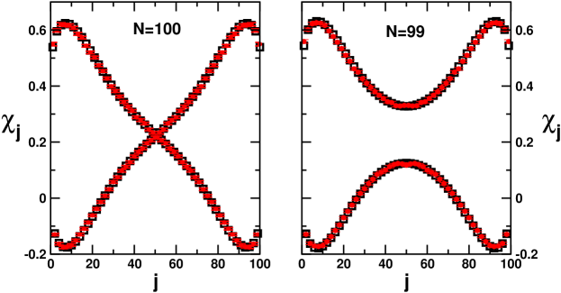
Figure 4: Local susceptibility for a finite open $XXZ$ chain with length $N$, $\Delta=0.3$ at temperature $T/J=0.02$. The squares denote the result of the parameter-free field theory formula, the circles are results obtained by Quantum Monte Carlo calculations.[12]

The position dependent susceptibility is directly measured as Knight shift in NMR. The hyperfine interaction couples nuclear and electron spins and the Knight shift of the nuclear resonance frequency for a chain segment of length $N$ is given by $K^{(N)}_{j}=(\gamma_{e}/\gamma_{n})\sum_{j^{\prime}}A^{j-j^{\prime}}\chi^{(N)}_{j^{\prime}}$, where $\gamma_{e}$ ($\gamma_{n}$) is the electron (nuclear) gyromagnetic ratio, respectively. The hyperfine interaction is short ranged so that usually only $A^{0}$ and $A^{\pm 1}$ matter. For a random distribution of non-magnetic impurities within a chain the NMR spectrum reflects the distribution of Knight shifts for an ensemble of spin chains with random lengths. This leads to rather complicated NMR spectra[7, 40] whose properties can be fully understood using the parameter-free results for the susceptibility discussed above.[12]

6.2 The spin-lattice relaxation rate and transport

The spin current (or particle current in the fermionic language) for the $XXZ$ model is defined by

$$\mathcal{J}=-\frac{iJ}{2}\sum_{l}\left(S^{+}_{l}S^{-}_{l+1}-S^{+}_{l+1}S^{-}_{l}\right)\approx-\sqrt{\frac{K}{\pi}}\int dx\,\partial_{x}\theta$$ (69)

Whether or not the integrable $XXZ$ model supports ballistic transport at finite temperatures has been the topic of a long-standing debate.[20, 42, 43, 44, 13, 14] As discussed in Sec. 2.1 ballistic transport is signalled by a non-zero Drude weight and related to the part of the current which cannot decay due to conservation laws, see Eq. (7). For finite magnetic field, the Mazur inequality indeed immediately yields a non-zero Drude weight.[20] In this case the conserved energy current (52) becomes

$$\tilde{\mathcal{J}}^{E}_{0}=-v^{2}\int dx\,\partial_{x}\theta\,\partial_{x}\phi-hv\sqrt{\frac{K}{\pi}}\int dx\,\partial_{x}\theta=\mathcal{J}^{E}_{0}+h\mathcal{J}$$ (70)

where we have used again the shift in the boson field, Eq. (34). The equal time correlations in (7) can now be evaluated for the Luttinger model (25) and[14]

$$D\geq D_{\rm Mazur}=\frac{1}{2TL}\frac{\langle\mathcal{J}\tilde{\mathcal{J}}^{E}_{0}\rangle^{2}}{\langle(\tilde{\mathcal{J}}^{E}_{0})^{2}\rangle}=\frac{vK/2\pi}{1+\frac{\pi^{2}}{3K}\left(\frac{T}{h}\right)^{2}}\qquad(T,h\ll J).$$ (71)

For $T/h\to 0$ the Mazur bound obtained from the overlap with $\tilde{\mathcal{J}^{E}_{0}}$ saturates the exact zero temperature Drude weight $D(T=0)=vK/2\pi$ [45]. Furthermore, one can also use the Bethe ansatz to calculate the Mazur bound $D_{\rm Mazur}$ exactly. The obtained result agrees with (71) up to temperatures of order $J$.[14]

For zero magnetic field, however, the overlap between all local conserved quantities $\mathcal{Q}_{n}$ of the $XXZ$ model which can be constructed from the transfer matrix (4) and the current $\mathcal{J}$ vanishes, because the $\mathcal{Q}_{n}$ are even under particle-hole transformations while $\mathcal{J}$ is odd. Recently, a quantity—not related to the conserved quantities obtained from the Bethe ansatz solution—has been constructed for an open $XXZ$ chain which is conserved up to boundary terms.[46] This quantity seems to protect part of the current in the thermodynamic limit, a view which appears to be supported by new numerical data.[47] As in the finite field case, the correct picture therefore seems to be that at finite temperatures a diffusive and a ballistic transport channel coexist.[13] For temperatures $T/J\in[0.2,0.5]$ and $h=0$, the Drude weight, however, seems to be much suppressed compared to its zero temperature value known exactly from Bethe ansatz. Furthermore, the Drude weight seems to vanish completely at finite temperatures in the isotropic case, $\Delta=1$. We therefore ignore a protected part of the current for now and first concentrate on the diffusive channel. The corrections due to a possible conserved part of the current are discussed at the end of this section.

From an experimental point of view, it is of great interest to understand the intrinsic mechanism which leads to spin diffusion in the $XXZ$ model. Spin diffusion has directly been observed in the spin lattice relaxation rate $1/T_{1}$ measured in NMR experiments as a magnetic field dependence $1/T_{1}\sim 1/\sqrt{h}$.[8, 48] Both the spin lattice relaxation rate and the conductivity can be calculated within the Luttinger model from the retarded boson propagator

$$\langle\phi\phi\rangle^{\rm ret}(q,\omega)=\frac{v}{\omega^{2}-v^{2}q^{2}-\Pi^{\rm ret}(q,\omega)}.$$ (72)

For $\Pi^{\rm ret}(q,\omega)=0$ this is just the free boson propagator. In the zero field case, the leading irrelevant operator is the Umklapp term (31) and we will concentrate here on calculating the self-energy $\Pi^{\rm ret}(q,\omega)$ in first order in this perturbation. Further contributions to the self-energy will stem from the band curvature terms and are discussed in Ref. 14. Note, however, that only Umklapp scattering can give the bosons a finite lifetime and thus lead to diffusive transport. The calculation of the correlation function (72) in first order in Umklapp scattering is straightforward.[49] We find[13, 14]

$$\Pi^{\rm ret}(q,\omega)\approx-2i\gamma\omega$$ (73)

where the decay rate $\gamma$ is given by

$$2\gamma=8\pi K\lambda^{2}\sin(4\pi K)\left(\frac{2\pi}{v}\right)^{8K-2}\!\!\!\!\!\!\!\Gamma(1/2-2K)\Gamma(2K)\frac{B(2K,1-4K)}{\sqrt{\pi}2^{4K+1}}\cot(2\pi K)T^{8K-3}$$ (74)

in the anisotropic case and by

$$2\gamma=\pi g^{2}T$$ (75)

in the isotropic case, $\Delta=1$. The running coupling constant $g=g(T)$ is determined by (49). The Kubo formula directly relates the conductivity $\sigma(q,\omega)$ to the calculated bosonic Green’s function

$$\sigma(q,\omega)=\frac{K}{\pi}\text{i}\omega\langle\phi\phi\rangle^{ret}(q,\omega)$$ (76)

and due to the finite relaxation rate $\gamma$ at finite temperatures one find a Lorentzian for the real part of the conductivity

$$\sigma^{\prime}(q=0,\omega)=\frac{vK}{\pi}\frac{2\gamma}{\omega^{2}+(2\gamma)^{2}}.$$ (77)

At the same time, also the spin lattice relaxation rate can be expressed by the same bosonic Green’s function

$$\frac{1}{T_{1}}\approx-\frac{2KT}{\pi\omega_{e}}\int\frac{q^{2}dq}{2\pi}\,|A(q)|^{2}\,\textrm{Im }\langle\phi\phi\rangle_{\rm ret}(q,\omega_{e}).$$ (78)

Here $\omega_{e}=\mu_{B}h$ is the electron magnetic resonance frequency.[14] If the hyperfine coupling form factor $A(q)$ picks out the $q\sim 0$ contributions of the integral (78) as in the oxygen NMR experiment on Sr₂CuO₃ in Ref. 8 then $1/T_{1}$ and the conductivity $\sigma^{\prime}(q\sim 0,\omega)$ are directly related. The experimentally considered spin chains are almost isotropic, $\Delta\approx 1$. Using the parameter-free result (75) we obtain the diffusive behavior

$$\frac{1}{T_{1}T}\sim\sqrt{\frac{\gamma(T)}{\omega_{e}}}\sim\sqrt{\frac{T/\ln^{2}(J/T)}{\omega_{e}}}.$$ (79)

The only free parameters remaining depend on microscopic details of the considered compound. Both the exchange constant $J$ and the hyperfine coupling constant $A(q)$ can be fixed by analyzing the susceptibility and performing a $K-\chi$ analysis respectively.[6, 8, 40] Integrability therefore makes it possible to obtain an analytical result for the spin-lattice relaxation rate which includes the intrinsic relaxation processes. The comparison of the result (79) with experiment as shown in Fig. 5 demonstrates that Umklapp scattering seems to be the dominant source for relaxation and that other contributions, e.g., due to electron-phonon scattering are small.

Figure 5: Spin-lattice relaxation rate $1/T_{1}$ for Sr₂CuO₃. Experimental data (symbols) are compared to the field theoretical result. The only free parameters are the exchange constant $J\sim 1800$ K and the hyperfine coupling tensor which have been determined experimentally. A more detailed analysis is presented in Ref. 14.

Finally, we have to discuss the possible conservation of part of the current even at zero magnetic field. The quantity constructed in Ref. 46 contains terms active over several lattice sites for $0<\Delta<1$. It is therefore non-trivial to bosonize this term and to consider the consequences of its (almost) conservation for the low-energy effective theory in a similar spirit to our discussion of $J^{E}$ in Sec. 5.2. An alternative method discussed in Refs. 50, 13, 14 is to use a memory matrix formalism to calculate the self-energy (72) in the presence of conservation laws. Instead of Eq. (73) the self-energy then reads

$$\Pi(q=0,\omega)\approx\frac{-2i\gamma\omega}{1+2i\gamma y/\omega}\quad\mbox{with}\quad y=\frac{\langle\mathcal{J}Q\rangle^{2}}{\langle\mathcal{J}^{2}\rangle\langle Q^{2}\rangle-\langle\mathcal{J}Q\rangle^{2}}$$ (80)

where $Q$ is the conserved quantity with $\langle\mathcal{J}Q\rangle\neq 0$. As a consequence, the current-current correlation function at large times is now given by

$$\frac{1}{L}\langle\mathcal{J}(t)\mathcal{J}\rangle=\frac{KvT}{\pi(1+y)}\left[y+\exp(-2\gamma(1+y)t)\right]$$ (81)

where the first term is proportional to the Drude weight and the second term describes the diffusive part. For $\Delta=1$ the Drude weight seems to be zero at finite temperatures[46] so that our theoretical analysis of $1/T_{1}$ is not affected. In any case, the spin chains in Sr₂CuO₃ do not represent an integrable system and there is therefore certainly no ballistic channel. It is known, for example, that in this compound also a weak next-nearest neighbor coupling $J_{2}\sim 0.1J$ exists. While this coupling destroys integrability it will only lead to a weak renormalization of the Umklapp amplitude $\lambda$.[29] It is thus legitimate to use the results for the integrable model to analyze the experimental data for $1/T_{1}$.

7 Conclusions

Integrable gapless one-dimensional quantum models allow to test many predictions of Luttinger liquid theory. As such they have been vital in confirming the universal applicability of the latter. On the other hand, Luttinger liquid theory has also helped to understand integrable quantum models better. Except for the simplest integrable systems, such as free bosonic or fermionic particles and to some extent also Calogero-Sutherland type models, an exact calculation of correlation functions for arbitrary distances and times has not been achieved yet. A combination of Luttinger liquid theory and integrability then often allows to obtain a more complete picture. For Bethe ansatz integrable systems such as the Lieb-Liniger Bose gas, the (anisotropic) Heisenberg, the Hubbard, or the supersymmetric $t-J$ model it is possible to fix the velocity of the collective excitations $v$ and the Luttinger parameter $K$ as a function of density and interaction strength. For the Luttinger model, (dynamical) correlations can then be easily calculated.

Often one can go even one step further and determine the amplitudes of leading irrelevant operators acting as corrections to the Luttinger Hamiltonian as well as amplitudes of correlation functions, exactly. This article is by no means a complete review of all the results which have been obtained in this field. Instead, I have used the $XXZ$ model as an example and have summarized how $v$, $K$ as well as the amplitudes of the leading irrelevant band curvature terms and Umklapp scattering can be determined. As an application, I have shown that this allows to derive parameter-free results for the local susceptibility in open Heisenberg chains and quantitatively explains Knight shift spectra which have been investigated by nuclear magnetic resonance for compounds such as Sr₂CuO₃. As a second application, I have presented results for the relaxation rate of the Luttinger liquid bosons at finite temperatures in first order in Umklapp scattering. From this a parameter-free formula for the spin-lattice relaxation rate $1/T_{1}$ can be obtained which is in excellent agreement with experiment. The same bosonic correlation function and the same relaxation rate determine, on the other hand, also the particle transport. In general, the $XXZ$ model has coexisting ballistic and diffusive transport channels. The relative weight of each of these channels can be determined by combining the Luttinger model—keeping the dangerously irrelevant Umklapp term with known amplitude—with a memory-matrix calculation.

There are many more interesting results which have not been covered in this review. One of the perhaps most fascinating recent developments is the so-called non-linear Luttinger liquid theory which allows to calculate dynamic response functions while taking band curvature into account.[51] This has lead to the discovery of new power laws near edge singularities. For integrable models the exponents of these power laws can be determined exactly.[52] A comprehensive overview about these developments has been given in a recent excellent review.[53]

References

- [1] J. M. Luttinger, J. Math. Phys. 4, 1154 (1963).
- [2] D. C. Mattis and E. H. Lieb, J. Math. Phys. 6, 304 (1965).
- [3] A. Luther and I. Peschel, Phys. Rev. B 12, 3908 (1975).
- [4] T. Giamarchi, Quantum physics in One Dimension, Clarendon Press, Oxford, (2004).
- [5] L. Onsager, Phys. Rev. 65, 117 (1944).
- [6] N. Motoyama, H. Eisaki, and S. Uchida, Phys. Rev. Lett. 76, 3212 (1996).
- [7] M. Takigawa, N. Motoyama, H. Eisaki, and S. Uchida, Phys. Rev. B 55, 14129 (1997).
- [8] K. R. Thurber, A. W. Hunt, T. Imai, and F. C. Chou, Phys. Rev. Lett. 87, 247202 (2001).
- [9] S. Eggert, Phys. Rev. B 53, 5116 (1996).
- [10] J. Sirker, N. Laflorencie, S. Fujimoto, S. Eggert, and I. Affleck, Phys. Rev. Lett. 98, 137205 (2007).
- [11] J. Sirker, N. Laflorencie, S. Fujimoto, S. Eggert, and I. Affleck, J. Stat. Mech. P02015 (2008).
- [12] J. Sirker and N. Laflorencie, Europhys. Lett. 86, 57004 (2009).
- [13] J. Sirker, R. G. Pereira, and I. Affleck, Phys. Rev. Lett. 103, 216602 (2009).
- [14] J. Sirker, R. G. Pereira, and I. Affleck, Phys. Rev. B 83, 035115 (2011).
- [15] E. H. Lieb and W. Liniger, Phys. Rev. 130, 1605 (1963).
- [16] T. Kinoshita, T. Wenger, and D. S. Weiss, Nature 440, 900 (2006).
- [17] C. N. Yang and C. P. Yang, Phys. Rev. 150, 321 (1966).
- [18] J.-S. Caux and J. Mossel, J. Stat. Mech. P02023 (2011).
- [19] F. H. L. Essler, H. Frahm, F. Göhmann, A. Klümper, and V. E. Korepin, The One-Dimensional Hubbard model, Cambridge University Press, Cambridge, (2005).
- [20] X. Zotos, F. Naef, and P. Prelovšek, Phys. Rev. B 55, 11029 (1997).
- [21] P. Mazur, Physica 43, 533 (1969).
- [22] M. Suzuki, Physica 51, 277 (1971).
- [23] P. Jung and A. Rosch, Phys. Rev. B 75, 245104 (2007).
- [24] J. M. Deutsch, Phys. Rev. A 43, 2046 (1991).
- [25] H. Bethe, Z. Phys. 71, 205 (1931).
- [26] E. K. Sklyanin, J. Phys. A 21, 2375 (1988).
- [27] F. C. Alcaraz, M. N. Barber, M. T. Batchelor, R. J. Baxter, and G. R. W. Quispel, J. Phys. A 20, 6397 (1987).
- [28] M. Takahashi, Thermodynamics of one-dimensional solvable problems, Cambridge University Press, (1999).
- [29] S. Eggert and I. Affleck, Phys. Rev. B 46, 10866 (1992).
- [30] R. G. Pereira, J. Sirker, J.-S. Caux, R. Hagemans, J. M. Maillet, S. R. White, and I. Affleck, J. Stat. Mech. P08022 (2007).
- [31] S. Lukyanov, Nucl. Phys. B 522, 533 (1998).
- [32] M. Bortz and J. Sirker, J. Phys. A: Math. Gen. 38, 5957 (2005).
- [33] J. Sirker and M. Bortz, J. Stat. Mech. P01007 (2006).
- [34] S. Lukyanov and V. Terras, Nucl. Phys. B 654, 323 (2003).
- [35] N. Kitanine, J. M. Maillet, and V. Terras, Nucl. Phys. B 554, 647 (1999).
- [36] N. Kitanine, J. M. Maillet, and V. Terras, Nucl. Phys. B 567, 554 (2000).
- [37] N. Kitanine, K. K. Kozlowski, J. M. Maillet, V. A. Slavnov, and V. Terras, J. Stat. Mech. P05028 (2011).
- [38] R. G. Pereira, J. Sirker, J.-S. Caux, R. Hagemans, J. M. Maillet, S. R. White, and I. Affleck, Phys. Rev. Lett. 96, 257202 (2006).
- [39] S. Fujimoto and S. Eggert, Phys. Rev. Lett. 92, 037206 (2004).
- [40] J. P. Boucher and M. Takigawa, Phys. Rev. B 62, 367 (2000).
- [41] S. Eggert and I. Affleck, Phys. Rev. Lett. 75, 934 (1995).
- [42] J. V. Alvarez and C. Gros, Phys. Rev. Lett. 88, 077203 (2002).
- [43] X. Zotos, Phys. Rev. Lett. 82, 1764 (1999).
- [44] F. Heidrich-Meisner, A. Honecker, D. C. Cabra, and W. Brenig, Phys. Rev. B 66, 140406(R) (2002).
- [45] B. S. Shastry and B. Sutherland, Phys. Rev. Lett. 65, 243 (1990).
- [46] T. Prosen, Phys. Rev. Lett. 106, 217206 (2011).
- [47] C. Karrasch, J. H. Bardarson, and J. E. Moore, Phys. Rev. Lett. 108, 227206 (2012).
- [48] F. L. Pratt, S. J. Blundell, T. Lancaster, C. Baines, and S. Takagi, Phys. Rev. Lett. 96, 247203 (2006).
- [49] M. Oshikawa and I. Affleck, Phys. Rev. B 65, 134410 (2002).
- [50] A. Rosch and N. Andrei, Phys. Rev. Lett. 85, 1092 (2000).
- [51] A. Imambekov and L. I. Glazman, Science 323, 228 (2009).
- [52] R. G. Pereira, S. R. White, and I. Affleck, Phys. Rev. Lett. 100, 027206 (2008).
- [53] A. Imambekov, T. L. Schmidt, and L. I. Glazman, arXiv:1110.1374 (2011).