Capillary buckling of a thin film adhering to a sphere

Abstract

We present a combined theoretical and experimental study of the buckling of a thin film wrapped around a sphere under the action of capillary forces. A rigid sphere is coated with a wetting liquid, and then wrapped by a thin film into an initially cylindrical shape. The equilibrium of this cylindrical shape is governed by the antagonistic effects of elasticity and capillarity: elasticity tends to keep the film developable while capillarity tends to curve it in both directions so as to maximize the area of contact with the sphere. In the experiments, the contact area between the film and the sphere has cylindrical symmetry when the sphere radius is small, but destabilises to a non-symmetric, wrinkled configuration when the radius is larger than a critical value. We combine the Donnell equations for near-cylindrical shells to include a unilateral constraint with the impenetrable sphere, and the capillary forces acting along a moving edge. A non-linear solution describing the axisymmetric configuration of the film is derived. A linear stability analysis is then presented, which successfully captures the wrinkling instability, the symmetry of the unstable mode, the instability threshold and the critical wavelength. The motion of the free boundary at the edge of the region of contact, which has an effect on the instability, is treated without any approximation.

1 Introduction

The buckling of thin plates has been studied for a long time, both theoretically [1, 2] and experimentally [3]. Initially, the main motivation was to avoid loads associated with catastrophic failure modes. Recent research efforts on thin plates and shells have been driven by technological applications involving thinner and thinner plates [4], by the idea that controlled buckling can provide useful functionality [5], and by strongly non-linear phenomena appearing far above the bifurcation threshold [6]. The wrinkling of a semi-infinite elastic medium under finite compression, known as Biot’s problem [7, 8], as well as the buckling of a thin stiff film coated to a compliant substrate [9, 10, 11] are just two examples of classical problems in mechanical engineering whose non-linear aspects have been well understood only recently. We refer the reader to [12] for a comprehensive review.

When the adhesion between a thin film under residual compression and a thick substrate is relatively weak, buckling can take place along with delamination, resulting in the formation of blisters [13, 14]. Buckling-driven delamination can lead to various patterns which are affected both by the mode-mixity [15], i. e. the dependence of the interfacial energy on the loading mode, and by the irreversibility of the interfacial fracture [16]. In recent experiments, a simpler variant of the classical delamination problem has been proposed, whereby the adhesion between the film and the substrate is provided by capillary forces arising from a thin liquid bridge [17, 18]: capillary forces are reversible and act like a self-healing interface crack. These experiments can be done at the centimeter scale.

In the present paper, we study some buckling patterns produced by these experiments. Specifically, we consider the case of the capillary adhesion between a thin elastic film and a doubly-curved substrate. This geometry has been considered by one of us in a recent experimental paper [18]. It built up on previous work addressing the related case of a spherical shell adhering onto a planar substrate [19, 20, 21]. In our experiments, a rigid spherical cap is first coated by a wetting liquid and a thin polypropylene film is then applied onto it. As it wraps the sphere under the action of capillary forces, the film is forced to stretch by Gauss’ theorema egregium [22]. Stretching allows it to make up for the mismatch of Gaussian curvature, which is zero in the planar film and non-zero along the spherical substrate. This leads to a variety of adhesion morphologies, as shown in figure 1, where the contact region varies from a simple band to complex branched patterns.

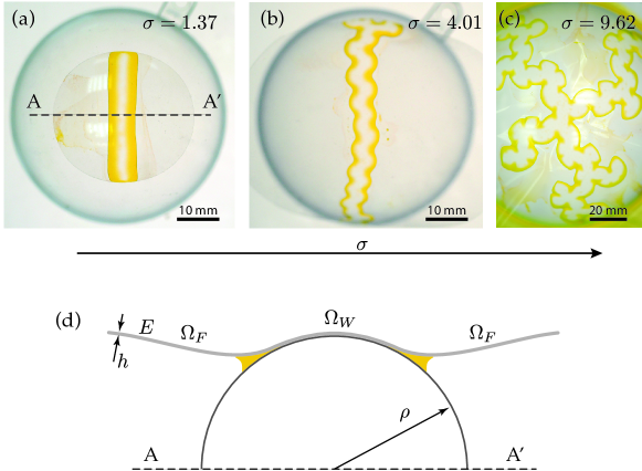
Figure 1: Thin elastic films of thickness $h$, Young’s modulus $E$ and Poisson’s ratio $\nu$ are placed onto rigid spherical caps of radius $\rho$ coated with a wetting liquid, with surface tension $\gamma=22.4\mathrm{mN.m^{-1}}$. The liquid has been dyed in yellow to help visualization: the yellow region are the liquid meniscus. Note that the interior of the region of contact appear uncolored as there is almost no fluid there. Top view of three different experiments: (a) $E=2.8\,\mathrm{GPa}$, $h=30\,\mu$m, $\rho=25\,$mm (b) $E=2.6\,\mathrm{GPa}$, $h=15\,\mu$m, $\rho=25\,$mm (c) $E=2.6\,\mathrm{GPa}$, $h=15\,\mu$m, $\rho=60\,$mm. The parameter $\sigma$, defined in equation (19), measures the strength of adhesion relative to the stiffness of the film. (d) Sketch of a cut through a vertical plane $\mathrm{AA}^{\prime}$.

In reference [18], one of us studied the antagonistic effects of elasticity and capillarity using order of magnitude arguments, and proposed an estimate for the size of the region of adhesion which successfully compares to the experiments.

Here, we study these patterns quantitatively. In particular we address the transition shown in the figure, whereby a band-like region of contact with straight edges (figure 1a) bifurcates into a sinuous pattern with undulatory edges (figure 1b) when the adhesion becomes stronger or the film becomes thinner. This is interpreted as a buckling bifurcation caused by compressive stress along the straight edges. We carry out a stability analysis based on the classical Donnell equations for nearly-cylindrical shells, modified to account for the effect of adhesion. The motion of the free boundary at the edge of the region of contact is considered without any approximation.

The paper is organized as follows. In section 2, we derive the equations for a nearly-cylindrical elastic shell adhering to a sphere, with an emphasis on the equilibrium conditions along the edge of the moving contact region. In section 3, we derive a non-linear solution to these equations relevant to the unbuckled configuration with cylindrical symmetry. These results are compared to experimental data. In section 4, we then study the linear stability of the cylindrical solution. The predictions regarding the symmetry of the buckling modes, their wavelength and the critical loads are compared to experimental data in section 5.

2 Governing equations: Donnell’s shell equations with adhesion

The Donnell-Mushtari-Vlasov equations for nearly-cylindrical shells, simply called the Donnell equations thereafter, are derived by combining the general equations for shells undergoing finite displacements with specific scaling assumptions for the magnitude of the displacement. Even though the Donnell equations have been known and used for a long time, this derivation is useful as it highlights the simple assumptions that underlie them. More importantly, the variational framework that is used to derive the Donnell equations allows us to include adhesion and the presence of a moving boundary in a natural and consistent manner.

2.1 Geometry

The reference configuration considered here is shown in figure 2a.

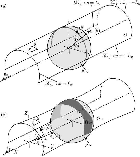
Figure 2: (a) The reference configuration: the cylindrical shell makes tangent contact with the sphere along the great circle $x=0$. (b) A typical deformed configuration: the region of contact $\Omega_{W}$, shown in dark grey, is bounded by two curves $G_{-}$ and $G_{+}$.

A thin cylindrical shell $\Omega$ of half-length $L_{x}$, half-width $L_{y}$, thickness $h$ and radius $\rho$ rests tangentially to a sphere of radius $\rho$. The Lagrangian coordinates along the shell are denoted by $x$ and $y=\rho\,\theta$, where $\theta$ is the azimuthal angle in the reference configuration. Let $\partial\Omega_{x}^{\pm}$ and $\partial\Omega_{y}^{\pm}$ correspond to the edges of the shell at $x=\pm L_{x}$ and $y=\pm L_{y}$, respectively. We assume that the shell is made of an isotropic linear elastic material with Young’s modulus $E$ and Poisson’s ratio $\nu$.

A typical deformed configuration is shown in figure 2b. The displacement of the middle surface of the shell is denoted $u_{x}(x,y)$, $u_{y}(x,y)$ and $w(x,y)$, where the first two functions are the tangential components of the displacement, and $w(x,y)$ is the radial displacement (deflection), counted positive towards the exterior of the shell. In the deformed configuration, the position of a generic point lying on the center-surface of the shell reads

$$\underline{\tilde{x}}(x,y) =\Big{(}x+u_{x}(x,y)\Big{)}\,\underline{e}_{x}+\Big{(}\rho+w(x,y)\Big{)}\,\underline{e}_{1}(\tilde{\theta}(x,y))\textrm{,}$$ (1a)

where the azimuthal angle in deformed configuration reads

$$\quad\tilde{\theta}(x,y) =\frac{y+u_{y}(x,y)}{\rho}\textrm{.}$$ (1b)

Here $\underline{e}_{1}(\tilde{\theta})=(0,\cos\tilde{\theta},\sin\tilde{\theta})$ is the radial unit vector in the plane perpendicular to the axis $\underline{e}_{x}$.

The purely radial displacement $w_{s}\leq 0$ that brings a point from the cylindrical reference configuration onto the sphere is such that $x^{2}+(\rho+w_{s}(x))^{2}=\rho^{2}$, and so

$$w_{s}(x)=-(\rho-\sqrt{\rho^{2}-x^{2}})$$

where $x$ is the axial coordinate and $r$ is the radial coordinate. In the following, we shall use a second-order approximation, valid for $|x|\ll\rho$,

$$w_{s}(x)=-\frac{1}{2}\,\frac{x^{2}}{\rho}\textrm{.}$$ (2)

In this approximation, the sphere has been effectively replaced by its osculating paraboloid. The non-penetration condition is then expressed as a unilateral constraint,

$$w(x)\geq w_{s}(x)\textrm{.}$$ (3)

We denote $\Omega_{W}$ the contact zone between the sphere and the shell, and $\Omega_{F}$ the free part of the shell, $\Omega=\Omega_{W}\cup\Omega_{F}$. Neglecting the width of the meniscus, we assume that the boundary $G=\Omega_{W}\cap\Omega_{F}$ between the two domains is made up of two curves,

$$G=G_{-}\cup G_{+}\textrm{.}$$ (4)

In addition, we assume that each one of this curve is a graph,

$$G_{-} =\{(x,y)\;|\;x=g_{-}(y)\}$$ (5)

$$G_{+} =\{(x,y)\;|\;x=g_{+}(y)\}\textrm{.}$$ (6)

This assumption is valid for configurations that are close to an axisymmetric configuration, for which both the functions $g_{-}$ and $g_{+}$ are constant. The wet region $\Omega_{W}$ lies inside the boundaries $G_{-}$ and $G_{+}$ and the free region $\Omega_{F}$ lies outside,

$$\Omega_{W} =\{(x,y)\;|\;g_{-}(x)\leq x\leq g_{+}(y)\}$$ (7)

$$\Omega_{F} =\{(x,y)\;|\;x\leq g_{-}(y)\textrm{ or }g_{+}(y)\leq x\}\textrm{.}$$ (8)

In the rest of the paper, Greek indices such as $\alpha$ or $\beta$ represent the Lagrangian coordinates, $\alpha=x$ or $\alpha=y$, and follow the implicit summation convention for repeated indices.

2.2 Scaling assumptions

Before introducing the fundamental mechanical quantities, which are the membrane strain $e_{\alpha\beta}$, the curvature strain $b_{\alpha\beta}$, the membrane stress $n_{\alpha\beta}$ and the bending moment $m_{\alpha\beta}$, we present the scaling assumptions that underlie the Donnell equations.

First, the thin-shell theory assumes that the following slenderness parameter is small,

$$\eta^{2}=\frac{h}{\sqrt{12}\,\rho}\textrm{.}$$ (9)

We shall therefore consider the limit

$$\eta\ll 1\textrm{.}$$ (10)

The Donnell equations assume that the shell remains close to the cylindrical configuration of reference. How close depends on the small parameter $\eta$: as shown in A, it is natural to rescale the deflection by $\rho\,\eta^{2}$, in-plane lengths by $\rho\,\eta$, and in-plane displacements by $\rho\,\eta^{3}$. Therefore, we define rescaled lengths by

$$\overline{x}=\frac{x}{\rho\,\eta}\qquad\qquad\overline{y}=\frac{y}{\rho\,\eta},$$ (11a)

and the rescaled displacement by

$$\overline{u}_{\alpha}(\overline{x},\overline{y}) =\frac{1}{\rho\,\eta^{3}}\,u_{\alpha}(x,y),$$ (11b)

$$\overline{w}(\overline{x},\overline{y}) =\frac{1}{\rho\,\eta^{2}}\,w(x,y)\textrm{.}$$ (11c)

The parabolic approximation of the sphere profile in equation (2) reads, in dimensionless variables,

$$\overline{w}_{\mathrm{s}}(\overline{x})=-\frac{1}{2}\overline{x}^{2}\textrm{.}$$ (12)

Note that the assumption under which this approximation has been derived, $|x|\ll\rho$ is consistent with the new scales introduced here: when $\overline{x}$ is of order 1 (and in fact, as long as it remains smaller than the large number $\eta^{-1}$), then $|x|\ll\rho$ and the sphere is indeed well approximated by its osculating paraboloid.

For the sake of consistency, we rescale the membrane strain $e_{\alpha\beta}$ by $\eta^{2}$, the curvature strain $b_{\alpha\beta}$ by $1/\rho$, the membrane stress $n_{\alpha\beta}$ by $C\,\eta^{2}$ and the bending moment $m_{\alpha\beta}$ by $B/\rho$, where $B=Eh^{3}/[12(1-\nu^{2})]$ and $C=Eh/(1-\nu^{2})$ denote the bending and stretching moduli of the shell, respectively. This is written

$$\overline{e}_{\alpha\beta}(\overline{x},\overline{y}) =\frac{1}{\eta^{2}}\,e_{\alpha\beta}(x,y)$$ (13a)

$$\overline{b}_{\alpha\beta}(\overline{x},\overline{y}) =\rho\,b_{\alpha\beta}(x,y)$$ (13b)

$$\overline{n}_{\alpha\beta}(\overline{x},\overline{y}) =\frac{1}{C\,\eta^{2}}\,n_{\alpha\beta}(x,y)$$ (13c)

$$\overline{m}_{\alpha\beta}(\overline{x},\overline{y}) =\frac{\rho}{B}\,m_{\alpha\beta}(x,y)\emph{.}$$ (13d)

The definition of the small parameter $\eta$ given earlier in eq. (9) warrants that the bending energy density $\frac{1}{2}\,m_{\alpha\beta}\,b_{\alpha\beta}$ and the stretching energy density $\frac{1}{2}\,n_{\alpha\beta}\,e_{\alpha\beta}$ are commensurate when $\eta$ goes to zero.

2.3 Membrane and curvature strains

From now on, we shall use dimensionless quantities everywhere, and drop bars to easy legibility. The above scaling assumptions allow one to simplify the expressions for the membrane and curvatures strains from the general theory of shells as follows,

$$e_{\alpha\beta}(x,y) =\left(\frac{u_{\alpha,\beta}(x,y)+u_{\beta,\alpha}(x,y)}{2}+\delta_{\alpha y}\,\delta_{\beta y}\,w(x,y)\right)+\frac{1}{2}\,w_{,\alpha}(x,y)\,w_{,\beta}(x,y)$$ (14a)

$$b_{\alpha\beta}(x,y) =-w_{,\alpha\beta}(x,y)\textrm{.}$$ (14b)

These expressions are shown to derive from the scaling assumptions in A. Here we use the Kronecker delta symbol, which is defined by

$$\delta_{\alpha\beta}=\begin{cases}1&\text{if }\alpha=\beta\\ 0&\text{if }\alpha\neq\beta\end{cases}$$ (15)

and use commas in indices to denote partial derivatives, as in the expression

$$u_{x,y}(x,y)=\frac{\partial u_{x}(x,y)}{\partial y}\textrm{.}$$

The strain approximation in equation (14a) is at the heart of Donnell’s model for nearly-cylindrical shells, and has been used by numerous authors, see for instance [23]. Only the non-linear terms that are important near the onset of buckling have been retained.

2.4 Constitutive law and energy

The shell’s material is assumed to be linearly elastic and isotropic. The Hookean constitutive laws read:

$$n_{\alpha\beta}(x,y) =(1-\nu)\,e_{\alpha\beta}(x,y)+\nu\,\delta_{\alpha\beta}\,\big{(}\operatorname{tr}\underline{\underline{e}}(x,y)\big{)}$$ (16a)

$$m_{\alpha\beta}(x,y) =(1-\nu)\,b_{\alpha\beta}(x,y)+\nu\,\delta_{\alpha\beta}\,\big{(}\operatorname{tr}\underline{\underline{b}}(x,y)\big{)}$$ (16b)

This is a rescaled form of the original constitutive laws given in the Appendix in equation (91). Thanks to our rescalings in equation (13), the stretching and bending moduli have effectively been set to one.

In the experiments, the fim is naturally planar and is bent into a cylindrical shape by the action of capillary forces. By contrast, the constitutive equation (16b) describes a naturally cylindrical shell with natural radius $\rho$: the bending moment $m_{\alpha\beta}$ is zero when the bending strain $\underline{\underline{b}}$ cancels, which happens in the configuration of reference. The case of a naturally planar film could be treated by modifying bending strain, replacing $\underline{\underline{b}}$ with $(\underline{\underline{b}}+\kappa_{0}\,\underline{e}_{y}\otimes\underline{e}_{y})$ everywhere, where $\kappa_{0}=-1/\rho$ is the curvature strain in reference configuration. As we shall see later, only the derivatives of the bending moment enter into the local equations of equilibrium. As a result, $\kappa_{0}$ is absent from these equations, and only affects boundary layers near the free edges. To simplify the analysis of these boundaries, we ignore this and set $\kappa_{0}=0$. This is a valid approximation for the entire pattern, except very close to the film boundaries.

The linear constitutive laws correspond to the following quadratic elastic energy,

$$E_{shell}=\iint_{\Omega}\frac{1}{2}\,(n_{\alpha\beta}\,e_{\alpha\beta}+m_{\alpha\beta}\,b_{\alpha\beta})\;\mathrm{d}x\,\mathrm{d}y$$ (17)

which is the sum of a stretching and a bending term.

The adhesion between the shell and the rigid sphere is modelled by an energy $(2\gamma)$ per unit area of the contact region. Indeed the liquid perfectly wets both the shell and the rigid sphere, and any increase in the area of contact removes two air/liquid interfaces, each having an energy $\gamma$ per unit area [24], where $\gamma$ is the surface tension of the liquid.

The rescaled adhesion energy thus reads:

$$E_{adhesion}=-\iint_{\Omega}2\,\sigma^{2}\,\chi_{W}(G;x,y)\,\mathrm{d}x\,\mathrm{d}y\textrm{,}$$ (18)

where $\chi_{W}(G;x,y)$ is the characteristic function of the wet domain: $\chi_{W}(G;x,y)=1$ in the wet region $(x,y)\in\Omega_{W}$, and $\chi_{W}(G;x,y)=0$ in the free region. The coefficient $\sigma^{2}$ is the capillary energy rescaled by the typical energy per unit area introduced earlier, $B/\rho^{2}$:

$$\sigma^{2}=\frac{\gamma}{B/\rho^{2}}=\left(\frac{\rho}{L_{ec}}\right)^{2}\textrm{.}$$ (19)

Here we have introduced the elastocapillary length [24],

$$L_{ec}=\sqrt{\frac{B}{\gamma}}=\sqrt{\frac{E\,h^{3}}{12\,(1-\nu^{2})\,\gamma}}\textrm{,}$$ (20)

which arises from a balance of the bending rigidity of the shell $B$ and the adhesion energy $\gamma$. At length scales smaller than $L_{ec}$, bending stiffness dominates capillary effects. The elastocapillary length sets the typical radius of the sphere beyond which adhesion is possible, as noted in reference [18].

2.5 Constraints and boundary conditions

In the wet region, the condition of contact with the sphere reads:

$$w(x,y)=w_{\mathrm{s}}(x)\quad\textrm{in }\Omega_{\mathrm{w}}\textrm{,}$$ (21)

where $w_{\mathrm{s}}$ is the parabolic approximation of the deflection of the rigid sphere derived in equation (12). We assume that the contact is frictionless.

We consider that the shell is infinitely long in its $y$ direction. This is captured by the following boundary condition on the remote edges $\partial\Omega_{y}^{\pm}$:

$$u_{y}(x,L_{y}^{\pm})=V^{\pm}$$ (22)

where the two unknown scalars $V^{+}$ and $V^{-}$ denote an unknown rigid-body motion of the edges consistent with the symmetry. They will be determined later by a condition of equilibrium of the boundary. This boundary condition means that the remote edges $\partial\Omega_{y}^{\pm}$ remain contained in a plane passing through the $X$ axis, even though this plane can freely rotate about this axis to accommodate an average extension or contraction of the shell in its $y$ direction. In the experiments, the film has a finite extent, and the above boundary condition is relevant to the case where its size is much larger than the wavelength of the instability: anticipating the notations of section 4, this writes $L_{y}\gg 2\pi/k_{\mathrm{c}}$.

Finally, we introduce a new set of variables $(q_{x},q_{y})$ which is the local slope of the shell with respect to the mobile frame,

$$q_{\alpha}(x,y)=w_{,\alpha}(x,y)$$ (23)

In the following, these $q_{\alpha}$’s will be considered variables independent from the deflection $w$, and the equation (23) just written will be viewed as a constraint. This allows our second-order variational problem to be written as a first-order one having additional variables and constraints, and simplifies the derivation of the equilibrium equations.

The Lagrangian of our constrained minimization problem is formed by augmenting the elastic and adhesion energies in equations (17) and (18) with the constraints in equations (21), (22) and (23) by means of Lagrange multipliers, denoted $\pi(x,y)$, $\nu^{\pm}(x)$ and $\lambda_{\alpha}(x,y)$:

$$E_{tot}(u_{\alpha},w,q_{\alpha},V^{\pm},G,\pi,\nu^{\pm},\lambda_{\alpha})=\\ \iint_{\Omega}\frac{1}{2}\,(n_{\alpha\beta}\,e_{\alpha\beta}+m_{\alpha\beta}\,b_{\alpha\beta})\,\mathrm{d}x\,\mathrm{d}y-\iint_{\Omega}2\,\sigma^{2}\,\chi_{W}(G)\,\mathrm{d}x\,\mathrm{d}y\\ -\iint_{\Omega}\pi\,(w-w_{s})\,\chi_{W}(G)\,\mathrm{d}x\,\mathrm{d}y-\sum_{s=\pm}\int_{\partial\Omega_{y}^{s}}\nu^{s}\,(u_{y}-V^{s})\,\mathrm{d}x-\iint_{\Omega}\lambda_{\alpha}\,(w_{,\alpha}-q_{\alpha})\,\mathrm{d}x\,\mathrm{d}y\textrm{.}$$ (24)

The interpretation of the Lagrange multipliers just introduced will be given in section 2.6. Note that the constraints (22) on the boundaries $\partial\Omega_{y}^{-}$ and $\partial\Omega_{y}^{+}$ are taken care of using a summation over the values $s=-$ and $s=+$.

2.6 Equations of equilibrium

In this section, we derive the equilibrium equations and the boundary conditions using variational calculus, by cancelling the first variation of the Lagrangian just written. This yields the classical Donnell equations for shells inside each domain $\Omega_{W}$ and $\Omega_{F}$, as well as boundary conditions, including an adhesion condition at the interface $G$ between the wet and free regions.

We first compute the variation of the Lagrangian with respect to the unknowns $(u_{\alpha},w,q_{\alpha},V^{\pm},\pi,\nu^{\pm},\lambda_{\alpha})$ considering that domains $\Omega_{W}$ and $\Omega_{F}$ and their boundary $G$ remain fixed, as expressed by the notation $\delta g=0$,

$$\delta E_{tot}^{{\dagger}}=\delta E_{tot}(\delta u_{\alpha},\delta w,\delta q_{\alpha},\delta V^{\pm},\delta g_{\pm}=0,\delta\pi,\delta\nu^{\pm},\delta\lambda_{\alpha})=\\ \iint_{\Omega}(n_{\alpha\beta}\,\delta e_{\alpha\beta}+m_{\alpha\beta}\,\delta b_{\alpha\beta})\;\mathrm{d}x\,\mathrm{d}y-\iint_{\Omega}\pi\,\chi_{W}(G)\,\delta w\;\mathrm{d}x\,\mathrm{d}y\\ -\sum_{s=\pm}\int_{\partial\Omega_{y}^{s}}\,\nu^{s}\,\delta u_{y}\;\mathrm{d}x+\sum_{s=\pm}\left(\int_{\partial\Omega_{y}^{s}}\nu^{s}\;\mathrm{d}x\right)\,\delta V^{s}-\iint_{\Omega}\lambda_{\alpha}\,(\delta w_{,\alpha}-\delta q_{\alpha})\,\mathrm{d}x\,\mathrm{d}y\\ -\iint_{\Omega}(w-w_{s})\,\chi_{W}(G)\,\delta\pi\;\mathrm{d}x\,\mathrm{d}y-\sum_{s=\pm}\int_{\partial\Omega_{y}^{s}}(u_{y}-V^{s})\,\delta\nu^{s}\;\mathrm{d}x-\iint_{\Omega}(w_{,\alpha}-q_{\alpha})\,\delta\lambda_{\alpha}\;\mathrm{d}x\,\mathrm{d}y$$ (25)

where we use the fact that $\delta(n_{\alpha\beta}\,e_{\alpha\beta})=2\,n_{\alpha\beta}\,\delta e_{\alpha\beta}$ and $\delta(m_{\alpha\beta}\,b_{\alpha\beta})=2\,m_{\alpha\beta}\,\delta b_{\alpha\beta}$, as we assume linear constitutive laws. The three last terms, which come from the variation with respect to the Lagrange multipliers $(\pi,\nu^{\pm},\lambda_{\alpha})$, enforce the kinematic relations in equations (21), (22), (23), as expected.

The complementary variations with respect to the position of the boundary $G$ will be computed later, with the help of B. They yield jump conditions across the boundary, which include the condition of adhesion.

Calculating the first variation of the strain defined in equation (14), and using the symmetry of the stress tensors $n_{\alpha\beta}$ and $m_{\alpha\beta}$, we have $n_{\alpha\beta}\,\delta e_{\alpha\beta}=n_{\alpha\beta}\,(\delta u_{\alpha,\beta}+\delta_{\alpha y}\,\delta_{\beta y}\,\delta w+w_{\beta}\,\delta w_{,\alpha})$ and $m_{\alpha\beta}\,\delta b_{\alpha\beta}=-m_{\alpha\beta}\,\delta q_{\alpha,\beta}$. Note that the symbol $\delta$ without any subscript denotes the variation of a function, while $\delta_{\alpha\beta}$ with subscripts is the Kronecker delta symbol introduced in equation (15). Integrating by parts and grouping the terms, we have:

$$\delta E_{tot}^{{\dagger}}=-\iint_{\Omega}\Big{(}\big{[}n_{\alpha\beta,\beta}\big{]}\,\delta u_{\alpha}+\big{[}\pi\,\chi_{W}(G)+(n_{\alpha\beta}\,w_{,\alpha})_{,\beta}-n_{yy}-\lambda_{\alpha,\alpha}\big{]}\,\delta w+\big{[}-m_{\alpha\beta,\beta}-\lambda_{\alpha}\big{]}\,\delta q_{\alpha}\Big{)}\,\mathrm{d}x\,\mathrm{d}y\\ \\ +\int_{\partial\Omega}\Big{(}\big{[}n_{\alpha\beta}-\delta_{\alpha y}\,\sum_{s=\pm}\nu^{s}\,\chi_{\partial\Omega_{y}^{s}}\,\big{]}\,\delta u_{\alpha}+\big{[}n_{\alpha\beta}\,w_{,\alpha}-\lambda_{\beta}\big{]}\,\delta w-\big{[}m_{\alpha\beta}\big{]}\,\delta q_{\alpha}\Big{)}\,N_{\beta}\,\mathrm{d}\ell+\sum_{s=\pm}\left(\int_{\partial\Omega_{y}^{s}}\nu^{s}\,\mathrm{d}x\right)\,\delta V^{s}$$ (26)

where we denote the entire lateral boundary by $\partial\Omega=\partial\Omega_{x}^{\pm}\cup\partial\Omega_{y}^{\pm}$, the element of length along the lateral boundary by $\mathrm{d}\ell=\mathrm{d}x$ on $\partial\Omega_{y}^{\pm}$ and $\mathrm{d}\ell=\mathrm{d}y$ on $\partial\Omega_{x}^{\pm}$. In addition, $\underline{N}=(N_{x},N_{y})$ stands for the normal to a boundary $\partial\Omega$, $\underline{N}$ being oriented towards the exterior of the domain $\Omega$.

The equilibrium condition, $\delta E_{tot}^{{\dagger}}=0$, yields the following equations on $\Omega$:

$$n_{\alpha\beta,\beta}(x,y) =0$$ (27a)

$$m_{\alpha\beta,\alpha\beta}(x,y)+n_{\alpha\beta}(x,y)\,w_{,\alpha\beta}(x,y)-n_{yy}(x,y)+\chi_{W}(G;x,y)\,\pi(x,y) =0\textrm{.}$$ (27b)

Here we have replaced the shear force $\lambda_{\alpha}$ by its expression $\lambda_{\alpha}=-m_{\alpha\beta,\beta}$. The latter comes from the condition associated with perturbations $\delta q_{\alpha}$.

The equations (27) are the Donnell equations for thin cylindrical shells, see for instance [23]. The first equation (27a) is a tangential balance of forces. The second equation (27b) is a transverse balance of force. The Lagrange multiplier $\pi$ can be interpreted as the pressure of contact with the sphere in the wet region. The equation (27b) allows one to compute the contact pressure $\pi(x,y)$ in the wet region where $w=w_{s}$ is known; in the free region, the pressure term $\pi(x,y)$ is zero and the equation is an equation for the unknown deflection $w(x,y)$.

On the lateral boundary $\partial\Omega_{x}^{\pm}$, we recover the natural boundary conditions for a plate or shell with a free edge, see for instance [25],

$$n_{\alpha x}(\pm L_{x},y) =0$$ (28a)

$$m_{xx}(\pm L_{x},y) =0$$ (28b)

$$m_{xx,x}(\pm L_{x},y)+2\,m_{xy,y}(\pm L_{x},y) =0\textrm{.}$$ (28c)

Note that equation (28c) comes from the integration by parts of $\delta q_{y}$ in equation (26), as $\delta q_{y}=(\delta w)_{,y}$ on $\partial\Omega_{x}^{\pm}$.

On the other lateral boundaries $\partial\Omega_{y}^{\pm}$, the boundary conditions read:

$$n_{xy}(x,\pm L_{y}) =0$$ (29a)

$$n_{yy}(x,\pm L_{y}) =\nu^{\pm}(x)$$ (29b)

$$m_{yy}(x,\pm L_{y}) =0$$ (29c)

$$m_{yy,y}(x,\pm L_{y})+2\,m_{xy,x}(x,\pm L_{y}) =-\nu^{\pm}(x)w_{,y}(x,\pm L_{y})$$ (29d)

$$\int_{\partial\Omega_{y}^{\pm}}n_{yy}(x,\pm L_{y})\,\mathrm{d}x =0\textrm{.}$$ (29e)

Here we used again the fact $\delta q_{x}=(\delta w)_{,x}$ on $\partial\Omega_{y}^{\pm}$. The Lagrange multiplier $\nu^{\pm}$ can be interpreted as the normal stress on $\partial\Omega_{y}^{\pm}$. The equation (29e) expresses the fact that no average force is applied on the shell in the $y$ direction (natural boundary condition).

2.7 Equations for the moving boundary

We recall the general expression of the corner conditions in a two-dimension domain in B, known as the Weierstrass-Erdmann conditions. They yield the jump conditions at the moving interface between two subdomains, in any minimization problem where the contributions to the objective function have different expressions in each subdomain. This applies to the Lagrangian of our problem in equation (24), which can indeed be written as

$$E_{tot}=\iint_{\Omega_{W}}\mathcal{L}^{W}(u_{\alpha},w,q_{\alpha},\pi,\lambda_{\alpha})\,\mathrm{d}x\,\mathrm{d}y+\iint_{\Omega_{F}}\mathcal{L}^{F}(u_{\alpha},w,q_{\alpha},\pi,\lambda_{\alpha})\,\mathrm{d}x\,\mathrm{d}y+\int_{\partial\Omega}\cdots\,\mathrm{d}\ell\textrm{.}$$ (30)

The integrands have different expressions in the free and wet regions,

$$\mathcal{L}^{F}(u_{\alpha},w,q_{\alpha},\pi,\lambda_{\alpha};x,y) =\frac{1}{2}\,(n_{\alpha\beta}\,e_{\alpha\beta}+m_{\alpha\beta}\,b_{\alpha\beta})-\lambda_{\alpha}\,(w_{,\alpha}-q_{\alpha})$$ (31)

$$\mathcal{L}^{W}(u_{\alpha},w,q_{\alpha},\pi,\lambda_{\alpha};x,y) =\mathcal{L}^{F}(u_{\alpha},w,q_{\alpha},\pi,\lambda_{\alpha})-2\,\sigma^{2}-\pi\,(w-w_{\mathrm{s}})\emph{.}$$ (32)

These notations conform with those of equation (96) in B. As usual with shell models having non-zero bending rigidity, the tangent displacement $u_{\alpha}(x,y)$ is required to be continuous, and the transverse displacement $w(x,y)$ to be $\mathcal{C}^{1}$-smooth. In particular, across the boundary $G$, we have

$$[\![u_{\alpha}]\!] =0$$ (33a)

$$[\![w]\!] =0$$ (33b)

$$[\![w_{,\alpha}]\!] =0\textrm{,}$$ (33c)

where

$$[\![A]\!]=A^{F}(x_{G},y_{G})-A^{W}(x_{G},y_{G})$$ (34)

denotes the discontinuity of a function $A$ across a point $(x_{G},y_{G})$ lying on the boundary $G$.

By differentiation of the equalities (33) along the boundary $G$, we find

$$[\![u_{\alpha,T}]\!] =0$$ (35a)

$$[\![w_{,\alpha T}]\!] =0\textrm{,}$$ (35b)

where $\underline{T}=(T_{x},T_{y})$ is the unit tangent to $G$, and a $T$ in subscript denotes the tangent derivative $f_{,T}=T_{\alpha}\,f_{,\alpha}$. The functions $w$ and $q_{\alpha}=w_{,\alpha}$ have prescribed values in the wet region $\Omega_{W}$ but can take any value in the free region $\Omega_{F}$. By contrast, $u_{\alpha}$ is unconstrained in the entire domain $\Omega$.

Using the fact that the elastic energy is a quadratic form of the strain by equation (17) first, and using the definition of the strain in equation (14) next, one can compute the so-called generalized momentum and identify the result with the internal stress, up to a sign,

$$\frac{\partial\mathcal{L}^{i}}{\partial u_{\alpha,\beta}} =n_{\gamma\rho}^{i}\,\frac{\partial e_{\gamma\rho}}{\partial u_{\alpha,\beta}} =n_{\gamma\rho}^{i}\,\frac{1}{2}\,(\delta_{\alpha\gamma}\,\delta_{\beta\rho}+\delta_{\alpha\rho}\,\delta_{\beta\gamma}) =n_{\alpha\beta}^{i}$$ (36)

$$\frac{\partial\mathcal{L}^{i}}{\partial q_{\alpha,\beta}} =m_{\gamma\rho}^{i}\,\frac{\partial b_{\gamma\rho}}{\partial q_{\alpha,\beta}} =-m_{\gamma\rho}^{i}\,\frac{1}{2}\,(\delta_{\alpha\gamma}\,\delta_{\beta\rho}+\delta_{\alpha\rho}\,\delta_{\beta\gamma}) =-m_{\alpha\beta}^{i}$$ (37)

where $i=W,F$ is any of the wet (W) or free (F) region.

We now apply the corner conditions derived in B after identifying the regions $\Omega_{1}=\Omega_{W}$, $\Omega_{2}=\Omega_{F}$. The unknowns, collectively denoted $\xi_{\alpha}$ in the appendix, are the in-plane displacement $u_{\beta}$, the deflection $w$ and the slope $q_{\beta}$.

When the equilibrium condition (101) derived in the appendix is applied to the unknown $\xi_{\alpha}=u_{\alpha}$, we find $[\![n_{\alpha\beta}]\!]\,N_{\beta}=[\![n_{\alpha N}]\!]=0$ after using equation (36). Note that $N_{\beta}$ refers to the local normal vector, while $n_{\alpha\beta}$ refers to a generic component of the membrane stress. For $\alpha=T$ and $\alpha=N$ this yields $[\![n_{TN}]\!]=0$ and $[\![n_{NN}]\!]=0$, which are the classical conditions for the in-plane equilibrium of the boundary.

It turns out that the third independent component $n_{TT}$ of the membrane stress is also continuous across the boundary, even though this does not directly follow from equilibrium. To show this, let us write the constitutive law (16a) in dimensionless form, $n_{TT}=\nu\,n_{NN}+(1-\nu^{2})\,e_{TT}$. In the right-hand side, $n_{NN}$ is continuous as we have just shown, while $e_{TT}$ is continuous as a consequence of the smoothness conditions (33) and (35). Therefore, the tangential stress $n_{TT}$ is continuous as well. To sum up, we have shown that all components of the membrane stress are continuous,

$$[\![n_{\alpha\beta}]\!]=0\textrm{.}$$ (38)

Using the constitutive law for stretching in its inverted form, one shows that the membrane strain is continuous as well,

$$[\![e_{\alpha\beta}]\!]=0\textrm{.}$$ (39)

As a result, the density of stretching energy is continuous, $[\![\frac{1}{2}\,n_{\alpha\beta}\,e_{\alpha\beta}]\!]=0$.

The discontinuity in the energy density is therefore the sum of an adhesion term, which is present only in the wet part, and a discontinuity in bending energy,

$$[\![\mathcal{L}]\!]=\mathcal{L}^{F}-\mathcal{L}^{W}=2\,\sigma^{2}+\frac{1}{2}\,[\![m_{\alpha\beta}\,b_{\alpha\beta}]\!]\textrm{.}$$ (40)

Considering now the condition (102) for equilibrium of the boundary with respect to the variable $\xi_{\alpha}=q_{\alpha}=w_{,\alpha}$, we have

$$2\,\sigma^{2}+\frac{1}{2}\,[\![m_{\alpha\beta}\,b_{\alpha\beta}]\!]-m_{\gamma\beta}^{F}\,[\![b_{\gamma\beta^{\prime}}]\!]\,N_{\beta}\,N_{\beta^{\prime}}=0\textrm{.}$$ (41)

It is consistent to use this equation (102) as the value of $q_{\alpha}=w_{,\alpha}=w_{s,\alpha}$ is prescribed in the adhering region.

Upon insertion of the constitutive law first, and of the continuity relations for the curvature next, one can rewrite the second term of equation (41) as

$$\frac{1}{2}\,[\![m_{\alpha\beta}\,b_{\alpha\beta}]\!]=\frac{1}{2}\,[\![b_{NN}^{2}+b_{TT}^{2}+2\,\nu\,b_{TT}\,b_{NN}+2\,(1-\nu)\,b_{TN}^{2}]\!]\\ =\frac{1}{2}\,\left([\![b_{NN}^{2}]\!]+2\,\nu\,b_{TT}\,[\![b_{NN}]\!]\right)\textrm{.}$$ (42)

Note that only the $NN$-component of $b_{\alpha\beta}=-w_{,\alpha\beta}$ is possibly discontinuous. As a result, only the set of indices $\gamma=N$ and $\beta^{\prime}=N$ need be considered in the last term of (41). Using the constitutive law for bending (16b) again, we can rewrite this last term as follows,

$$-m_{\gamma\beta}^{F}\,[\![b_{\gamma\beta^{\prime}}]\!]\,N_{\beta}\,N_{\beta^{\prime}}=-(b_{NN}^{F}+\nu\,b_{TT})\,[\![b_{NN}]\!]\textrm{.}$$ (43)

Inserting the expressions (42) and (43) into the equilibrium condition (41), we find that the terms proportional to Poisson’s ratio cancel out:

$$2\,\sigma^{2}+\frac{1}{2}\,\left((b_{NN}^{F})^{2}-(b_{NN}^{W})^{2}\right)-b_{NN}^{F}\,\left(b_{NN}^{F}-b_{NN}^{W}\right)=0\textrm{.}$$ (44)

After using the definition of the jump operator in equation (34), this can be simplified as

$$2\,\sigma^{2}-\frac{1}{2}\,[\![b_{NN}]\!]^{2}=0\textrm{.}$$ (45)

By developing in the non-penetration condition in equation (3) in Taylor series up to second order, and by using the continuity of the deflection and the slope in equations (33), we have

$$w_{,NN}(x_{G},y_{G})\geq w_{s,NN}(x_{G},y_{G})\textrm{.}$$ (46)

In terms of curvature, this yields $b_{NN}^{F}(x_{G},y_{G})\leq b_{NN}^{W}(x_{G},y_{G})$, which we rewrite using the jump notation as

$$[\![b_{NN}]\!]\leq 0\textrm{.}$$ (47)

Thus, the equation (45) implies

$$[\![b_{NN}]\!]=-2\,\sigma\textrm{,}$$ (48)

as $\sigma$ is a positive number.

To sum up, there are seven independent continuity and jump relations that must be enforced at the moving interface $g$. They read

$$[\![u_{x}]\!]_{x=g(y)} =0$$ (49a)

$$[\![u_{y}]\!]_{x=g(y)} =0$$ (49b)

$$[\![w]\!]_{x=g(y)} =0$$ (49c)

$$[\![w_{,N}]\!]_{x=g(y)} =0$$ (49d)

$$[\![n_{TN}]\!]_{x=g(y)} =0$$ (49e)

$$[\![n_{NN}]\!]_{x=g(y)} =0$$ (49f)

$$[\![m_{NN}]\!]_{x=g(y)} =-2\,\sigma\textrm{.}$$ (49g)

Equation (48) comes from equation (49g) after using the constitutive law. The notation $x=g(y)$ emphasises the fact that the jump operator is defined on the boundary $G$ whose equation is $x=g_{\pm}(y)$. A term proportional to the perturbation $\delta g_{\pm}$ of the boundary will appear in these equations when we consider the linear stability later on. This perturbation $\delta g_{\pm}$ must be considered as the shape of the boundary may be affected by the buckling. It corresponds to the quantity $a_{1}$ introduced later.

The jump relation (49g) arising from adhesion has previously been derived in an effectively 1D (axisymmetric) case [26, 27], as well as for elastic plates [13, 28]. This equation (49g) is also known in the context of classical fracture mechanics, as the delamination of a thin film on a rigid substrate can be seen as the propagation of a crack along an interface [15]: the energy release rate $G$ per unit width of a film adhering on a curved substrate reads $G=\frac{[\![m_{NN}]\!]^{2}}{2B}$, and equation (49g) expresses from the balance of energy, $G=2\,\gamma$.

3 A non-linear solution for the unbuckled state

In this section we derive an axisymmetric solution to the equations derived in section 2. The wet region $\Omega_{W}$ is then a strip bounded by two symmetric circles with equation $x=g_{\pm}(y)$, where $g_{\pm}(y)=\pm a_{0}$. Here $a_{0}$ denotes half the width of the strip, and will determined later as a function of the adhesion number $\sigma$.

In the axisymmetric case, the displacement is of the form

$$u_{x}(x,y) =u_{x}^{0i}(x)$$ (50a)

$$u_{y}(x,y) =E_{0}\,y$$ (50b)

$$w(x,y) =w_{0}^{i}(x)\textrm{,}$$ (50c)

where the index $i$ denotes the region ($i=W$ if $|x|\leq a_{0}$ and $i=F$ if $|x|\geq a_{0}$), the symbol ‘$0$’ refers to the unbuckled axisymmetric state. The unknown constant $E_{0}$ measures the uniform hoop strain, and will be determined later. It is related to the unknown uniform tangent displacement $V^{\pm}$ at the edges $y=\pm L_{y}$ by $E_{0}=u_{y,y}=(V^{+}-V^{-})/(2\,L_{y})$. Imposing a linear dependence of $u_{y}$ on the azimuthal variable $y$ warrants that the hoop strain will be independent of $y$, as required by the symmetry.

We compute the membrane strains

$$e_{xx}^{0}(x,y) ={u_{x}^{0i}}^{\prime}(x)+\frac{1}{2}\,({w_{0}^{i}}^{\prime}(x))^{2}$$ (51a)

$$e_{xy}^{0}(x,y) =0$$ (51b)

$$e_{yy}^{0}(x,y) =E_{0}+w_{0}^{i}(x)\textrm{.}$$ (51c)

They are all independent of the coordinate $$y$$, as required by the symmetry. All bending strains are zero, except for the axial component

$$\underline{\underline{b}}^{0}(x,y)=b^{0}_{xx}\,\underline{e}_{x}\otimes\underline{e}_{x},\quad b^{0}_{xx}=-{w_{0}^{i}}^{\prime\prime}(x)\textrm{.}$$ (51d)

By the constitutive law for stretching we have $n_{xy}(x,y)=0$ and $n_{\alpha\beta,y}(x,y)=0$, as required by the symmetry. The equilibrium condition (27a) along the direction $x$ ($\alpha=x$ in this equation) implies that the stress $n_{xx}$ does not depend on $x$ either. By the boundary condition (28a), this quantity vanishes everywhere, $n_{xx}^{0}(x,y)=0$. In terms of the in-plane strain, this writes $e_{xx}+\nu\,e_{yy}=0$, an equation which will be useful to reconstruct the in-plane displacement $u_{x}^{0i}(x)$:

$${u_{x}^{0i}}^{\prime}(x)=-\frac{1}{2}({w_{0}^{i}}^{\prime}(x))^{2}-\nu\,w_{0}^{i}(x)-\nu\,E_{0}\textrm{.}$$ (52)

Elimination of $e_{xx}=-\nu\,e_{yy}$ from the constitutive relation (16a) yields the expression of the only non-zero stress component,

$$\underline{\underline{n}}^{0}(x,y)=n_{yy}^{0}\,\underline{e}_{y}\otimes\underline{e}_{y},\qquad n_{yy}^{0}=(1-\nu^{2})\,e^{0}_{yy}(x,y)=(1-\nu^{2})\,(E_{0}+w_{0}^{i}(x))\textrm{.}$$ (53)

In the wet region $|x|\leq a_{0}$, the contact condition reads

$$w^{W}_{0}(x)=w_{s}(x)=-\frac{1}{2}\,x^{2}\textrm{.}$$ (54)

The membrane stress there is then found by inserting this expression into equation (53), up to the constant $E_{0}$ that will be determined later. The in-plane displacement ${u_{x}^{0W}}(x)$ is found by integration of equation (52) with the initial condition ${u_{x}^{0W}}(0)=0$ imposed by the symmetry.

By symmetry, many term cancel in the equation (27b) for the transverse equilibrium in the free region $|x|\geq a_{0}$, which reads

$$\frac{1}{1-\nu^{2}}\,{w_{0}^{F}}^{\prime\prime\prime\prime}(x)+w_{0}^{F}(x)=-E_{0}\textrm{.}$$ (55)

We consider the case of a shell of infinite length in the $x$-direction, $L_{x}\to\infty$. This corresponds to the situation in the experiments where the length $L_{x}$ of the film is much larger than the width of the wet region, that is much larger than the typical in-plane length $\sqrt{\rho\,h}$ which we used to make lengths dimensionless. The generic solution of equation (55) that is bounded near $x\to\pm\infty$ reads

$$w^{F}_{0}(x)=-E_{0}+e^{\pm\frac{x}{x^{*}(\nu)}}\,\left(A_{1}\,\cos\frac{x}{x^{*}(\nu)}+A_{2}\,\sin\frac{x}{x^{*}(\nu)}\right)$$ (56)

where $A_{1}$ and $A_{2}$ are unknown amplitudes, and

$$x^{*}(\nu)=\left(\frac{4}{1-\nu^{2}}\right)^{1/4}$$ (57)

is a scaling factor applicable to in-plane lengths. This $x^{*}(\nu)$ is a known function of Poisson’s ratio.

In order to determine the four constants $(A_{1},A_{2},E_{0},a_{0})$, we use all the boundary conditions that are not automatically satisfied, namely the continuity conditions (49c) and (49d), the equilibrium condition for the average force along the $y$-direction (29e), and the jump condition (49g) depending on the adhesion number $\sigma$:

$$w_{0}^{F}(a_{0}) =w_{0}^{W}(a_{0})$$ (58a)

$${w_{0}^{F}}^{\prime}(a_{0}) ={w_{0}^{W}}^{\prime}(a_{0})$$ (58b)

$$\int_{0}^{+\infty}n^{0}_{yy}(x)\,\mathrm{d}x =0$$ (58c)

$$m_{xx}^{F}(a_{0}) =m_{xx}^{W}(a_{0})-2\,\sigma$$ (58d)

Even though some of the equations for the problem are non-linear, equations (58) happen to be linear with respect to the unknowns $A_{1}$, $A_{2}$ and $E_{0}$, when we make use of equations (53), (54) and (56). This leads to a set of linear equations whose coefficients depend non-linearly on their arguments,

$$\underline{\underline{M}}\left(\frac{a_{0}}{x^{*}(\nu)},\sigma\right)\cdot\underline{X}=\underline{0}$$ (59a)

where

$$\underline{X}=\Big{(}A_{1},A_{2},E_{0},{a_{0}}^{2}\Big{)}$$ (59b)

and

$$\underline{\underline{M}}\left(\hat{a}=\frac{a_{0}}{x^{*}(\nu)},\sigma\right)=\begin{pmatrix}e^{-\hat{a}}\,\cos\hat{a}&e^{-\hat{a}}\,\sin\hat{a}&-1&\frac{1}{2}\\ -e^{-\hat{a}}\,(\cos\hat{a}+\sin\hat{a})&e^{-\hat{a}}\,(\cos\hat{a}-\sin\hat{a})&0&\frac{1}{\hat{a}}\\ e^{-\hat{a}}\,(\cos\hat{a}-\sin\hat{a})&e^{-\hat{a}}\,(\cos\hat{a}+\sin\hat{a})&0&-\frac{\hat{a}}{3}\\ e^{-\hat{a}}\,\sin\hat{a}&-e^{-\hat{a}}\,\cos\hat{a}&0&\frac{1}{\hat{a}^{2}}\,\left(\frac{1}{2}+\sigma\right)\end{pmatrix}\textrm{.}$$ (59c)

A necessary condition for this linear system to have a solution is

$$\det\left(\underline{\underline{M}}\left(\frac{a_{0}}{x^{*}(\nu)},\sigma\right)\right)=0\textrm{.}$$ (60)

One can simplify the determinant of $\underline{\underline{M}}$ and rewrite this equation as

$$\frac{3+6\,\hat{a}+6\,\hat{a}^{2}+2\,\hat{a}^{3}}{6\,(1+\hat{a})}=\sigma,\quad\textrm{where }\hat{a}=\frac{a_{0}}{x^{*}(\nu)}$$ (61)

This implicit relation, plotted in fig. 3a,

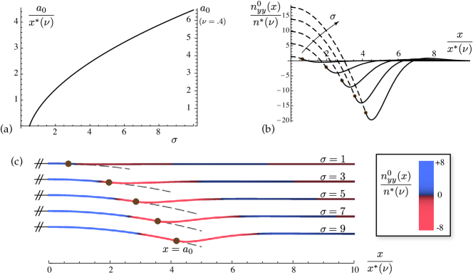
Figure 3: Axisymmetric solution. (a) Half-width of the band-like region of contact, as a function of the reduced adhesion $\sigma$. The vertical axis on the left-hand side shows the value of $a_{0}/x^{*}(\nu)$ which is independent of Poisson’s ratio, and that on the right-hand side shows the corresponding value of $a_{0}$ for the particular case $\nu=0.4$, as in the experiments. (b) Hoop stress $n_{yy}^{0}(x)/n^{*}(\nu)$, rescaled using $n^{*}(\nu)=1/(x^{*}(\nu))^{2}$, as a function of the rescaled axial coordinate $x/x^{*}(\nu)$, for increasing values of the adhesion $\sigma$. When expressed in these variables, the curves are independent of $\nu$. Dashed lines correspond to the wet region, solid lines to the free region. The different curves correspond to different values of adhesion, namely $\sigma=1,3,5,7$ and $9$. (c) Profile of the shell as obtained by cutting through a plane passing through the axis, for increasing values of the adhesion number $\sigma$. Only one half of the cut is shown, the entire profile being symmetric with respect to $x=0$. The profiles corresponding to different values of $\sigma$ have been offset vertically for clarity. As the adhesion $\sigma$ increases, the width of the region of contact increases, and the hoop stress becomes more and more compressive around the edge of the region of contact. This points to the existence of an instability, which is studied next.

selects the half-width $a_{0}=(x^{*}(\nu)\,\hat{a})$ of the region of contact $\Omega^{W}$ in the axisymmetric configuration, as a function of the dimensionless adhesion number $\sigma$. Note that this half-width $a_{0}$ goes to zero as $\sigma$ decreases to the value $1/2$: the adhering solution disappears when the adhesion is too weak, $\sigma<1/2$.

From now on, we assume $\sigma\geq 1/2$ and consider the value of $a_{0}$ that is the unique solution to equation (61). Then, the matrix in equation (59a) is singular and the solutions $\underline{X}$ of the linear system span a line. Generically, there is a unique vector $\underline{X}$ whose last component equals the square of the quantity $a_{0}$ just found, as imposed by equation (59b). The other components of this particular vector $\underline{X}$ set the values of the unknowns $A_{1}$, $A_{2}$ and $E_{0}$. For any value of the adhesion parameter $\sigma\geq 1/2$ this defines a unique axisymmetric solution. Some of these solutions are represented in figure 3c, for particular values of $\sigma$. The residual stress $\underline{\underline{n}}^{0}(x)$ given by equation (53) is plotted in figures 3b and c. We note that this residual hoop stress is compressive near the edge of the region of contact, as the film is pulled towards the axis by the adhesion.

In figure 4, we compare the prediction for the width of the contact region in equation (61) to the experimental data taken from Ref. [18], with no adjustable parameter.

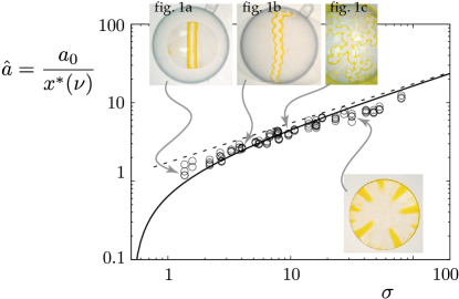
Figure 4: Size of the contact zone as a function of the adhesion parameter $\sigma$. Circular symbols correspond to experimental data from Ref. [18]. The solid line corresponds to the prediction of equation (61), and the dashed line to the asymptotic behaviour of equation (61). As the solid curve comes from the analysis on the unbuckled stated, it cannot be expected to be accurate far above threshold, when $\sigma$ becomes larger than $\sim 10$; a good agreement is observed nevertheless.

We find a good agreement. Interestingly, the agreement is good even in the post-buckled regime (when $\sigma$ is larger than approximately $5$), if we measure $a_{0}$ in the experiments as half the average strip width; this is unexpected as the present solution is not applicable above the bifurcation threshold.

In the limit of strong adhesion, when $\sigma$ is large, the half-width $a_{0}$ predicted by equation (61) becomes large as well, and is given asymptotically by $a_{0}=\sqrt{3\,\sigma}\,x^{*}(\nu)$. Restoring the physical units, this yields

$$a_{0}\approx\sqrt{6}\,\rho\,\left(\frac{\gamma}{Eh}\right)^{1/4}\emph{.}$$ (62)

We recover the scaling form proposed and verified in reference [18], and have obtained the value of the coefficient in addition.

We have derived a family of non-linear solution of the Donnell equations analytically that describe unbuckled, axisymmetric shapes of the film. The equations are non-linear and it is remarkable that these solutions can be derived without approximation. There is a unique axisymmetric solution when the adhesion is large enough, $\sigma\geq 1/2$. For lower adhesion, $\sigma<1/2$ no axisymmetric solution with extended contact can be found.

4 Stability analysis

Given the presence of compressive hoop stress in the axisymmetric solution shown in figure 3c, the neighborhood of the edges of the region of contact can become unstable, especially when the adhesion number $\sigma$ becomes large. Making use of the explicit solution for the unbuckled state, one can approach this question by studying the linear stability of the unbuckled state. This is the goal of the present section.

4.1 Perturbations

We investigate the presence of bifurcated branches near the unbuckled state, and introduce a perturbation of the previous solution in the form:

$$u_{x}(x,y) =u_{x}^{0i}(x) + u_{x}^{1i}(x)\,\cos{(k\,y)}$$ (63a)

$$u_{y}(x,y) =E_{0}\,y + u_{y}^{1i}(x)\,\sin{(k\,y)}$$ (63b)

$$w(x,y) =w_{0}^{i}(x) + w_{1}^{i}(x)\,\cos{(k\,y)}\textrm{.}$$ (63c)

Here the index $1$ refers to perturbations from the axisymmetric state. As the axisymmetric solution is invariant in the $y$ direction, the harmonic dependence of the perturbations on the $y$ variable introduced above is the only one that we need to consider: a generic perturbation can be recovered by linear superposition.

The edge $G$ of the wet region may deform upon the instability. Therefore we introduce a perturbation of its boundary,

$$g_{+}(y)=a_{0}+a_{1}\,\cos(k\,y)\textrm{.}$$ (64)

Since the base solution is mirror-symmetric with respect to the plane $x=0$, we shall only need to consider perturbations that are either symmetric, or antisymmetric. The benefit is that we only need to solve the linearized equations on half the domain, $x\geq 0$, using initial conditions at the center of symmetry $x=0$ that reflect the type of symmetry under consideration — details will be provided below. The shape of the boundary at $x=-a_{0}$ can be reconstructed from the other boundary using equation (64): $g_{-}(y)=-a_{0}-a_{1}\,\cos(k\,y)$ in the symmetric case (also called the varicose pattern, as the width of the wet region gets modulated while its center-line remains straight), and by $g_{+}(y)=-a_{0}+a_{1}\,\cos(k\,y)$ in the antisymmetric case (in this sinuous mode, the width of the wet region remains constant to first order but its center-line undulates laterally), see figure 5.

4.2 Linearized equilibrium in the interiors of the domains

Inserting the expansions (63a–63c) into the equations of equilibrium (27), and linearizing around the unbuckled state $(u_{x}^{0i},E_{0},w_{0}^{i},a_{0})$, yields three coupled, linear ordinary differential equations for the functions $u_{x}^{1i}(x)$, $u_{y}^{1i}(x)$, $w_{1}^{i}(x)$. These equations are fourth order with respect to $w_{1}^{i}$ and second order with respect to $u_{x}^{1i}$ and $u_{y}^{1i}$.

In the wet region $\Omega_{W}$, the deflection is prescribed by equation (2) and $w_{1}^{W}(x)=0$. We are not interested in computing the perturbation to the contact pressure, and will not use the transverse equilibrium (27b) there: we are left with the linearized equations for in-plane equilibrium, which are two second order, ordinary differential equations for $u_{x}^{1i}$ and $u_{y}^{1i}$.

The linearized equations of equilibrium can be cast into an equivalent first-order form by introducing the state vectors, defined in each region by

$$\underline{U}_{W}(x) =[u_{x}^{1W},u_{x}^{1W^{\prime}},u_{y}^{1W},u_{y}^{1W^{\prime}}]$$ (65a)

$$\underline{U}_{F}(x) =[u_{x}^{1F},u_{x}^{1F^{\prime}},u_{y}^{1F},u_{y}^{1F^{\prime}},w_{1}^{F},w_{1}^{F^{\prime}},w_{1}^{F^{\prime\prime}},w_{1}^{F^{\prime\prime\prime}}]\textrm{.}$$ (65b)

The linearized equilibrium in the interior of each domain then reads

$$\underline{U}_{W}^{\prime}(x) =\underline{\underline{A}}_{W}(\nu,\sigma,k,x)\cdot\underline{U}_{W}(x)\ \ \ \ \ \mathrm{for} \ \ x\in\Omega_{W}$$ (66a)

$$\underline{U}_{F}^{\prime}(x) =\underline{\underline{A}}_{F}(\nu,\sigma,k,x)\cdot\underline{U}_{F}(x)\ \ \ \ \ \mathrm{for} \ \ x\in\Omega_{F}\textrm{,}$$ (66b)

where $\underline{\underline{A}}_{W}$ (respectively $\underline{\underline{A}}_{F}$) is a $4\times 4$ (respectively $8\times 8$) matrix whose coefficients depend on the dimensionless coordinate $x$, on the adhesion parameter $\sigma$, on Poisson’s ratio $\nu$, as well as on the wave number $k$. This dependence arises either directly, or indirectly through the unbuckled solution $(u_{x}^{0i},E_{0},w_{0}^{i},a_{0})$.

4.3 Asymptotic behavior far from the sphere

We first integrate the linearized equations of equilibrium along the free region, $a_{0}\leq x\leq L_{x}$. We start from the free end $x=L_{x}$ where we use initial conditions consistent with the stressfree boundary conditions, and proceed towards the moving interface $x=a_{0}$. The perturbation computed near $x=a_{0}$ will be ultimately reconciled with that coming from the wet region using the equations at the mobile interface.

We consider an infinitely long shell, $L_{x}\rightarrow+\infty$. This is an accurate approximation as in the experiments the film is much wider than the region of contact. We must only consider solutions of the linearized problem that remain bounded for large $x$: we start by studying their asymptotic behavior, which generically is exponential. The trial form $u_{x}^{1F}(x)=U_{x}^{1F}\exp{(\tau x)}$, $u_{y}^{1F}(x)=U_{y}^{1F}\exp{(\tau x)}$ and $w_{1}^{F}(x)=W_{1}^{F}\exp{(\tau x)}$ is inserted into the linearized equilibrium (66b). Denoting $\underline{U}_{\infty}^{F}=[U_{x}^{1F},U_{y}^{1F},W_{1}^{F}]$ the vector collecting the unknown amplitudes, the equations of equilibrium are asymptotically satisfied provided the following condition holds:

$$\underline{\underline{A}}_{\infty}(\nu,\sigma,k,\tau)\cdot\underline{U}_{\infty}^{F}=\underline{0}\textrm{,}$$ (67)

where $\underline{\underline{A}}_{\infty}$ captures the asymptotic form of the linearized equations,

$$\underline{\underline{A}}_{\infty}(\nu,\sigma,k,\tau)=\begin{pmatrix}\frac{k^{2}}{2}(-1+\nu)+\tau^{2}&\frac{k}{2}(1+\nu)\tau&\nu\tau\\ -\frac{k}{2}(1+\nu)\tau&-k^{2}-\frac{1}{2}(-1+\nu)\tau^{2}&-k\\ -\nu\tau&-k&-1-k^{4}-1-k^{4}+2k^{2}\tau^{2}-\tau^{4}\end{pmatrix}\textrm{.}$$ (68)

The acceptable values of the decay rate $\tau$ are found by requiring that equation (67) has non-trivial solutions:

$$\det{\underline{\underline{A}}_{\infty}}=\frac{1}{2}(-1+\nu)(k^{8}-4k^{6}\tau^{2}+\tau^{4}+6k^{4}\tau^{4}-\nu^{2}\tau^{4}-4k^{2}\tau^{6}+\tau^{8})=0\textrm{.}$$ (69)

Each one of the eight complex roots, denoted $\tau_{i}$, is associated with an eigenvector $\underline{U}_{\infty}^{Fi}$.

The stressfree boundary conditions (28) will be automatically satisfied, provided the perturbation stays bounded for large $x$. Therefore, out of the eight possible exponential behaviors, we can keep all four non-divergent solutions which are such that the real part of $\tau_{j}$ is negative, $\Re(\tau_{j})<0$. By convention, these values of $\tau_{j}$ are indexed by $1\leq j\leq 4$. A generic, non-divergent solution of the linearized equilibrium (66b) is then found by linear superposition,

$$\underline{U}_{F}(x_{m})\approx\sum_{j=1}^{4}i_{j}\,\underline{U}_{\infty}^{Fj}\,e^{\tau_{j}\,x_{m}}\textrm{,}$$ (70)

an approximation that is accurate for large values of $x_{m}$. The four unknown amplitudes of the converging modes are collected into a vector $\underline{I}_{F}=[i_{1},i_{2},i_{3},i_{4}]$.

We can now use the asymptotic form (70) as an initial value, and integrate the linearized equation towards the edge of the free region, $x=a_{0}$. By linearity, the state vector $\underline{U}_{F}(a_{0}^{+})$ depends linearly on the asymptotic amplitudes $\underline{I}_{F}$:

$$\underline{U}_{F}(a_{0}^{+})=\underline{\underline{\mathcal{S}}}_{F}(\nu,\sigma,k)\cdot\underline{I}_{F}\textrm{.}$$ (71)

This $\underline{\underline{\mathcal{S}}}_{F}$ is the so-called shoot matrix $\underline{\underline{\mathcal{S}}}_{F}$, and its size is $8\times 4$. Its columns are computed as follows. First the initial condition for the linearized equilibrium (66b) are computed based on the asymptotic form of the perturbation (70), using a finite but numerically large value of $x_{m}$; all the coefficients $i_{j}$’s are set to zero except for one which is set to one. The linearized equilibrium is then integrated from $x=x_{m}$ to $x=a_{0}$ numerically, and the final state vector $\underline{U}_{F}(a_{0})$ is used to fill in the corresponding column of $\underline{\underline{\mathcal{S}}}_{F}$. This shoot matrix captures the linearized response of the free region, including the remote stressfree edge, as viewed from the edge $G$.

4.4 Symmetry conditions at the center of the domain

As explained earlier, the symmetry of the base solution by a mirror reflection changing $x$ to $(-x)$ allows us to consider perturbations that are either symmetric or antisymmetric, while retaining full generality. These two types of buckling modes are depicted in figure 5.

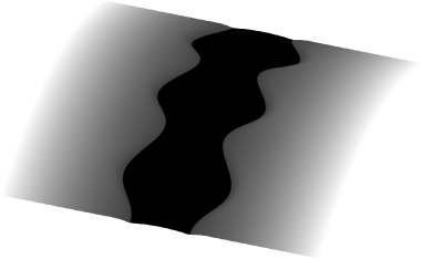
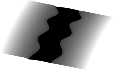
Figure 5: Two types of buckling modes: (a) Symmetric (varicose) and (b) antisymmetric (sinuous) perturbations.

The type of symmetry dictates the initial condition at the center of symmetry, $x=0$. A varicose perturbation, shown in figure 5a, is denoted by a superscript $(+)$ as it is symmetric with respect to the $x$ axis; for this type of symmetry, the conditions $u_{x}^{1W}(0)=u_{y}^{1W^{\prime}}(0)=0$ hold. A sinuous perturbation, shown in figure 5b, is denoted by a superscript $(-)$ as it is antisymmetric with respect to the $x$ axis; for this other type of symmetry, the conditions $u_{x}^{1W^{\prime}}(0)=u_{y}^{1W}(0)=0$ hold. We can thus define two independent initial state vectors in the wet region as follows: for the analysis of the varicose mode, $\underline{U}_{W}^{+,1}(0)=[0,1,0,0]$ and $\underline{U}_{W}^{+,2}(0)=[0,0,1,0]$. For the analysis of the sinuous mode, $\underline{U}_{W}^{-,1}(0)=[1,0,0,0]$ and $\underline{U}_{W}^{-,2}(0)=[0,0,0,1]$. A generic initial condition compatible with the symmetry is obtained by linear superposition, using two unknown amplitudes which we denote $i_{5}$ and $i_{6}$:

$$\underline{U}_{W}^{\pm}(0)=\sum_{j=1}^{2}i_{j+4}\,\underline{U}_{W}^{\pm,j}(0)\textrm{.}$$ (72)

Integrating equation (66a) across the wet region $\Omega_{F}$ using each of the various modes in equation (72) successively, we compute a shoot matrix for the wet region:

$$\underline{U}_{W}^{\pm}(a_{0}^{-})=\underline{\underline{\mathcal{S}}}_{W}^{\pm}(\nu,\sigma,k)\cdot\underline{I}_{W}\textrm{.}$$ (73)

There are in fact two such shoot matrices, one for each type of symmetry, and with size $4\times 2$ each.

4.5 Assembly

Let us define an assembled state vector at the boundary $x=a_{0}$ by collecting those relevant to the free and wet regions:

$$\underline{U}(a_{0})=[\underline{U}_{F}(a_{0}^{+}),\underline{U}_{W}^{\pm}(a_{0}^{-}),a_{1}]\textrm{.}$$ (74)

We have also appended the perturbation $a_{1}$ of the boundary shape, which will soon be needed.

We can similarly define an assembled shoot vector by

$$\underline{I}=[\underline{I}_{F},\underline{I}_{W},a_{1}]\textrm{.}$$ (75)

This $\underline{I}$ is the main unknown of our stability problem, and will be shown to satisfy an eigenvalue problem.

Then equations (71) and (73) can be rewritten in compact form as:

$$\underline{U}(a_{0})=\underline{\underline{\mathcal{S}}}_{WF}^{\pm}(\nu,\sigma,k)\cdot\underline{I}$$ (76)

where the global shoot matrix $\underline{\underline{\mathcal{S}}}_{WF}^{\pm}$ is formed by assembling into blocks the shoot matrices previously computed:

$$\underline{\underline{\mathcal{S}}}_{WF}^{\pm}(\nu,\sigma,k)=\begin{pmatrix}\underline{\underline{\mathcal{S}}}_{F}&0&0\\ 0&\underline{\underline{\mathcal{S}}}_{W}^{\pm}&0\\ 0&0&1\end{pmatrix}\textrm{.}$$ (77)

Its size is $13\times 7$.

4.6 Equilibrium of the moving boundary

At this point, we are ready to close the formulation of the stability problem by using the remaining continuity and jump conditions at the edge of the contact region. Upon linearization, the seven conditions (49) can be written in matrix notation as:

$$\underline{\underline{\mathcal{C}}}(\nu,\sigma,k)\cdot\underline{U}(a_{0})=\underline{0}\emph{.}$$ (78)

The matrix $\underline{\underline{\mathcal{C}}}$ is of size $7\times 7$. It collects the coefficients appearing in these linearized equations. The equations (49) hold on the mobile curve $x=g_{+}(x)$ which is perturbed according to equation (64). As a result, the linearized equations have terms proportional to the boundary perturbation $a_{1}$ times the gradients of the base solution, and these terms are used to fill the last column of $\underline{\underline{\mathcal{C}}}$. This allows the perturbation to the boundary to be treated without approximation.

Note that the inhomogeneous term $(-2\,\sigma)$ appearing in the right-hand side of the adhesion condition (49g) disappears upon linearization.

4.7 Linear stability formulated as an eigenproblem

By combining the equilibrium of the interface in equation (78) and the integration in the free and wet domain captured in equation (76), we can write the linear stability problem as an eigenvalue problem,

$$\big{[}\underline{\underline{\mathcal{C}}}(\nu,\sigma,k)\cdot\underline{\underline{\mathcal{S}}}_{WF}^{\pm}(\nu,\sigma,k)\big{]}\cdot\underline{I}=\underline{0}\textrm{.}$$ (79)

The existence of a linearly unstable mode requires

$$\det{\big{[}\underline{\underline{\mathcal{C}}}(\nu,\sigma,k)\cdot\underline{\underline{\mathcal{S}}}_{WF}^{\pm}(\nu,\sigma,k)\big{]}}=0\textrm{.}$$ (80)

This is an implicit equation for the wave number $k$ as a function of the adhesion parameter $\sigma$ and of Poisson’s ratio $\nu$. The corresponding eigenvector $\underline{I}$ allows the linearly unstable mode to be reconstructed.

4.8 Numerical results

We explained how the shoot matrix $\underline{\underline{\mathcal{S}}}_{WF}^{\pm}(\nu,\sigma,k)$ and the linearized equilibrium of the boundary $\underline{\underline{\mathcal{C}}}(\nu,\sigma,k)$ can be computed numerically for specific values of their arguments. For a given value of Poisson’s ratio $\nu$ and for each type of symmetry, we repeatedly computed the determinant for different values of $\sigma$ and $k$, and then plotted the implicit curve defined by equation (80) in the plane $(k,\sigma)$. The result is shown in figure 6a for a typical value of Poisson’s ratio, $\nu=0.4$.

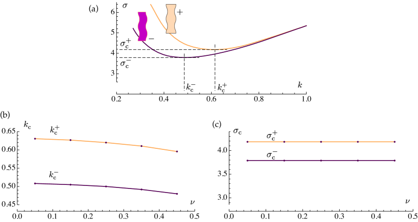
Figure 6: (a) Linear stability diagram for $\nu=0.4$. The most unstable symmetric and antisymmetric modes are defined by $\sigma_{c}^{\pm}$ and $k_{c}^{\pm}$ (b,c) Dependence of the critical wavevector $k_{c}^{\pm}$ and adhesion number $\sigma_{c}^{\pm}$ on Poisson’s ratio.

Numerical convergence with respect to the parameter $x_{m}$ required in the calculation of the shoot matrix $\underline{\underline{\mathcal{S}}}_{F}$ was attested by the fact that further increase of $x_{m}$ did not significantly affect the stability curves; typically, this required $x_{m}\approx 12$.

The most unstable wavenumber $k_{\mathrm{c}}^{\pm}$ and the critical adhesion $\sigma_{\mathrm{c}}^{\pm}$ correspond to the minimum of each of the curves in the plane $(k,\sigma)$. For each type of symmetry, the most unstable mode depends only on Poisson’s ratio, hence the notations $\sigma_{\mathrm{c}}^{\pm}(\nu)$ and $k_{\mathrm{c}}^{\pm}(\nu)$. The corresponding curves are plotted in figure 6b and c.

The stability analysis predicts that the most unstable mode is always the antisymmetric (sinuous) one. Indeed, the curve corresponding to this mode is always below the other curve in figure 6c. This is consistent with the experiments, where the varicose mode has never been observed.

It turns out that the dependence of both $\sigma_{\mathrm{c}^{\pm}}(\nu)$ and $k_{\mathrm{c}}^{\pm}(\nu)$ on Poisson’s ratio can be captured by simple formulas which match the numerical results perfectly, within numerical accuracy:

$$k_{\mathrm{c}}^{-}(\nu) \approx\frac{0.718}{x^{*}(\nu)} \qquad\sigma_{\mathrm{c}}^{-}(\nu) \approx 3.788\textrm{,}$$ (81a)

$$k_{\mathrm{c}}^{+}(\nu) \approx\frac{0.891}{x^{*}(\nu)} \qquad\sigma_{\mathrm{c}}^{+}(\nu) \approx 4.184\textrm{,}$$ (81b)

where $x^{*}(\nu)$ is the function defined in equation (57). We have no explanation to offer for the fact that $\sigma_{\mathrm{c}}^{\pm}$ is independent of $\nu$, and that $k_{\mathrm{c}}^{\pm}(\nu)$ depends on $\nu$ as $1/x^{*}(\nu)$. This probably points to the fact that a proper rescaling of the various quantities would allow the parameter $\nu$ to be removed from the linearized equations altogether. We have not been able, however, to identify such a rescaling.

The predictions relevant to the experiments, where we used a film with Poisson’s ratio $\nu=0.4$, are

$$\sigma_{\mathrm{c}}^{-}(0.4)=3.788,\qquad k_{\mathrm{c}}^{-}(0.4)=0.486,\qquad\ell_{\mathrm{c}}^{-}=\frac{2\,\pi}{k_{\mathrm{c}^{-}}(0.4)}=12.93\textrm{.}$$ (82)

Here $\ell_{\mathrm{c}}^{-}$ denotes the wavelength of the sinuous instability. These results are in qualitative agreement with the picture shown in figure 1: the straight contact region looses stability somewhere between $\sigma=1.37$ and $\sigma=4.01$, and the buckled pattern is indeed sinuous (antisymmetric). A detailed and systematic comparison to the experiments is presented in the following section, using a novel experimental setup that allows the adhesion number $\sigma$ to be varied continuously.

5 Comparison to experiments

In order to check the predictions of the linear stability analysis, we have developed a novel experimental setup that allows the adhesion parameter $\sigma$ to be continuously varied while the shape of the contact area is monitored. To do so, we replaced the rigid spheres used in previous work [18] by an inflatable latex membrane. The membrane was cut out in a latex sheet with Young’s modulus $E_{\mathrm{m}}=1.2~{}\mathrm{MPa}$ and thickness $h_{\mathrm{m}}=0.6~{}\mathrm{mm}$, and glued on top of vertical rigid cylinders with radius $\rho_{\mathrm{cyl}}=20,38,100,295~{}\mathrm{mm}$, see figure 7a.

Figure 7: (a,b) Experimental setup. A square latex sheet glued on top of a rigid cylinder is inflated by a pressure $\Delta p$ and deforms into a spherical cap. It is coated with ethanol and a thin film is applied onto it. (c,d) Experimental images of the adhering regions, as viewed from top: the darker strip corresponds to the contact zone. Decreasing the pressure $\Delta p$ increases the adhesion parameter $\sigma$, and induces a transition from straight to oscillatory edges.

Increasing the pressure by $\Delta p$ inside the cylindrical container allows the radius of the latex sheet to be varied continuously from $\rho=\infty$ when the membrane is flat, to $\rho=\rho_{\mathrm{cyl}}$ when it is half a sphere; the adhesion parameter $\sigma$ then varies according to equation (19). We checked that the shape of the membrane is almost spherical. The value of the radius of curvature $\rho(\Delta p)$ was measured from pictures taken from the side.

The spherical cap was then coated with ethanol, whose surface tension is $\gamma=22.4~{}\mathrm{mN}\,\mathrm{m}^{-1}$. Thin polypropylene films were applied on top of it, as shown in figure 7b. The films, produced by Innovia films, have a Young’s modulus $E=2.6\pm 0.2~{}\mathrm{GPa}$, a Poisson’s ratio $\nu=0.4$, and their thickness ranges from $h=15\,\mu\mathrm{m}$ to $90\,\mu\mathrm{m}$. Ethanol was chosen because it wets both latex and polypropylene, and because its surface tension is not very sensitive to impurities. Snapshots are simultaneously taken from top and from the side to monitor the shape of the pattern as a function of the radius of the spherical cap. The transition from band-like contact pattern to sinuous pattern was observed as a result of membrane deflation, see figure 7c,d.

The typical evolution of the edges profile as a function of the radius $\rho$ is shown in figure 8a.

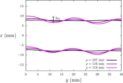
Figure 8: (a) Evolution of the edges as a function of the radius of the spherical cap $\rho$. All curves correspond to the same film, $h=50~{}\mu\mathrm{m}$. (b,c) Evolution of the rescaled amplitude $a_{1}$ of the edge profile as a function of the reduced adhesion number $\sigma$. Variations of $\sigma$ have been achieved by deflating the membrane. The experiment has been repeated three times using the same film with thickness $h=50~{}\mu\mathrm{m}$, and the symbols correspond to the different experiments. The value of the threshold is very reproducible, but the amplitude of buckling in the post-buckled regime is more scattered.

The edges remain straight until the sphere reaches a critical radius $\rho_{c}$ and then become undulatory; the amplitude of undulation increases as $\rho$ is further increased. The observed buckled patterns are always sinuous, as predicted by the stability analysis. By fitting the edges profile with a cosine function $a_{1}\cos{(kx+\phi)}$, we extracted the wavelength and the amplitude of the oscillations. Our measurements for a particular polypropylene film ($h=50~{}\mu\mathrm{m}$) are collected in figure 8b, which shows the dependence of the amplitude of oscillation on the sphere radius. The amplitude of the undulations goes to zero at the instability threshold, which is consistent with a supercritical bifurcation. When the experiment is repeated several times using the same film, the value of the bifurcation threshold is found to be quite reproducible. The scattering of the data for the buckling amplitude well above the threshold may attributed to variations in the volume of ethanol used, to friction between the film and the sphere, and to variations in the way that the film is initially laid out on the sphere.

Restoring the physical units, we rewrite the predictions of the analysis of linear stability in equation (82) as

$$\rho_{\mathrm{c}}(0.4)=3.788\,L_{ec},\qquad\ell_{\mathrm{c}}(0.4)=13.52\,\sqrt{h\,L_{ec}}\textrm{.}$$ (83)

We recall that $\rho_{\mathrm{c}}$ and $\ell_{\mathrm{c}}$ denote the radius of curvature of the sphere, and the wavelength of the pattern at threshold, respectively.

In figure 9 we compare these predictions to the experiments.

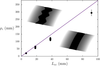
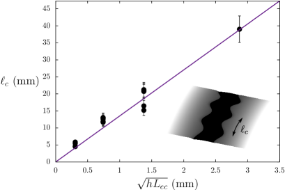
Figure 9: (a) Critical radius of sphere $\rho_{c}$ leading to undulations of the contact region, as a function of the elastocapillary length $L_{ec}$. Each data point corresponds to a specitif film thickness, and is obtained by detecting the threshold of instability in the experimental curve for $a_{1}(\rho)$, as in figure 7b. The various data points correspond to thicknesses $h$ ranging from $15~{}\mathrm{\mu m}$ to $90~{}\mathrm{\mu m}$. Note the collapse of these points onto a single curve. (b) Wavelength of the oscillations $\ell_{c}=2\pi/k_{c}$ at threshold ($\rho=\rho_{c}$). In (a) and (b), the solid lines show to the prediction of the analysis of linear stability in equation (83) for $\nu=0.4$, with no adjustable parameter.

The elastocapillary length $L_{ec}$ is computed from the experimental parameters using equation (20). The wavelength of the pattern agrees very well with the prediction of the analysis of linear stability; there is no adjustable parameter. The agreement concerning the instability threshold is not as good but satisfactory; as apparent in Figure 7d, the actual threshold is lower by about $15\%$ than that predicted by theory. This can probably be attributed to imperfections in the planarity of the film and in the way that it is layout onto the substrate, as well as to the finite size of the meniscus.

6 Conclusion

We have investigated the adhesion of a thin film on a spherical substrate. The Donnell theory of nearly cylindrical shells has been used, taking into account the energy of adhesion with the sphere. We have derived the boundary conditions holding at the edge of the moving boundary between the wet and free regions. A family of nonlinear solutions describing the unbuckled configuration of the film has been constructed. These solutions, which have cylindrical symmetry, are indexed by a dimensionless adhesion number $\sigma=\rho/L_{ec}$, that compares the radius of curvature of the sphere $\rho$ to the elastocapillary length $L_{ec}$. As the adhesion number $\sigma$ increases, a compressive stress builds up along the edge of the contact zone and makes the film buckle. We have carried out a linear stability analysis of the unbuckled solution, taking into account the motion of the moving boundary between the wet and free regions, and found of a critical value of the adhesion number $\sigma$ above which the contact region becomes sinous. The symmetry of the unstable mode, as well as the instability threshold and the wavelength found by the theory are in good agreement with the experiments.

In our system, buckling is driven by the geometric frustration due to the mismatch between the Gauss curvature of the substrate and that of the planar film; a related type of buckling driven by geometric frustration has been investigated in plates undergoing swelling [29], and in annular origami models having a curved crease [30]. Our paper provides a detailed analysis of the initial buckling of our system. Far above the buckling threshold, the buckling patterns evolve into a branched network of bands whose edges are made up by a series of cusps. These singularities seem to be connected with the existence of developable cones and sharp ridges in the free parts of the film, and are not yet understood in detail.

Appendix A A justification of the Donnell equations by formal asymptotic expansion

The Donnell equations for shells are justified by a formal expansion with respect to a small parameter $\eta$ proportional to the square-root of the aspect-ratio of the shell. Assuming that the transverse displacement is of order $\eta^{2}$, we derive these equations from the general non-linear equations for elastic shells under finite displacement. The present derivation is mainly given for pedagogical purposes as a rigorous proof is available in [31]. Note that formal expansions have also been used to justify plate equations in [32].

A.1 Transformation

Let us first define the cylindrical basis vectors

$$\underline{e}_{1}(\theta)=\left(\begin{array}[]{c}0\\ \cos\theta\\ \sin\theta\end{array}\right),\qquad\underline{e}_{2}(\theta)=\left(\begin{array}[]{c}0\\ -\sin\theta\\ \cos\theta\end{array}\right)\textrm{.}$$ (84)

This basis is such that $\underline{e}_{1}^{\prime}(\theta)=\underline{e}_{2}(\theta)$, $\underline{e}_{2}^{\prime}(\theta)=-\underline{e}_{1}(\theta)$, and $\underline{e}_{1}(\theta)\times\underline{e}_{2}(\theta)=\underline{e}_{X}$: the polar axis is the axis $X$ of the shell in reference configuration.

In the reference configuration, the shell is rolled into a cylinder of radius $\rho$. We use Lagrangian coordinates $(x,y)$. The position in reference configuration is denoted $\underline{x}$, as shown in figure 2a,

$$\underline{x}(x,y)=\rho\,\underline{e}_{1}(\theta)+x\,\underline{e}_{x},\quad\textrm{where }\theta=\frac{y}{\rho}\textrm{.}$$

Note that the metric associated with the set of coordinates $(x,y)$ is the unit tensor, $\underline{\underline{\nabla}}\underline{x}^{T}\cdot\underline{\underline{\nabla}}\underline{x}=\underline{\underline{1}}$.

The deformed configuration $\underline{\tilde{x}}$ is defined in terms of the displacement $(u_{x}(x,y),u_{y}(x,y),w(x,y))$ in cylindrical coordinates by equation (1), and is also sketched in figure 2b.

The strain in the shell is measured using a membrane strain tensor $\underline{\underline{e}}$ and a curvature strain tensor $\underline{\underline{b}}$. The nonlinear membrane strain $\underline{\underline{e}}$ is a $2\times 2$ symmetric tensor defined by the classical formula:

$$\underline{\underline{F}}=\underline{\underline{\nabla}}\underline{\tilde{x}},\quad\underline{\underline{C}}=\underline{\underline{F}}^{T}\cdot\underline{\underline{F}},\quad\underline{\underline{e}}=\frac{1}{2}\,(\underline{\underline{C}}-\underline{\underline{1}})\textrm{,}$$ (85)

where the gradient is taken with respect to the Lagrangian coordinates $(x,y)$. The curvature strain tensor is defined by

$$b_{\alpha\beta}=\underline{\tilde{x}}_{,\alpha\beta}(x,y)\cdot\underline{N}(x,y)$$ (86a)

where the normal to the shell is defined by

$$\underline{N}(x,y)=-\underline{\tilde{x}}_{,x}(x,y)\times\underline{\tilde{x}}_{,y}(x,y)\textrm{.}$$ (86b)

The minus sign in the definition of the normal in equation (86b) makes the normal $\underline{N}$ oriented in same direction as the radial vector $\underline{e}_{1}(\theta)$ of the cylindrical basis. Note that the normal is not a unit normal if the current configuration is not developable, $e_{\alpha\beta}\neq 0$. Since we consider deformations that are almost inextensible, our definition (86a) of the bending strain is very close to the geometrically exact definition of the curvature that makes use of a unit normal vector, and this introduces a higher-order correction in the thin-shell limit.

By inserting equation (1) into equation (85), one could rederive the fully non-linear expression of the 3 independent components $e_{\alpha\beta}$ in terms of the displacement functions $(u_{x},u_{y},w)$, relevant to the general theory of shells under finite displacements. Similarly, by inserting into equation (86), one could derive a fully non-linear expression for the curvature strains $b_{\alpha\beta}$.

A.2 Formal expansion of the membrane and curvature strains

The Donnell equations are derived from the above set of equations under the assumption of a moderate displacement. We consider a formal expansion of the above equations with respect to a small parameter $\eta$. The definition of $\eta$ given in equation (9) will be justified. For the moment, it is sufficient to assume $\eta\ll 1$. We assume that the transverse displacement $w$ scales like $\rho\,\eta^{2}$, that the in-plane displacement scales like $\rho\,\eta^{3}$, and that the typical scale for the tangent coordinates $x$ and $y$ is $\rho\,\eta$. The dimensionless displacement $\overline{u}_{\alpha}(\overline{x},\overline{y})$ and $\overline{w}(\overline{x},\overline{y})$ are defined in equation (11) in terms of the rescaled coordinates $\overline{x}=x/(\rho\,\eta)$ and $\overline{y}=y/(\rho\,\eta)$.

The previous scalings can be justified as follows. Our starting assumption is that the deflection $w$ is small, and scales as $\rho\,\eta^{2}$. From this, as $w\sim x^{2}/\rho$ along the curved shell, it appears that the natural scale for the tangent coordinates is $\rho\,\eta$. Balancing the linear and non-linear terms in the membrane strain, we have $u_{\alpha,x}\sim w_{,x}^{2}$ and so the scale for the tangential displacement is $\rho\,\eta^{3}$.

Expanding the membrane strain $\underline{\underline{e}}$ introduced in equation (85) with respect to $\eta$, one computes

$$e_{\alpha\beta}(x,y)=\eta^{2}\,\overline{e}_{\alpha\beta}(\overline{x},\overline{y})+\mathcal{O}(\eta^{4})\textrm{,}\\$$ (87)

where the dominant contribution is given by

$$\overline{e}_{\alpha\beta}(\overline{x},\overline{y})=\left(\frac{\overline{u}_{\alpha,\beta}(\overline{x},\overline{y})+\overline{u}_{\beta,\alpha}(\overline{x},\overline{y})}{2}+\delta_{\alpha y}\,\delta_{\beta y}\,\overline{w}(\overline{x},\overline{y})\right)+\frac{1}{2}\,\overline{w}_{,\alpha}(\overline{x},\overline{y})\,\overline{w}_{,\beta}(\overline{x},\overline{y})\textrm{.}$$ (88)

This result was stated in equation (14a) but with the bars omitted. In the right-hand side, the derivatives are taken with respect to the rescaled variables, for instance $\overline{u}_{\alpha,\beta}=\partial\overline{u}_{x}/\partial\overline{y}$ when $\alpha=x$ and $\beta=y$.

A similar expansion of the curvature strain defined in equation (86) yields

$$b_{\alpha\beta}(x,y)=\frac{\eta^{0}}{\rho}\,\overline{b}_{\alpha\beta}(\overline{x},\overline{y})+\mathcal{O}(\eta^{2})$$ (89)

where the dominant contribution reads

$$\overline{b}_{\alpha\beta}(\overline{x},\overline{y})=-\overline{w}_{,\alpha\beta}(\overline{x},\overline{y})\textrm{.}$$ (90)

The minus sign in the right-hand side comes from that introduced in the definition of the normal $\underline{N}$.

A.3 Rescaled constitutive equations, elastic energy

For an isotropic, Hookean (linearly elastic) material, the constitutive laws read, in physical units:

$$n_{\alpha\beta} =C\,((1-\nu)\,e_{\alpha\beta}+\nu\,(\operatorname{tr}\underline{\underline{e}})\,\delta_{\alpha\beta})$$ (91a)

$$m_{\alpha\beta} =D\,((1-\nu)\,b_{\alpha\beta}+\nu\,(\operatorname{tr}\underline{\underline{b}})\,\delta_{\alpha\beta})$$ (91b)

where $C=Eh/(1-\nu^{2})$ and $D=Eh^{3}/[12(1-\nu^{2})]$ are the stretching and bending moduli, respectively. It is convenient to define the slenderness parameter $\eta$ by

$$\eta=\left(\frac{D}{C\,\rho^{2}}\right)^{1/4}=\left(\frac{1}{\sqrt{12}}\,\frac{h}{\rho}\right)^{1/2}\textrm{,}$$ (92)

as we did earlier in equation (9). Indeed, this convention makes both the stretching and bending moduli $C$ and $D$ effectively equal to one in rescaled units.

The elastic energy of the shell reads

$$E_{\mathrm{shell}}=\frac{1}{2}\,\iint(n_{\alpha\beta}\,e_{\alpha\beta}+m_{\alpha\beta}\,b_{\alpha\beta})\,\mathrm{d}x\,\mathrm{d}y$$ (93)

and can be rescaled as

$$E_{\mathrm{shell}}=\rho^{2}\,C\,\eta^{4}\,\overline{E}_{\mathrm{shell}}\textrm{,}$$ (94)

where

$$\overline{E}_{\mathrm{shell}}=\frac{1}{2}\,\iint(\overline{n}_{\alpha\beta}\,\overline{e}_{\alpha\beta}+\overline{m}_{\alpha\beta}\,\overline{b}_{\alpha\beta})\,\mathrm{d}\overline{x}\,\mathrm{d}\overline{y}\textrm{.}$$ (95)

The dimensionless stress can be computed by the dimensionless version of the constitutive law, see equation (16).

As shown in section 2.6, Donnell equations then follow by variational principles from the shell energy (95) combined with the definitions (88) and (90) of the membrane and curvature strains, and with the rescaled constitutive laws (16). These definitions (88) and (90) are often presented as approximation. We have just shown that they follow from scaling assumptions and are asymptotically exact for small displacement.

Appendix B Two-dimensional Weierstrass-Erdmann corner conditions

With the aim to derive the jump conditions at the interface between the adhering part and the free part of the shell, we recall the Weierstrass-Erdmann corner conditions in a generic two-dimensional setting. We refer to [33] for a detailed presentation. We consider a two-dimensional domain $\Omega$ that is split in two regions $\Omega_{1}$ and $\Omega_{2}$ meeting along a boundary curve $G=\Omega_{1}\cap\Omega_{2}$, as depicted in figure 10.

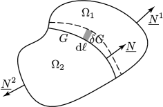
Figure 10: Equilibrium of a mobile interface $G$ between two domains $\Omega^{1}$ and $\Omega^{2}$.

The unknowns are the functions $\xi_{\alpha}(x,y)$ where $\alpha$ is an index, such as the component of the displacement in the case of an adhering shell. Each region $\Omega_{i}$, $i=1,2$ is associated with a specific Lagrangian (also called energy functional),

$$E_{i}(\xi_{\alpha},G)=\int_{\Omega_{i}(G)}\mathcal{L}^{i}(\xi_{\alpha},\xi_{\alpha,\beta})\,\mathrm{d}x\,\mathrm{d}y\textrm{.}$$ (96)

The boundary may evolve and we use the boundary curve $G$ as an unknown: the domains $\Omega_{i}$ are reconstructed in terms of the curve $G$, hence the notation $\Omega_{i}(G)$.

We are interested in the conditions that make the total energy $E=E_{1}+E_{2}$ minimum, and in particular in the conditions associated with the motion of the interface $G$. The variation $\delta E$ of the total energy is made up of a term arising from the variation of the functions $\xi_{\alpha}(x,y)$ inside each domain, and from a term associated with the motion of the free boundary,

$$\delta E=\sum_{i=1}^{2}\int_{\Omega_{i}(G)}\left(\frac{\partial\mathcal{L}^{i}}{\partial\xi_{\alpha}}\,\delta\xi_{\alpha}+\frac{\partial\mathcal{L}^{i}}{\partial\xi_{\alpha,\beta}}\,\delta\xi_{\alpha,\beta}\right)+\int_{G}(\mathcal{L}^{2}-\mathcal{L}^{1})\;\delta G\,\mathrm{d}\ell\textrm{.}$$ (97)

Here the partial derivatives denote functional derivative, $\mathrm{d}\ell$ is the element of length along the boundary $G$, and $\delta G\,\mathrm{d}\ell$ is the signed area swept by the free boundary, counted positively when the region $\Omega_{2}$ grows while the region $\Omega_{1}$ shrinks, as shown in figure 10.

We consider the contribution $\delta E_{G}$ to $\delta E$ that collects all terms written as integrals along the boundary curve $G$. These terms yield the jump conditions associated with the equilibrium of the boundary, while the other terms contribute to the Euler-Lagrange conditions of equilibrium inside each subdomain. This $\delta E_{G}$ is made up of the last term in equation (97), and of a term coming from the integration by part of the term proportional to $\delta\xi_{\alpha,\beta}$,

$$\delta E_{G}=\int_{G}\left([\![\mathcal{L}^{i}]\!]\,\delta G+[\![\frac{\partial\mathcal{L}^{i}}{\partial\xi_{\alpha,\beta}}\,\delta\xi_{\alpha}]\!]\,N_{\beta}\right)\,\mathrm{d}\ell\textrm{.}$$ (98)

Here the double bracket denotes the jump, $[\![f^{i}]\!]=f^{2}-f^{1}$ and $\underline{N}=(N_{x},N_{y})$ is the vector normal to the boundary $G$, directed towards region 1 as in the figure. Along the common boundary $G$, this $\underline{N}$ is equal to the outward normal $\underline{N}^{2}$ with respect to the domain $\Omega_{2}$, and is opposite to the outward normal $\underline{N}^{1}$ to domain $\Omega_{1}$.

We shall assume that the unknown $\xi_{\alpha}$ is prescribed to be continuous across the boundary, as happens with the components of the displacement and with the slope $q_{\alpha}=w_{,\alpha}$ of an elastic shell,

$$[\![\xi_{\alpha}]\!]=0\textrm{.}$$ (99)

This continuity relation can be differentiated in a frame moving along with the boundary. This yields, for an arbitrary perturbation of the boundary and of the function,

$$[\![\delta\xi_{\alpha}]\!]+[\![\xi_{\alpha,\beta}]\!]\,N_{\beta}\,\delta G=0$$ (100)

First, consider perturbations leaving the boundary unchanged, $\delta G=0$. Then equation (100) shows that $\delta\xi_{\alpha}$ is continuous across the boundary as $[\![\delta\xi_{\alpha}]\!]=0$. In the expression for $\delta E_{G}$ given in equation (98), the first term cancels when the free boundary is at rest, and $\delta\xi_{\alpha}$ can be factored out of the jump operator, yielding the condition

$$[\![\frac{\partial\mathcal{L}^{i}}{\partial\xi_{\alpha,\beta}}]\!]\,N_{\beta}\,\delta\xi_{\alpha}=0\textrm{.}$$ (101)

In the particular case of a function $\xi_{\gamma}$ whose values are prescribed in the domain $\Omega_{1}$, we have $\delta\xi_{\gamma}^{1}=0$. The continuity condition (101) then yields $\delta\xi_{\gamma}^{2}+[\![\xi_{\gamma,\beta^{\prime}}]\!]\,N_{\beta^{\prime}}\,\delta G=0$. Cancelling the variation in equation (98) then yields

$$\textrm{if $\delta\xi_{\gamma}$ is prescribed on $\Omega_{1}$, then }\mathcal{L}^{2}-\mathcal{L}^{1}-\frac{\partial\mathcal{L}^{2}}{\partial\xi_{\gamma,\beta}}\,[\![\xi_{\gamma,\beta^{\prime}}]\!]\,N_{\beta^{\prime}}\,N_{\beta}=0\textrm{.}$$ (102)

References

- [1] S. Timoshenko, S. Woinowski-Krieger, Theory of plates and shells, McGraw-Hill, 1959.
- [2] S. Timoshenko, J. Gere, Theory of elastic stability, Dover, 2009.
- [3] J. Singer, J. Arbocz, T. Weller, Buckling Experiments, Experimental Methods in Buckling of Thin-Walled Structures, Volume 1, Basic Concepts, Columns, Beams and Plates, Wiley, 1997.
- [4] A. Geim, K. Novoselov, The rise of graphene, Nature Mater. 6 (2007) 183–191.
- [5] J. Shim, C. Perdigou, E. Chen, K. Bertoldi, P. Reis, Buckling-induced encapsulation of structured elastic shells under pressure, Proc. Natl. Acad. Sci. USA doi:10.1073/pnas.010123497.
- [6] B. Davidovitch, R. Schroll, D. Vella, M. Adda-Bedia, E. Cerda, Prototypical model for tensional wrinkling in thin sheets, Proc. Natl. Acad. Sci. USA 108 (2011) 18227–18232.
- [7] E. Hohlfeld, L. Mahadevan, Unfolding the sulcus, Phys. Rev. Lett. 106 (2011) 105702.
- [8] Y. Cao, J. W. Hutchinson, From wrinkles to creases in elastomers: the instability and imperfection-sensitivity of wrinkling, Proc. R. Soc. A 468 (2137) (2011) 94–115.
- [9] X. Chen, J. W. Hutchinson, Herringbone buckling patterns of compressed thin films on compliant substrates, J. Appl. Mech. 71 (5) (2004) 597–603.
- [10] B. Audoly, A. Boudaoud, Buckling of a thin film bound to a compliant substrate (part 3). Herringbone solutions at large buckling parameter, J. Mech. Phys. Solids 56 (7) (2008) 2444–2458.
- [11] S. Cai, D. Breid, A. J. Crosby, Z. Suo, J. W. Hutchinson, Periodic patterns and energy states of buckled films on compliant substrates, J. Mech. Phys. Solids 59 (5) (2011) 1094–1114.
- [12] B. Li, Y.-P. Cao, X.-Q. Feng, H. Gao, Mechanics of morphological instabilities and surface wrinkling in soft materials: a review, Soft Matter doi:10.1039/C2SM00011C.
- [13] G. Gioia, M. Ortiz, Delamination of compressed thin films, Adv. Appl. Mech. 33 (1997) 119–192.
- [14] D. Vella, J. Bico, A. Boudaoud, B. Roman, P. Reis, The macroscopic delamination of thin films from elastic substrates, Proc. Natl. Acad. Sci. USA 106 (2009) 10901.
- [15] J. Hutchinson, Z. Suo, Mixed mode cracking in layered materials, Adv. Appl. Mech. 29 (1992) 63–191.
- [16] B. Audoly, Mode-dependent toughness and the delamination of compressed thin films, J. Mech. Phys. Solids 48 (11) (2000) 2315–2332.
- [17] J. Bico, B. Roman, L. Moulin, A. Boudaoud, Elastocapillary coalescence in wet hair, Nature 432 (2004) 690.
- [18] J. Hure, B. Roman, J. Bico, Wrapping an adhesive sphere with a elastic sheet, Phys. Rev. Lett. 106 (2011) 174301.
- [19] K. Tamura, S. Komura, T. Kato, Adhesion induced buckling of spherical shells, J. Phys.: Condens. Matter 16 (2004) L421–L428.
- [20] S. Komura, K. Tamura, T. Kato, Buckling of spherical shells adhering onto a rigid substrate, Eur. Phys. J. E 18 (2005) 343–358.
- [21] R. Springman, J. Bassani, Snap transitions in adhesion, J. Mech. Phys. Solids 56 (2008) 2358–2380.
- [22] D. Struik, Lectures on Classical Differential Geometry, Dover, 1988.
- [23] M. Amabili, Nonlinear vibrations and stability of shells and plates, Cambridge University Press, 2008.
- [24] B. Roman, J. Bico, Elasto-capillarity: deforming an elastic structure with a liquid droplet, J. Phys.: Condens. Matter 22 (2010) 493101.
- [25] E. Mansfield, The bending and stretching of plates, Cambridge University Press, 1989.
- [26] U. Seifert, Adhesion of vesicles in two dimensions, Phys. Rev. A 43 (1991) 6803–6814.
- [27] C. Majidi, G. Adams, A simplified formulation of adhesion problems with elastic plates, Proc. Roy. Soc. A 465 (2009) 2217–2230.
- [28] C. Majidi, G. Adams, Adhesion and delamination boundary conditions for elastic plates with arbitrary contact shape, Mechanics Research Communications 37 (2010) 214–218.
- [29] Y. Klein, E. Efrati, E. Sharon, Shaping of Elastic Sheets by Prescription of Non-Euclidean Metrics, Science 315 (5815) (2007) 1116–1120.
- [30] M. A. Dias, L. H. Dudte, L. Mahadevan, C. D. Santangelo, Geometric mechanics of curved crease origami, submitted to Physical Review Letters (2012).
- [31] I. Figueiredo, A justification of the donnell-mushtari-vlasov model by the asymptotic expansion, Asymptotic analysis 4 (1991) 257–269.
- [32] P. Ciarlet, A justification of the von kàrmàn equations, Arch. Ration. Mech. An. 73 (1980) 349–389.
- [33] J. Troutman, Variational calculus and optimal control, Springer, 1996.