Modelling fixation locations using spatial point processes

Abstract

Whenever eye movements are measured, a central part of the analysis has to do with where subjects fixate, and why they fixated where they fixated. To a first approximation, a set of fixations can be viewed as a set of points in space: this implies that fixations are spatial data and that the analysis of fixation locations can be beneficially thought of as a spatial statistics problem. We argue that thinking of fixation locations as arising from point processes is a very fruitful framework for eye movement data, helping turn qualitative questions into quantitative ones.

We provide a tutorial introduction to some of the main ideas of the field of spatial statistics, focusing especially on spatial Poisson processes. We show how point processes help relate image properties to fixation locations. In particular we show how point processes naturally express the idea that image features’ predictability for fixations may vary from one image to another. We review other methods of analysis used in the literature, show how they relate to point process theory, and argue that thinking in terms of point processes substantially extends the range of analyses that can be performed and clarify their interpretation.

Eye movement recordings are some of the most complex data available to behavioural scientists. At the most basic level they are long sequences of measured eye positions, a very high dimensional signal containing saccades, fixations, micro-saccades, drift, and their myriad variations (Ciuffreda and Tannen,, 1995). There are already many methods that process the raw data and turn it into a more manageable format, checking for calibration, distinguishing saccades from other eye movements (e.g., Engbert and Mergenthaler,, 2006; Mergenthaler and Engbert,, 2010). Our focus is rather on fixation locations.

In the kind of experiment that will serve as an example throughout the paper, subjects were shown a number of pictures on a computer screen, under no particular instructions. The resulting data are a number of points in space, representing what people looked at in the picture—the fixation locations. The fact that fixations tend to cluster shows that people favour certain locations and do not simply explore at random. Thus one natural question to ask is why are certain locations preferred?

We argue that a very fruitful approach to the problem is to be found in the methods of spatial statistics (Diggle,, 2002; Illian et al.,, 2008). A sizeable part of spatial statistics is concerned with how things are distributed in space, and fixations are “things” distributed in space. We will introduce the concepts of point processes and latent fields, and explain how these can be applied to fixations. We will show how this lets us put the important (and much researched) issue of low-level saliency on firmer statistical ground. We will begin with simple models and gradually build up to more sophisticated models that attempt to separate the various factors that influence the location of fixations and deal with non-stationarities.

Using the point process framework, we replicate results obtained previously with other methods, but also show how the basic tools of point process models can be used as building blocks for a variety of data analyses. They also help shed new light on old tools, and we will argue that classical methods based on analysing the contents of image patches around fixated locations make the most sense when seen in the context of point process models.

1 Analysing eye movement data

1.1 Eye movements

While looking at a static scene our eyes perform a sequence of rapid jerk-like movements (saccades) interrupted by moments of relative stability (fixations). One reason for this fixation-saccade strategy arises from the inhomogeneity of the visual field (Land and Tatler,, 2009). Visual acuity is highest at the center of gaze, i.e. the fovea (within 1° eccentricity), and declines towards the periphery as a function of eccentricity. Thus saccades are needed to move the fovea to selected parts of an image for high resolution analysis. About 3–4 saccades are generated each second. An average saccade moves the eyes 4–5° during scene perception and, depending on the amplitude, lasts between 20–50 ms. Due to saccadic suppression (and the the high velocity of saccades) vision is hampered during saccades (Matin,, 1974) and information uptake is restricted to the time in between, i.e. the fixations. During a fixation gaze is on average held stationary for 250–300 ms but individual fixation durations are highly variable and range from less than a hundred milliseconds to more than a second. For recent reviews on eye movements and eye movements during scene perception see Rayner, (2009) and Henderson, (2011), respectively.

During scene perception fixations cluster on “informative” parts of an image whereas other parts only receive few or no fixations. This behavior has been observed between and within observers and has been associated with several factors. Due to the close coupling of stimulus features and attention (Wolfe and Horowitz,, 2004) as well as eye movements and attention (Deubel and Schneider,, 1996), local image features like contrast, edges, and color are assumed to guide eye movements. In their influential model of visual saliency, Itti and Koch, (2001) combine several of these factors to predict fixation locations. However, rather simple calculations like edge detectors (Tatler and Vincent,, 2009) or center-surround patterns combined with contrast-gain control (Kienzle et al.,, 2009) seem to predict eye movements similarly well. The saliency approach has generated a lot of interest in research on the prediction of fixation locations and has led to the development of a broad variety of different models. A recent summary can be found in Borji and Itti, (2013).

Besides of local image features, fixations seem to be guided by faces, persons, and objects (Cerf et al.,, 2008; Judd et al.,, 2009). Recently it has been argued that objects may be, on average, more salient than scene background (Einhäuser et al.,, 2008; Nuthmann and Henderson,, 2010) suggesting that saccades might primarily target objects and that the relation between objects, visual saliency and salient local image features is just correlative in nature. The inspection behavior of our eyes is further modulated by specific knowledge about a scene acquired during the last fixations or more general knowledge acquired on longer time scales (Henderson and Ferreira,, 2004). Similarly, the same image viewed under differing instructions changes the distribution of fixation locations considerably (Yarbus,, 1967). To account for top-down modulations of fixation locations at a computational level, Torralba et al., (2006) weighted a saliency map with a-priori knowledge about a scene. Finally, the spatial distribution of fixations is affected by factors independent of specific images. Tatler, (2007), for example, reported a strong bias towards central parts of an image. In conventional photographs the effect may largely be caused by the tendency of photographers to place interesting objects in the image center but, importantly, the center bias remains in less structured images.

Eye movements during scene perception have been a vibrant research topic over the past years and the preceding paragraphs provide only a brief overview of the diverse factors that contribute to the selection of fixation locations. We illustrate the logic of spatial point processes by using two of these factors in the upcoming sections: local image properties—visual saliency—and the center bias. The concept of point processes can easily be extended to more factors and helps to assess the impact of various factors on eye movement control.

1.2 Relating fixation locations to image properties

There is already a rather large literature relating local image properties to fixation locations, and it has given rise to many different methods for analysing fixation locations. Some analyses are mostly descriptive, and compare image content at fixated and non-fixated locations. Others take a stronger modelling stance, and are built around the notion of a saliency map combining a range of interesting image features. Given a saliency map, one must somehow relate it to the data, and various methods have been used to check whether a given saliency map has something useful to say about eye movements. In this section we review the more popular of the methods in use. As we explain below, in Section 5.5 , the point process framework outlined here helps to unify and make sense of the great variety of methods in the field.

Reinagel and Zador, (1999) had observers view a set of natural images for a few seconds while their eye movements were monitored. They selected image patches around gaze points, and compared their content to that of control patches taken at random from the images. Patches extracted around the center of gaze had higher contrast and were less smooth than control patches. Reinagel and Zador’s work set a blueprint for many follow-up studies, such as Krieger et al., (2000) and Parkhurst and Niebur, (2003), although they departed from the original by focusing on fixated vs non-fixated patches. Fixated points are presumably the points of higher interest to the observer, and to go from one to the next the eye may travel through duller landscapes. Nonetheless the basic analysis pattern remained: one compares the contents of selected patches to that of patches drawn from random control locations.

Since the contents of the patches (e.g. their contrast) will differ both within-categories and across, what one typically has is a distribution of contrast values in fixated and control patches. The question is whether these distributions differ, and asking whether the distributions differ is mathematically equivalent to asking whether one can guess, based on the contrast of a patch, whether the patch comes from the fixated or the non-fixated set. We call this problem patch classification, and we show in Section 5.5.1 that it has close ties to point process modelling—indeed, certain forms of patch classification can be seen as approximations to point process modelling.

The fact that fixated patches have distinctive local statistics could suggest that it is exactly these distinctive local statistics that attract gaze to a certain area. Certain models adopt this viewpoint and assume that the visual system computes a bottom-up saliency map based on local image features. The bottom-up saliency map is used by the visual system (along with top-down influences) to direct the eyes (Koch and Ullman,, 1985). Several models of bottom-up saliency have been proposed (for a complete list see Borji and Itti,, 2013), based either on the architecture of the visual cortex (Itti and Koch,, 2001) or on computational considerations (e.g., Kanan et al.,, 2009), but their essential feature for our purposes is that they take an image as input and yield as output a saliency map. The computational mechanism that produces the saliency map should ideally work out from the local statistics of the image which areas are more visually conspicuous and give them higher saliency scores. The model takes its validity from the correlation between the saliency maps it produces and actual eye movements.

How one goes from a saliency map to a set of eye movements is not obvious, and Wilming et al., (2011) have found in their extensive review of the literature as many as 8 different performance measures. One solution is to look at area counts (Torralba et al.,, 2006): if we pick the 20% most salient pixels in an image, they will define an area that takes up 20% of the picture. If much more than 20% of the recorded fixations are in this area, it is reasonable to say that the saliency model gives us useful information, because by chance we’d expect this proportion to be around 20%.

A seemingly completely different solution is given by the very popular AUC measure (Tatler et al.,, 2005), which uses the patch classification viewpoint: fixated patches should have higher salience than control patches. The situation is analoguous to a signal detection paradigm: correctly classifying a patch as fixated is a Hit, incorrectly classifying a patch as fixated is a False Alarm, etc. A good saliency map should give both a high Hit Rate and a low rate of False Alarms, and therefore performance can be quantified by the area under the ROC curve (AUC): the higher the AUC, the better the model.

One contribution of the point process framework is that we can prove these two measures are actually tightly related, even though they are rather different in origin (Section 5.5.2). There are many other ways to relate stimulus properties to fixation locations, based for example on scanpaths (Henderson et al.,, 2007), on the number of fixations before entering a region of interest (Underwood et al.,, 2006), on the distance between fixations and landmarks (Mannan et al.,, 1996), etc. We cannot attempt here a complete unification of all measures, but we hope to show that our proposed spatial point process framework is general enough that such unification is at least theoretically possible. In the next section we introduce the main ideas behind spatial point-process models.

2 Point processes

We begin with a general overview on the art and science of generating random sets of points in space. It is important to emphasise at this stage that the models we will describe are entirely statistical in nature and not mechanistic: they do not assume anything about how saccadic eye movements are generated by the brain (Sparks,, 2002). In this sense they are more akin to linear regression models than, e.g., biologically-inspired models of overt attention during reading or visual search (Engbert et al.,, 2005; Zelinsky,, 2008). The goal of our modelling is to provide statistically sound and useful summaries and visualizations of data, rather than come up with a full story of how the brain goes about choosing where to allocate the next saccade. What we lose in depth, we gain in generality, however: the concepts that are highlighted here are applicable to the vast majority of experiments in which fixations locations are of interest.

2.1 Definition and examples

In statistics, point patterns in space are usually described in terms of point processes, which represent realisations from probability distributions over sets of points. Just like linear regression models, point processes have a deterministic and a stochastic component. In linear models, the deterministic component describes the average value of the dependent variable as a function of the independent ones, and the stochastic component captures the fact that the model cannot predict perfectly the value of the independent variable, for example because of measurement noise. In the same way, point processes will have a latent intensity function, which describes the expected number of points that will be found in a certain area, and a stochastic part which captures prediction error and/or intrinsic variability.

We focus on a certain class of point process models known as inhomogeneous Poisson processes. Some specific examples of inhomogeneous Poisson processes should be familiar to most readers. These are temporal rather than spatial, which means they generate random point sets in time rather than in space, but equivalent concepts apply in both cases.

In neuroscience, Poisson processes are often used to characterize neuronal spike trains (see e.g., Dayan and Abbott,, 2001). The assumption is that the number of spikes produced by a neuron in a given time interval follows a Poisson distribution: for example, repeated presentation of the same visual stimulus will produce a variable number of spikes, but the variability will be well captured by a Poisson distribution. Different stimuli will produce different average spike rates, but spike rate will also vary over time during the course of a presentation, for example rising fast at stimulation onset and then decaying. A useful description, summarized in Figure 1, is in terms of a latent intensity function $\lambda(t)$ governing the expected number of spikes observed in a certain time window. Formally, $\int_{\tau}^{\tau+\delta}\lambda\left(t\right)\mbox{d}t$ gives the expected number of spikes between times $\tau$ and $\tau+\delta$. If we note $\mathbf{t}=t_{1},t_{2},\ldots,t_{k}$ the times at which spikes occurred on a given trial, then $\mathbf{t}$ follows a inhomogeneous Poisson Process (from now on IPP) distribution if, for all intervals $\left(\tau,\tau+\delta\right)$, the number of spikes occurring in the interval follows a Poisson distribution (with mean given by the integral of $\lambda\left(t\right)$ over the interval).

The temporal IPP therefore gives us a distribution over sets of points in time (in Figure 1, over the interval $[0,1]$). Extending to the spatial case is straightforward: we simply define a new intensity function $\lambda(x,y)$ over space, and the IPP now generates point sets such that the expected number of points to appear in a certain area $A$ is $\int_{A}\lambda\left(x,y\right)\mbox{d}x\mbox{d}y$, with the actual quantity again following a Poisson distribution. The spatial IPP is illustrated on Figure 2.

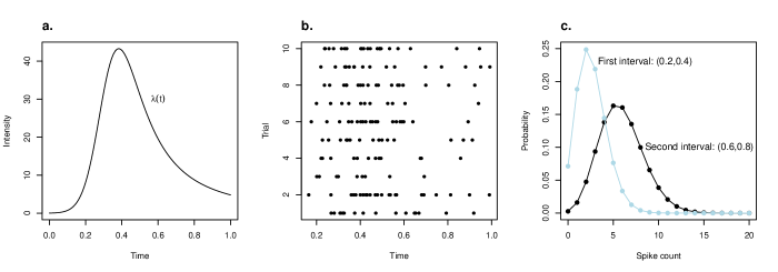
Figure 1: A first example of a point process: the Inhomogeneous Poisson Process (IPP) as a model for spike trains. a. The neuron is assumed to respond to stimulation at a varying rate over time. The latent rate is described by an intensity function, $\lambda(t)$ b. Spikes are stochastic: here we simulated spike trains from an IPP with intensity $\lambda(t)$. Different trials correspond to different realisations. Note that a given spike train can be seen simply as a set of points in $(0,1)$. c. The defining property of the IPP is that spike counts in a given interval follow a Poisson distribution. Here we show the probability of observing a certain number of spikes in two different time intervals.

(a) The latent intensity function $\lambda(x,y)$ controls how many points will fall on average in a certain spatial area. Higher intensities are in lighter shades of blue.

(b) Four samples from an IPP with the intensity function shown in the left-hand panel.

Figure 2: The spatial IPP is a mathematically straightforward extension to the temporal IPP introduced in Figure 1. The main ingredient is a spatial intensity function $\lambda(x,y)$. The IPP produces random point sets, as in the lower panel. When analysing point data, the goal is usually to recover the latent intensity function from such samples.

2.2 The point of point processes

Given a point set, the most natural question to ask is, generally, “what latent intensity function could have generated the observed pattern?” Indeed, we argue that a lot of very specific research questions are actually special cases of this general problem.

For mathematical convenience, we will from now on focus on the log-intensity function $\eta(x,y)=\log\lambda\left(x,y\right)$. The reason this is more convenient is that $\lambda\left(x,y\right)$ cannot be negative—and we are not expecting a negative number of points (fixations)—whereas $\eta\left(x,y\right)$, on the other hand, can take any value whatever, from minus to plus infinity.

At this point we need to introduce the notion of spatial covariate, which are directly analoguous to covariates in linear models. In statistical parlance, the response is what we are interested in predicting, and covariates is what we use to predict the response with. In the case of point processes covariates are often spatial functions too.

One of the classical questions in the study of overt attention is the role of low-level cues in attracting gaze (i.e. visual saliency). Among low-level cues, local contrast may play a prominent role, and it is a classical finding that observers tend to be more interested in high-contrast regions when viewing natural images, e.g. (Rajashekar et al.,, 2007).

Imagine that our point set $\mathbf{F}=\left\{\left(x_{1},y_{1}\right),\ldots,\left(x_{n},y_{n}\right)\right\}$ represents observed fixation locations on a certain image, and we assume that these fixation locations were generated by an IPP with log-intensity function $\eta\left(x,y\right)$. We suppose that the value of $\eta\left(x,y\right)$ at location $x,y$ has something to do with the local contrast $c(x,y)$ at the location. In other words, the image contrast function $c(x,y)$ will enter as a covariate in our model. The simplest way to do so is to posit that $\eta\left(x,y\right)$ is a linear function of $c(x,y)$, i.e.:

$$\eta\left(x,y\right)=\beta_{c}\times c(x,y)+\beta_{0}$$ (1)

We have introduced two free parameters, $\beta_{c}$ and $\beta_{0}$, that will need to be estimated from the data. $\beta_{c}$ is the more informative of the two: for example, a positive value indicates that high contrast is predictive of high intensity, and a nearly-null value indicates that contrast is not related to intensity (or at least not monotonically). We will return to this idea below when we consider analysing the output of low-level saliency models.

Another example that will come up in our analysis is the well-documented issue of the “centrality bias”, whereby human observers in psychophysical experiments in front of a centrally placed computer screen tend to fixate central locations more often regardless of what they are shown (Tatler,, 2007). Again this has an influence on the intensity function that needs to be accounted for. One could postulate another spatial (intrinsic) covariate, $d\left(x,y\right)$, representing the distance to the centre of the display: e.g., $d(x,y)=\sqrt{x^{2}+y^{2}}$ assuming the centre is at $(0,0)$. As in Equation (1), we could write

$$\eta\left(x,y\right)=\beta_{d}\times d(x,y)+\beta_{0}$$

However, in a given image, both centrality bias and local contrast will play a role, resulting in:

$$\eta\left(x,y\right)=\beta_{d}\times d(x,y)+\beta_{c}\times c(x,y)+\beta_{0}$$ (2)

The relative contribution of each factor will be determined by the relative values of $\beta_{d}$ and $\beta_{c}$. Such additive decompositions will be central to our analysis, and we will cover them in much more detail below.

3 Case study: Analysis of low-level saliency models

If eye movement guidance is a relatively inflexible system which uses local image cues as heuristics for finding interesting places in a stimulus, then low-level image cues should be predictive of where people look when they have nothing particular to do. This has been investigated many times (see Schütz et al.,, 2011), and there are now many datasets available of “free-viewing” eye movements in natural images (Van Der Linde et al.,, 2009; Torralba et al.,, 2006). Here we use the dataset of Kienzle et al., (2009) because the authors were particularly careful to eliminate a number of potential biases (photographer’s bias, among other things).

In Kienzle et al., (2009), subjects viewed photographs taken in a zoo in Southern Germany. Each image appeared for a short, randomly varying duration of around 2 sec. Subjects were instructed to “look around the scene”, with no particular goal given. The raw signal recorded from the eye-tracker was processed to yield a set of saccades and fixations, and here we focus only on the latter. We have already mentioned in the introduction that such data are often analysed in terms of a patch classification problem: can we tell between fixated and non-fixated image patches based on their content? We now explain how to replicate the main features of a such an analysis in terms of the point process framework.

3.1 Understanding the role of covariates in determining fixated locations

To be able to move beyond the basic statement that local image cues somehow correlate with fixation locations, it is important that we clarify how covariates could enter into the latent intensity function. There are many different ways in which this could happen, with important consequences for the modelling. Our approach is to build a model gradually, starting from simplistic assumptions and introducing complexity as needed.

To begin with we imagine that local contrast is the only cue that matters. A very unrealistic but drastically simple model assumes that the more contrast there is in a region, the more subjects’ attention will be attracted to it. In our framework we could specify this model as:

$$\eta\left(x,y\right)=\beta_{0}+\beta_{1}c(x,y)$$

However, surely other things besides contrast matters - what about average luminance, for example? Couldn’t brighter regions attract gaze?

This would lead us to expand our model to include luminance as another spatial covariate, so that the log-intensity function becomes:

$$\eta\left(x,y\right)=\beta_{0}+\beta_{1}c(x,y)+\beta_{2}l(x,y)$$

in which $l(x,y)$ stands for local luminance. But perhaps edges matter, so why not include another covariate corresponding to the output of a local edge detector $e(x,y)$? This results in:

$$\eta\left(x,y\right)=\beta_{0}+\beta_{1}c(x,y)+\beta_{2}l(x,y)+\beta_{3}e(x,y)$$

It is possible to go further down this path, and add as many covariates as one sees fit (although with too many covariates, problems of variable selection do arise, see Hastie et al.,, 2003), but to make our lives simpler we can also rely on some prior work in the area and use pre-existing, off-the-shelf image-based saliency models (Fecteau and Munoz,, 2006). Such models combine many local cues into one interest map, which saves us from having to choose a set of covariates and then estimating their relative weight (although see Vincent et al.,, 2009 for work in a related direction). Here we focus on the perhaps most well-known among these models, described in Itti and Koch, (2001) and Walther and Koch, (2006), although many other interesting options are available (e.g., Bruce and Tsotsos,, 2009, Zhao and Koch,, 2011, or Kienzle et al.,, 2009).

Figure 3: An image from the dataset of Kienzle et al., (2009), along with an “interest map” - local saliency computed according to the Itti-Koch model (Itti and Koch,, 2001; Walther and Koch,, 2006). Fixations made by the subjects are overlaid in red. How well does the interest map characterise this fixation pattern? This question is not easily answered by eye, but may be given a more precise meaning in the context of spatial processes.

The model computes several feature maps (orientation, contrast, etc.) according to physiologically plausible mechanisms, and combines them into one master map which aims to predict what the interesting features in image $i$ are. For a given image $i$ we can obtain the interest map $m_{i}\left(x,y\right)$ and use that as the unique covariate in a point process:

$$\eta_{i}\left(x,y\right)=\alpha_{i}+\beta_{i}m_{i}(x,y)$$ (3)

This last equation will be the starting point of our modelling. We have changed the notation somewhat to reflect some of the adjustments we need to make in order to learn anything from applying model to data. To summarise:

• $\eta_{i}(x,y)$ denotes the log-intensity function for image $i$, which depends on the spatial covariate $m_{i}\left(x,y\right)$ that corresponds to the interest map given by the low-level saliency of Itti and Koch, (2001).

• $\beta_{i}$ is an image-specific coefficient that measures to what extent spatial intensity can be predicted from the interest map. $\beta_{i}=0$ means no relation, $\beta_{i}>0$ means that higher low-level saliency is associated on average with more fixations, $\beta_{i}<0$ indicates the opposite - people looked more often at low points of the interest map. We make $\beta_{i}$ image-dependent because we anticipate that how well the interest map predicts fixations depends on the image, an assumption that is borne out, as we will see.

• $\alpha_{i}$ is an image specific intercept. It is required for technical reasons but otherwise plays no important role in our analysis.

We fitted the model given by Equation (3) to a dataset consisting of the fixations recorded in the first 100 images of the dataset of Kienzle et al., (2009, see Fig. reffig:IttiKochSaliencyKienzle). Computational methods are described in the appendix. We obtained a set of posterior estimates for the $\beta_{i}$’s, of which a summary is given in Figure 4.

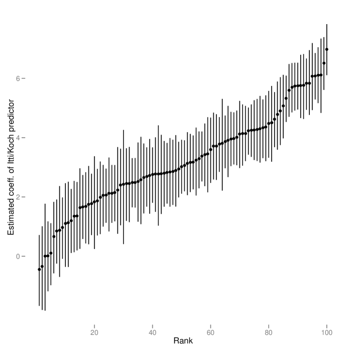
Figure 4: Variability in the predictivity of the Itti-Koch model across images. We estimate $\beta_{i}$ in Equation 3 for 100 different images from the dataset of Kienzle et al., (2009). We plot the sorted mean-a-posteriori estimates along with a 95% Bayesian credible interval. The results show clearly that the “interestingness” given by low-level saliency is of variable value when predicting fixations: for some images $\beta_{i}$ is very close to 0, which indicates that there is no discernible association between low-level saliency and fixation intensity in these images. In other images the association is much stronger.

To make the coefficients shown on Figure 4 more readily interpretable, we have scaled $m_{i}\left(x,y\right)$ so that in each image the most interesting points (according to the Itti-Koch model) have value 1 and the least interesting 0. In terms of the estimated coefficients $\beta_{i}$, this implies that the intensity ratio between a maximally interesting region and a minimally interesting region is equal to $e^{\beta_{i}}$: for example, a value of $\beta_{i}$ of 1 indicates that in image $i$ on average a region with high “interestingness” receives roughly 2.5 more fixations than a region with very low “interestingness”. At the opposite end of the spectrum, in images in which the Itti-Koch model performs very well, we have values of $\beta_{i}\approx 6$, which implies a ratio of 150 to 1 for the most interesting regions compared to the least interesting.

It is instructive to compare the images in which the model does well, to those in which it does poorly. On Figure 5 we show the 8 images with highest $\beta_{i}$ value, and on Figure 6 the 8 images with lowest $\beta_{i}$, along with the corresponding Itti-Koch interest maps. It is evident that, while on certain images the model does extremely well, for example when it manages to pick up the animal in the picture (see the lion in images 52 and 53), in others it gets fooled by high-contrast edges that subjects find highly uninteresting. Foliage and rock seem to be particularly difficult, at least from the limited evidence available here.

Given a larger annotated dataset, it would be possible to confirm whether the model performs better for certain categories of images than others. Although this is outside the scope of the current paper, we would like to point out that the model in Equation (3) can be easily extended for that purpose: If we assume that images are encoded as being either “foliage” or “not foliage”, we may then define a variable $\phi_{i}$ that is equal to 1 if image $i$ is foliage and 0 if not. We may re-express the latent log-intensity as:

$$\eta_{i}\left(x,y\right)=\alpha_{i}+\left(\phi_{i}\gamma+\delta_{i}\right)m_{i}(x,y)$$

which decomposes $\beta_{i}$ as the sum of an image-specific effect ($\delta_{i}$) and an effect of belonging to the foliage category $\left(\gamma\right)$. Having $\gamma<0$ would indicate that pictures of foliage are indeed more difficult on average. We take foliage here only as an illustration of the technique, as it is certainly not the most useful categorical distinction one could make (for a taxonomy of natural images, see Fei-Fei et al.,, 2007, and, e.g., Kaspar and König,, 2011 for a discussion of image categories).

A related suggestion (Torralba et al.,, 2006) is to augment low-level saliency models with some higher-level concepts, adding face detectors, text detectors, or horizon detectors. Within the limits of our framework, a much easier way to improve predictions is to take into account the centrality bias (Tatler and Vincent,, 2009), i.e. the tendency for observers to fixate more often at the centre of the image than around the periphery. One explanation for the centrality bias is that it is essentially a side-effect of photographer’s bias: people are interested in the centre because the centre is where photographers usually put the interesting things, unless they are particularly incompetent. In Kienzle et al., (2009) photographic incompetence was simulated by randomly clipping actual photographs so that central locations were not more likely to be interesting than peripheral ones. The centrality bias persists (see Fig. 7), which shows that central locations are preferred regardless of image content (a point already made in Tatler,, 2007). We can use this fact to make better predictions by making the required modifications to the intensity function.

Before we can explain how to do that, we need to introduce a number of additional concepts. A central theme in the proposed spatial point process framework is to develop tools that help us to understand performance of our models in detail. In the next section we introduce some relatively user-friendly graphical tools for assessing fit. We will also show how one can estimate an intensity function in a non-parametric way, that is, without assuming that the intensity function has a specific form. Nonparametric estimates are important in their own right for visualisation (see for example the right-hand-side of Fig. 7), but also as a central element in more sophisticated analyses.

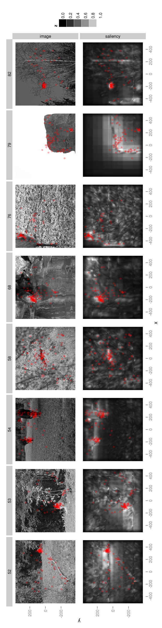
Figure 5: Out of first 100 pictures in the Kienzle et al. dataset, we show the 8 ones in which Itti&Koch interestingness has the strongest link to fixation density (according to the value of $\beta_{i}$ in Equation 3). The I&K interest map is displayed below each image, and fixation locations are in red.

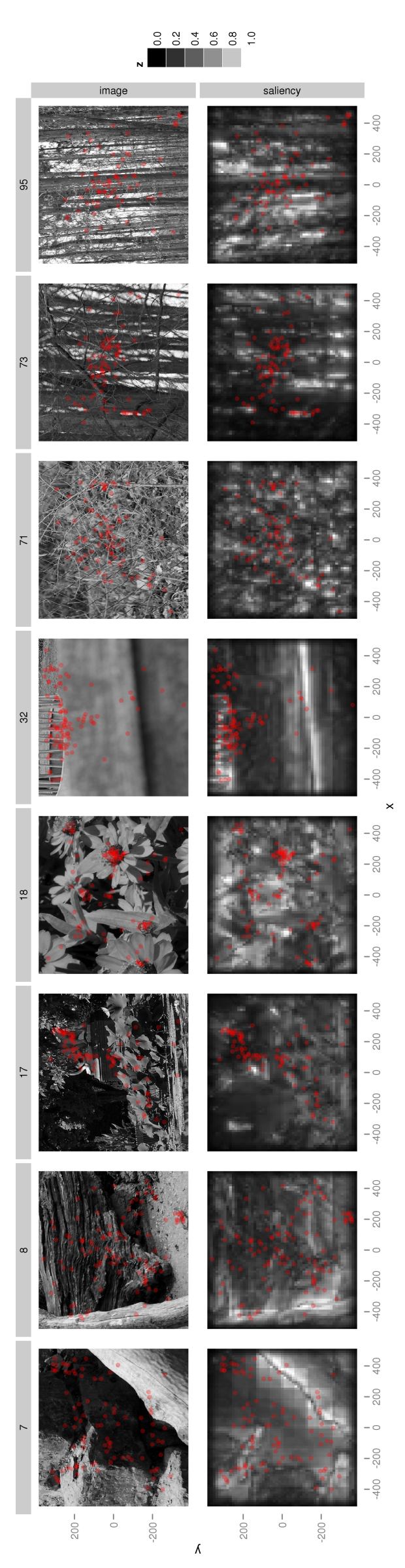
Figure 6: Same as Figure 5 above, but with the 8 images with lowest value for $\beta_{i}$ .

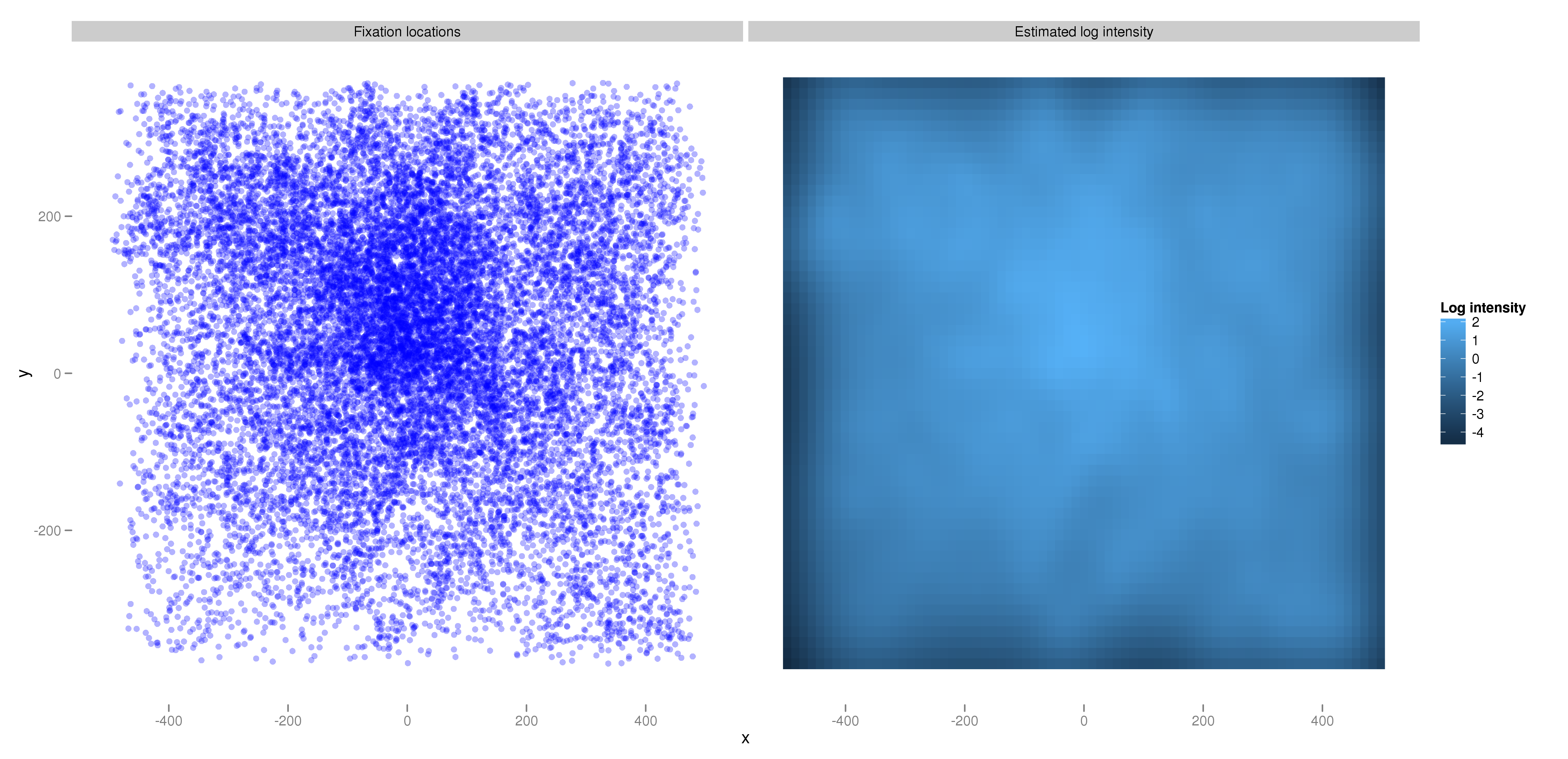
Figure 7: The centrality bias. On the left panel, we plot every fixation recorded in Kienzle et al., (2009). On the right, a non-parametric Bayesian estimate of the intensity function. Central locations are much more likely to be fixated than peripheral ones.

3.2 Graphical model diagnostics

Once one has fitted a statistical model to data, one has to make sure the fitted model is actually at least in rough agreement with the data. A good fit alone is not the only thing we require of a model, because fits can in some cases be arbitrarily good if enough free parameters are introduced (see e.g., Bishop,, 2007, ch. 3). But assessing fit is an important step in model criticism (Gelman and Hill,, 2006), which will let us diagnose model failures, and in many cases will enable us to obtain a better understanding of the data itself. In this section we will focus on informal, graphical diagnostics. More advanced tools are described in Baddeley et al., (2005). Ehinger et al., (2009) use a similar model-criticism approach in the context of saliency modelling.

Since a statistical model is in essence a recipe for how the data are generated, the most obvious thing to do is to compare data simulated from the model to the actual data we measured. In the analysis presented above, the assumption is that the data come from a Poisson process whose log-intensity is a linear function of Itti-Koch interestingness:

$$\eta_{i}\left(x,y\right)=\alpha_{i}+\beta_{i}m_{i}(x,y)$$ (4)

For a given image, we have estimated values $\hat{\alpha}_{i},\hat{\beta}_{i}$ (mean a posterior estimate). A natural thing to do is to ask what data simulated from a model with those parameters look like. In Figure 8, we take the image with the maximum estimated value for $\beta_{i}$ and compare the actual recorded fixation locations to four different simulations from an IPP with the fitted intensity function.

What is immediately visible from the simulations is that, while the real data present one strong cluster that also appears in the simulations, the simulations have a higher proportion of points outside of the cluster, in areas far from any actual fixated locations. Despite these problems, the fit seems to be quite good compared to other examples from the dataset: Figure 9 shows two other examples, image 45, which has a median $\beta$ value of about 4, and image 32, which had a $\beta$ value of about 0. In the case of image 32, since there is essentially no relationship between the interestingness values and fixation locations, the best possible intensity function of the form given by Equation (3) is one with $\beta=0$, a uniform intensity function.

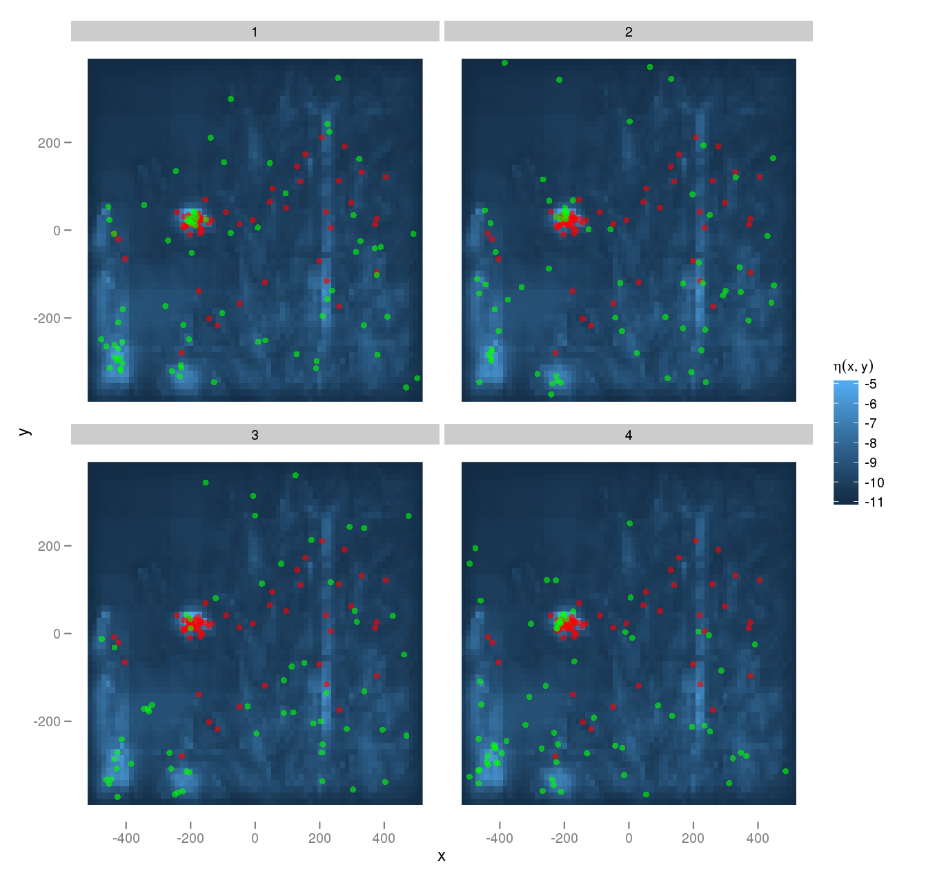
Figure 8: Simulating from a fitted point process model. The fixations on image 82 (rightmost in Figure 5) were fitted with the model given by Equation (3), resulting in an estimated log-intensity $\eta(x,y)$ which is plotted as a heatmap in the background of each panel. In red we plot the actual fixation locations (the same in every of the four panels), and in green simulations from the fitted model, four different realizations, one in each panel.

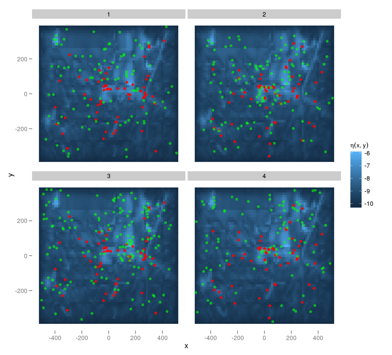
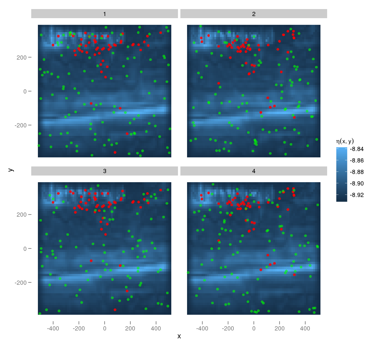
Figure 9: Same as in Figure 8, with the fixations measured on image 45 (left) and 32 (right) of the dataset. The agreement between data and simulations is of distinctly poorer quality than in image 82.

It is also quite useful to inspect some of the marginal distributions. By marginal distributions we mean point distributions that we obtain by merging data from different conditions. In Figure 10, we plot the fixation locations across all images in the dataset. In the lower panel we compare it to simulations from the fitted model, in which we generated fixation locations from the fitted model for each image so as to simulate an entire dataset. This brings to light a failure of the model that would not be obvious from looking at individual images: based on Itti-Koch interestingness alone we would predict a distribution of fixation locations that is almost uniform, whereas the actual distribution exhibits a central bias, as well as a bias for the upper part of the screen.

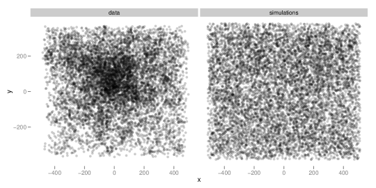
Figure 10: Comparing marginal fixation locations. On the left panel, we plot each fixation location in images 1 to 100 (each dot corresponds to one fixation). On the right panel, we plot simulated fixation locations from the fitted model corresponding to Equation (3). A strong spatial bias is visible in the data, not captured at all by the model.

Overall, the model derived from fitting Equation (3) seems rather inadequate, and we need to account at least for what seems to be some prior bias favouring certain locations. Explaining how to do so requires a short detour through the topic of non-parametric inference, to which we turn next.

3.3 Inferring the intensity function non-parametrically

Consider the data in Figure 7: to get a sense of how much observers prefer central locations relative to peripheral ones, we could define a central region $\mathcal{A}$, count how many fixations fall in it, compared to how many fixations fall outside. From the theoretical point of view, what we are doing is directly related to estimating the intensity function: the expected number of fixations in $\mathcal{A}$ is after all $\int_{\mathcal{A}}\lambda\left(x,y\right)\mbox{d}x\mbox{d}y$, the integral of the intensity function over $\mathcal{A}$. Seen the other way, counting how many sample points are in $\mathcal{A}$ is a way of estimating the integral of the intensity over $\mathcal{A}$.

Modern statistical modelling emphasizes non-parametric estimation. If one is trying to infer the form of an unknown function $f(x)$, one should not assume that $f(x)$ has a certain parametric form unless there is very good reason for this choice (interpretability, actual prior knowledge or computational feasibility). Assuming a parametric form means assuming for example that $f(x)$ is linear, or quadratic: in general it means assuming that $f(x)$ can be written as $f(x)=\phi(x;\beta)$, where $\beta$ is a finite set of unknown parameters, and $\phi\left(x;\beta\right)$ is a family of functions over $x$ parameterised by $\beta$. Nonparametric methods make much weaker assumptions, usually assuming only that $f$ is smooth at some spatial scale.

We noted above that estimating the integral of the intensity function over a spatial region could be done by counting the number of points the region contains. Assume we want to estimate the intensity $\lambda(x,y)$ at a certain point $x_{0},y_{0}$. We have a realisation $S$ of the point process (for example a set of fixation locations). If we assume that $\lambda(x,y)$ is spatially smooth, it implies that $\lambda(x,y)$ varies slowly around $x_{0},y_{0}$, so that we may consider it roughly constant in a small region around $x_{0},y_{0}$, for instance in a circle of radius $r$ around $(x_{0},y_{0})$. Call this region $\mathcal{C}_{r}$ - the integral of the intensity function over $\mathcal{C}_{r}$ is related to the intensity at $(x_{0}$,$y_{0}$) in the following way:

$$\int_{\mathcal{C}_{r}}\lambda(x,y)\mbox{d}x\mbox{d}y\approx\int_{\mathcal{C}_{r}}\lambda\left(x_{0},y_{0}\right)\mbox{d}x\mbox{d}y=\lambda\left(x_{0},y_{0}\right)\times\int_{\mathcal{C}_{r}}\mbox{d}x\mbox{d}y$$

$\int_{\mathcal{C}_{r}}\mbox{d}x\mbox{d}y$ is just the area of circle $\mathcal{C}_{r}$, equal to $\pi r$. Since we can estimate $\int_{\mathcal{C}_{r}}\lambda(x,y)\mbox{d}x\mbox{d}y$ via the number of points in $\mathcal{C}_{r}$, it follows that we can estimate $\lambda(x_{0},y_{0})$ via:

$$\hat{\lambda}\left(x_{0},y_{0}\right)=\frac{\left|S\cap\mathcal{C}_{r}\right|}{\pi r}$$

$\left|S\cap\mathcal{C}_{r}\right|$ is the cardinal of the intersection of the point set $S$ and the circle $\mathcal{C}_{r}$ (note that they are both sets), shorthand for “number of points in $S$ that are also in $\mathcal{C}_{r}$”.

What we did for $(x_{0},y_{0})$ remains true for all other points, so that a valid strategy for estimating $\lambda(x,y)$ at any point is to count how many points in $S$ are in the circle of radius $r$ around the location. The main underlying assumption is that $\lambda\left(x,y\right)$ is roughly constant over a region of radius $r$. This method will be familiar to some readers in the context of non-parametric density estimation, and indeed it is almost identical. It is a perfectly valid strategy, detailed in Diggle, (2002), and its only major shortcoming is that the amount of smoothness (represented by $r$) one arbitrarily uses in the analysis may change the results quite dramatically (see Figure 11). Although it is possible to also estimate $r$ from the data, in practice this may be difficult (see Illian et al.,, 2008, Section 3.3).

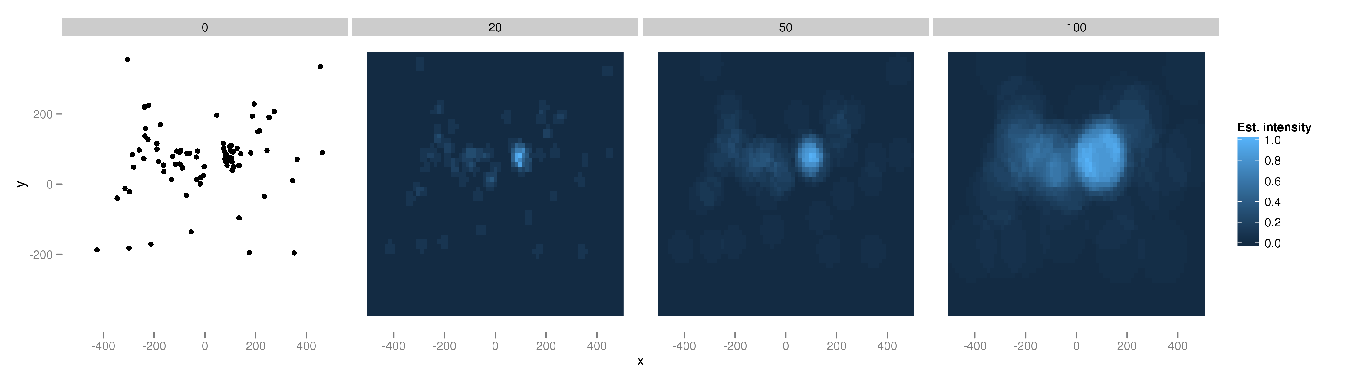
Figure 11: Nonparametric estimation of the intensity function using a moving window. The data are shown on the leftmost panel. The intensity function at $(x,y)$ is estimated by counting how many points are within a radius $r$ of $(x,y)$. We show the results for $r=20,50,100$. Note that with $r\rightarrow 0$ we get back the raw data. For easier visualization, we have scaled the intensity values such that the maximum intensity is 1 in each panel.

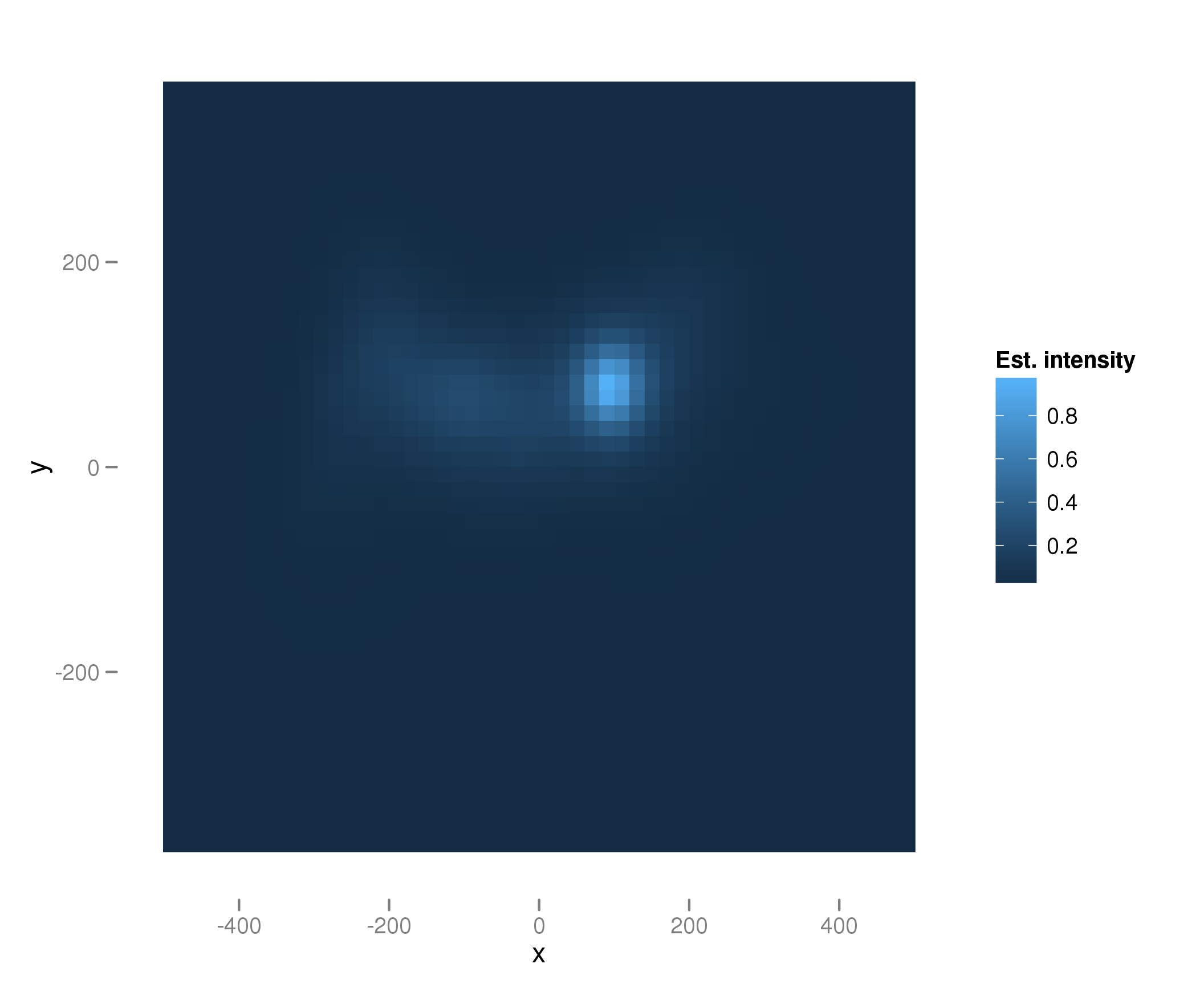
Figure 12: Nonparametric Bayesian estimation of the intensity function. We use the same data as in Figure 11. Inference is done by placing a Gaussian process prior on the log-intensity function, which enforces smoothness. Hyperparameters are integrated over. See text and appendix 5.2 for details.

There is a Bayesian alternative: put a prior distribution on the intensity $\lambda$ and base the inference on the posterior distribution of $\lambda(x,y)$ given the data, with

$$p(\lambda|S)\propto p(S|\lambda)p(\lambda)$$

as usual. We can use the posterior expectation of $\lambda(x,y)$ as an estimator (the posterior expectation is the mean value of $\lambda(x,y)$ given the data), and the posterior quantiles give confidence intervals. The general principles of Bayesian statistics will not be explained here, the reader may refer to Kruschke, (2010) or any other of the many excellent textbooks on Bayesian statistics for an introduction.

To be more precise, the method proceeds by writing down the very generic model:

$$\log\lambda\left(x,y\right)=f(x,y)+\beta_{0}$$

and effectively forces $f(x,y)$ to be a relatively smooth function, using a Gaussian Process prior. Exactly how this is achieved is explained in Appendix 5.2, but roughly, Gaussian Processes let one define a probability distribution over functions such that smooth functions are much more likely than non-smooth functions. The exact spatial scale over which the function is smooth is unknown but can be averaged over.

To estimate the intensity function of one individual point process, there is little cause to prefer the Bayesian estimate over the classical non-parametric estimate we described earlier. As we will see however, using a prior that favours smooth functions becomes invaluable when one considers multiple point processes with shared elements.

3.4 Including a spatial bias, and looking at predictions for new images

We have established that models built from interest maps do not fit the data very well, and we have hypothesized that one possible cause might be the presence of a spatial bias. Certain locations might be fixated despite having relatively uninteresting contents. A small modification to our model offers a solution: we can hypothesize that all latent intensity functions share a common component. In equation form:

$$\eta_{i}\left(x,y\right)=\alpha_{i}+\beta_{i}m_{i}(x,y)+g(x,y)$$ (5)

As in the previous section, we do not force $g(x,y)$ to take a specific form, but only assume smoothness. Again, we use the first 100 images of the dataset to estimate the parameters. The estimated spatial bias is shown on Figure 13. It features the centrality bias and the preference for locations above the midline that were already visible in the diagnostics plot of Section 3.2 (Fig. 10).

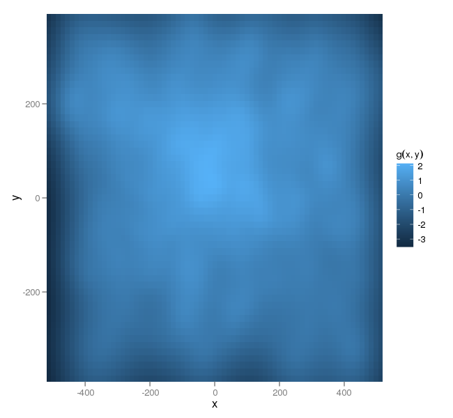
Figure 13: Estimated spatial bias $g(x,y)$ (Eq. 5).

From visual inspection alone it appears clear that including a spatial bias is necessary, and that the model with spatial bias offers a significant improvement over the one that does not. However, things are not always as clear-cut, and one cannot necessarily argue from a better fit that one has a better model. There are many techniques for statistical model comparison, but given sufficient data the best is arguably to compare the predictive performance of the different models in the set (see Pitt et al.,, 2002, and Robert,, 2007, ch. 7 for overviews of model comparison techniques). In our case we could imagine two distinct prediction scenarios:

1. For each image, one is given, say, 80% of the recorded fixations, and must predict the remaining 20%.

2. One is given all fixation locations in the first $n$ images, and must predict fixations locations in the next $k$.

To use low-level saliency maps in engineering applications (Itti,, 2004), what is needed is a model that predicts fixation locations on arbitrary images—i.e. the model needs to be good at the second prediction scenario outlined above. The model is tuned on recorded fixations on a set of training images, but to be useful it must make sensible predictions for images outside the original training set.

From the statistical point of view, there is a crucial difference between prediction problems (1) and (2) above. Problem (1) is easy: to make predictions for the remaining fixations on image $i$, estimate $\beta_{i}$ and $\alpha_{i}$ from the available data, and predict based on the estimated values (or using the posterior predictive distribution). Problem (2) is much more difficult: for a new image $j$ we have no information about the values of $\beta_{j}$ or $\alpha_{j}$. In other words, in a new image the interest map could be very good or worthless, and we have no way of knowing that in advance.

We do however have information about what values $\beta_{j}$ and $\alpha_{j}$ are likely to take from the estimated values for the images in the training set. If in the training set nearly all values $\beta_{1},\beta_{2},\ldots,\beta_{n}$ were above 0, it is unlikely that $\beta_{j}$ will be negative. We can represent our uncertainty about $\beta_{j}$ with a probability distribution, and this probability distribution may be estimated from the estimated values for $\beta_{1},\beta_{2},\ldots,\beta_{n}$. We could, for example, compute their mean and standard deviation, and assume that $\beta_{j}$ is Gaussian distributed with this particular mean and standard deviation. Another way, which we adopt here, is to use a kernel density estimator so as not to impose a Gaussian shape on the distribution.

As a technical aside: for the purpose of prediction the intercept $\alpha_{j}$ can be ignored, as its role is to modulate the intensity function globally, and it has no effect on where fixations happen, simply on how many fixations are predicted. Essentially, since we are interested in fixation locations, and not in how many fixations we get for a given image, we can safely ignore $\alpha_{i}.$ A more mathematical argument is given in Appendix 5.3.2.

Thus how to predict? We know how to predict fixation locations given a certain value of $\beta_{j}$, as we saw earlier in Section 3.2. Since $\beta_{j}$ is unknown we need to average over our uncertainty. A recipe for generating predictions is to sample a value for $\beta_{j}$ from $p(\beta_{j})$, and conditional on that value, sample fixation locations. Please refer to Figure 14 for an illustration.

Figure 14: Predictions for a novel image. The latent intensity function in Equation 5 has two important components: the interest map $m(x,y)$, shown here in panel (a) for image 103, and a general spatial component $g(x,y)$, shown in (b). Image 103 does not belong to the training set, and the value of $\beta_{103}$ is therefore unknown: we do not know if $m(x,y)$ will be a strong predictor or not, and must therefore take this uncertainty into account. Uncertainty is represented by the distribution the $\beta$ coefficient takes over images, and we can estimate this distribution from the estimated values from the training set. In (c) we show those values as dashes, along with a kernel density estimate. Conditional on a given value for $\beta_{103}$, our predictions come from a point process with log-intensity function given by $\beta_{103}m_{103}\left(x,y\right)+g\left(x,y\right)$: in (d), we show the intensity function for $\beta_{103}=0,3,6$. In (e), we show simulations from the corresponding point processes (conditional on $n=100$ fixations, see 5.3.2). In general the strategy for simulating from the predictive distribution will be to sample a value of $\beta$ from $p(\beta)$, and sample from the corresponding point process as is done here.

In Figure 15 we compare predictions for marginal fixation locations (over all images), with and without a spatial bias term. We simulated fixations from the predictive distribution for images 101 to 200. We plot only one simulation, since all simulations yield for all intents and purposes the same result: without a spatial bias term, we replicate the problem seen in Figure 10. We predict fixations distributed more or less uniformly over the monitor. Including a spatial bias term solves the problem.

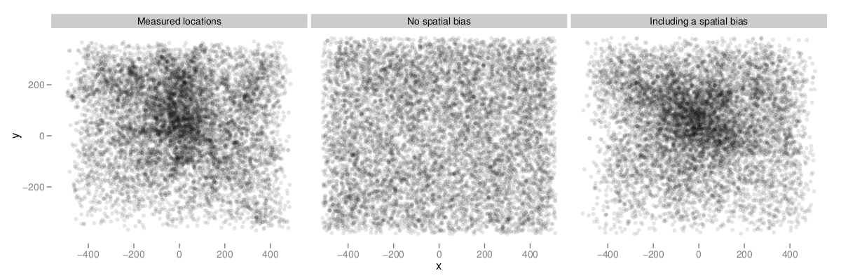
Figure 15: Predicting marginal fixation locations. In the first panel we plot the location of all fixations for images 101 to 200. In the second panel we plot simulated fixation locations for the same images from the naive model of Equation 3. In the second panel we plot simulated fixation locations for the same images from the model of Equation 13, which includes a spatial bias. Note that these are predicted fixation locations for entirely new images, and not a fit. Including a spatial bias improves predictions enormously.

What about predictions for individual images? Typically in vision science we are attempting to predict a one-dimensional quantity: for example, we might have a probability distribution for somebody’s contrast threshold. If this probability distribution has high variance, our predictions for any individual trial or the average of a number of trials are by necessity imprecise. In the one-dimensional case it is easy to visualise the degree of certainty by plotting the distribution function, or providing a confidence interval. In a point process context, we do not deal with one-dimensional quantities: if the goal is to predict where 100 fixations on image $j$ might fall, we are dealing with a 200 dimensional space—100 points times 2 spatial dimensions. A maximally confident prediction would be represented by a probability distribution that says that all points will be at a single location. A minimally confident prediction would be represented by the uniform distribution over the space of possible fixations, saying that all possible configurations are equally likely. Thus the question that needs to be addressed is, where do the predictions we can make from the Itti-Koch model fall along this axis?

It is impossible to provide a probability distribution, or to report confidence intervals. A way to visualise the amount of uncertainty we have is by drawing samples from the predictive probability distribution, to see if the samples vary a lot. Each sample is a set of a 100 points: if we notice for example that over 10 samples all the points in each sample systematically cluster at a certain location, it indicates that our predictive distribution is rather specific. If we see at lot of variability across samples, it is not. This mode of visualisation is better adapted to a computer screen than to be printed on paper, but for five examples we show eight samples in Figure 16.

To better understand the level of uncertainty involved, imagine that the objective is to perform (lossy) image compression. We picked this example because saliency models are sometimes advocated in the compression context (Itti,, 2004). Lossy image compression works by discarding information and hoping people will not notice. The promise of image-based saliency models is that if we can predict what part of an image people find interesting, we can get away with discarding more information where people will not look. Let us simplify the problem and assume that either we compress an area or we do not. The goal is to find the largest possible section of the image we can compress, under the constraint that if a 100 fixations are made in the image, less than 5 fall in the compressed area (with high probability). If the predictive distribution is uniform, we can afford to compress less than 5% of the area of the image. A full formalisation of the problem for other distributions is rather complicated, and would carry us outside the scope of this introduction, but looking at the examples of Figure 16 it is not hard to see qualitatively that for most images, the best area we can find will be larger than 5% but still rather small: in the predictive distributions, points have a tendency of falling in most places except around the borders of the screen.

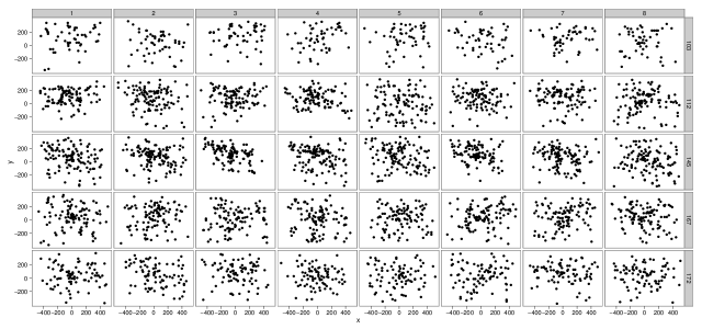
Figure 16: Samples from the predictive distributions for the model including spatial bias. We picked five images at random, and generated 8 samples from the predictive distribution from each, using the technique outlined in Figure 14. Each row corresponds to one image, with samples along the columns. This lets us visualise the uncertainty in the predictive distributions, see text.

The reason we see such imprecision in the predictive distributions is essentially because we have to hedge our bets: since the value of $\beta$ varies substantially from one image to another, our predictions are vague by necessity. In most cases, models are evaluated in terms of average performance (for example, average AUC performance over the dataset). The above results suggest that looking just at average performance is insufficient. A model that is consistenly mediocre may for certain applications be preferable than a model that is occasionally excellent but sometimes terrible. If we cannot tell in advance when the latter model does well, our predictions about fixation locations may be extremely imprecise.

3.5 Dealing with non-stationarities: dependency on the first fixation

One very legitimate concern with the type of models we have used so far is the independence assumption embedded into the IPP: all fixations are considered independent of each other. Since successive fixations tend to occur close to one another, we know that the independence assumption is at best a rough approximation to the truth. There are many examples of models in psychology that rather optimistically assume independence and thus neglect nonstationarities: when fitting psychometric functions for example, one conveniently ignores sequential dependencies, learning, etc. but see Fründ et al., (2011) or Schönfelder and Wichmann (in press). One may argue, however, that models assuming independence are typically simpler, and therefore less likely to overfit, and that the presence of dependencies effectively acts as an additional (zero-mean) noise source that does not bias the results. This latter assumption requires to be explicitly checked, however. In this section we focus specifically on a source of dependency that could bias the results (dependency on the first fixation), and show that (a) our models can amended to take this dependency into account, (b) that the dependency indeed exists, although (c) results are not affected in a major way. We conclude with a discussion of dependent point processes and some pointers to the relevant literature.

In the experiment of Kienzle et al., (2009), subjects only had a limited amount of time to look at the pictures: generally less than 4 seconds. This does not always allow enough time to explore the whole picture, so that subjects may have only explored a part of the picture limited to an certain area around the initial fixation. As explained on Figure 17, such dependence may cause us to underestimate the predictive value of a saliency map. Supposing that fixations are indeed driven by the saliency map, there might be highly salient regions that go unexplored because they are too far away from the initial fixation. In a model such as we have used so far, this problem would lead to under-estimating the $\beta$ coefficients.

As with spatial bias, there is again a fairly straightforward solution: we add an additional spatial covariate, representing distance to the original fixation. The log-intensity functions are now modelled as:

$$\eta_{ij}\left(x,y\right)=\alpha_{ij}+\beta_{i}m_{i}(x,y)+\gamma d_{ij}(x,y)+\nu c(x,y)$$ (6)

Introducing this new spatial covariate requires some changes. Since each subject started at a different location, we have one point process per subject and per image, and therefore the log-intensity functions $\eta_{ij}$ are now indexed both by image $i$ and subject $j$ (and we introduce the corresponding intercepts $\alpha_{ij}$). The covariate $d_{ij}\left(x,y\right)$ corresponds to the Euclidean distance to the initial fixation, i.e. if the initial fixation of subject $j$ on image $i$ was at $x=10,y=50$, $d_{ij}\left(x,y\right)=\sqrt{\left(x-10\right)^{2}+\left(y-50\right)^{2}}$. The coefficient $\gamma$ controls the effect of the distance to the initial fixation: a negative value of $\gamma$ means that intensity decreases away from the initial location, or in other words that fixations tend to stay close to the initial location. For the sake of computational simplicity, we have replaced the non-parametric spatial bias term $g(x,y)$ with a linear term $\nu c(x,y)$ representing an effect of the distance to the center ($c(x,y)=\sqrt{x^{2}+y{}^{2}}$). Coefficient $\nu$ plays a role similar to $\gamma$: a negative value for $\nu$ indicates the presence of a centrality bias. We have scaled $c$ and $d_{ij}$ so that a distance of 1 corresponds to the width of the screen. In this analysis we exclude the initial fixations from the set of fixations, they are used only as covariates. The model does not have any non-parametric terms, so that we can estimate the coefficients using maximum likelihood (standard errors are estimated from the usual normal approximation at the mode).

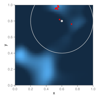
Figure 17: Dependence on the initial fixation location: a potential source of bias in estimation? We show here a random saliency map, and suppose that fixation locations depend on saliency but are constrained by how far away they can move from the original fixation location. The original fixation is in grey, the circle shows a constraint region and the other points are random fixations. The area at the bottom half of the picture is left unexplored not because it is not salient but because it is too far away from the original fixation location. Such dependencies on the initial location may lead to an underestimation of the role of saliency. We describe in the text a method for overcoming the problem.

Again we use the first 100 images in the set to estimate the parameters, and keep the next 100 for model comparison. The fitted coefficient for distance to the initial location is $\hat{\gamma}=-3.2$ (std. err 0.1), and for distance to the center we find $\hat{\nu}=-1.6$ (std. err. 0.1). The value of $\gamma$ indicates a clear dependency on initial location: everything else being equal, at a distance of half the width of the screen the intensity has dropped by a factor 5. To see if the presence of this dependency induces a bias in the estimation of coefficients for the saliency map, we also fitted the model without the initial location term (setting $\gamma$ to 0).

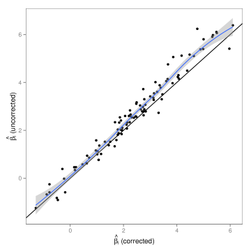
Figure 18: Effect of correcting for dependence on the initial fixation location (see Fig. 17). We compare the estimated value of $\beta_{i}$ using the model of Equation 6, to coefficients estimated from a constrained model that does not include the initial fixation as a covariate. The dots are coefficient pairs corresponding to an image, and in blue we have plotted a trend line. The diagonal line corresponds to equality. Although we do find evidence of dependence on initial fixation location (see text), it does not seem to cause any estimation bias: if anything the coefficients associated with saliency are slightly higher when estimated by the uncorrected model.

We compared the estimated values for $\beta_{i}$ in both models, and show the results on Figure 18: the differences are minimal, although as we have argued there is certainly some amount of dependence on the initial fixation. The lack of an observed effect on the estimation of $\beta$ is probably due to the fact that different observers fixate initially in different locations, and that the dependency effectively washes out in the aggregate. An interesting observation is that in the reduced model the coefficient associated with distance to the center is estimated at -4.1 (std. err. 0.1), which is much larger than when distance to initial fixation is included as a covariate. Since initial fixations are usually close to the center, being close to the center is correlated with being close to the initial fixation location, and part of the centrality bias observed in the dataset might actually be better recast as dependence on the initial location.

In this we have managed to capture a source of dependence between fixations, while seemingly still saving the IPP assumption. We have done so by positing conditional independence: in our improved model all fixations in a sequence are independent given the initial one. An alternative is to drop the independence assumption altogether and use dependent point process models, in which the location of each point depends on the location of its neighbours. These models are beyond the scope of this paper, but they are discussed extensively in Diggle, (2002) and Illian et al., (2008), along with a variety of non-parametric methods that can diagnose interactions.

4 Discussion

We introduced spatial point processes, arguing that they provide a fruitful statistical framework for the analysis of fixation locations and patterns for researchers interested in eye movements. In our exposition we analyzed a low-level saliency model by Itti and Koch, (2001), and we were able to show that—although the model had predictive value on average—it had varying usefulness from one image to another. We believe that the consequences of this problem for prediction are under-appreciated: as we stated in Section 3.4, when trying to predict fixations over an arbitrary image, this variability in quality of the predictor leads to predictions that are necessarily vague. Although insights like this one could be arrived at starting from other viewpoints, they arise very naturally from the spatial point process framework presented here. Indeed, older methods of analysis can be seen as approximations to point process model, as we shall see below.

Owing to the tutorial nature of the material, there are some important issues we have so far set swept under the proverbial rug. The first is the choice of log-additive decompositions: are there other options, and should one use them? The second issue is that of causality (Henderson,, 2003): can our methods say anything about what drives eye movements? Finally, we also need to point out that the scope of point process theory is more extensive than what we have been able to explore in this article, and the last part of the discussion will be devoted to other aspects of the theory that could be of interest to eye movement researchers.

4.1 Point processes versus other methods of analysis

In Section 1.2, we described various methods that have been used in the analysis of fixation locations. Many treat the problem of determining links between image covariates and fixation locations as a patch classification problem: one tries to tell from the contents of an image patch whether it was fixated or not. In the appendix (Section 5.5.1), we show that patch classification has strong ties to point process models, and under some specific forms can be seen as an approximation to point process modelling. In a nutshell, if one uses logistic regression to discriminate between fixated and non-fixated patches, then one is effectively modelling an intensity function. This fact is somewhat obscured by the way the problem is usually framed, but comes through in a formal analysis a bit too long to be detailed here. This result has strong implications for the logic of patch classification methods, especially regarding the selection of control patches, and we encourage interested readers to take a look at Section 5.5.1. Point process theory also allows for a rigorous examination of earlier methods. We take a look in the appendix at AROC values and area counts, two metrics that have been used often in assessing models of fixations. We ask for instance what the ideal model would be, according to the AROC metric, if fixations come from a point process with a certain intensity function. The answer turns out to depend on how the control patches are generated, which is rather crucial to the correct interpretation of the AROC metric. This result and related ones are proved in Section 5.5.2.

We expect that more work will uncover more links between existing methods and the point process framework. One of the benefits of thinking in terms of the more general framework is that many results have already been proven, and many problems have already been solved. We strongly believe that the eye movement community will be able to benefit from the efforts of others who work on spatial data.

4.2 Decomposing the intensity function

Throughout the article we have assumed a log-additive form for our models, writing the intensity function as

$$\lambda\left(x,y\right)=\exp\left(\sum\alpha_{i}v_{i}(x,y)\right)$$ (7)

for a set of covariates $v_{1},\ldots,v_{n}$. This choice may seem arbitrary - for example, one could use

$$\lambda\left(x,y\right)=\sum\alpha_{i}v_{i}(x,y)$$ (8)

a type of mixture model similar to those used in Vincent et al., (2009). Since $\lambda$ needs to be always positive, we would have to assume restrictions on the coefficients, but in principle this decomposition is just as valid. Both (7) and (8) are actually special cases of the following:

$$\lambda\left(x,y\right)=\Phi\left(\sum\alpha_{i}v_{i}(x,y)\right)$$

for some function $\Phi$ (analoguous to the inverse link function in Generalised Linear Models, see McCullagh and Nelder,, 1989). In the case of Equation 7 we have $\Phi\left(x\right)=\exp\left(x\right)$ and in the case of 8 we have $\Phi\left(x\right)=x$. Other options are available, for instance Park et al., (2011) use the following function in the context of spike train analysis:

$$\Phi\left(x\right)=\log(\exp\left(x\right)+1)$$

which approximates the exponential for small values of $x$ and the identity for large ones. Single-index models treat $\Phi$ as an unknown and attempt to estimate it from the data (McCullagh and Nelder,, 1989). From a practical point of view the log-additive form we use is the most convenient, since it makes for a log-likelihood function that is easy to compute and optimise, and does not require restrictions on the space of parameters. From a theoretical perspective, the log-additive model is compatible with a view that sees the brain as combining multiple interest maps $v_{1},v_{2},...$ into a master map that forms the basis of eye movement guidance. The mixture model implies on the contrary that each saccade comes from a roll of dice in which one chooses the next fixation according to one of the $v_{i}$’s. Concretely speaking, if the different interest maps are given by, e.g. contrast and edges, then each saccade is either contrast-driven with a certain probability or on the contrary edges-driven.

We do not know which model is the more realistic, but the question could be addressed in the future by fitting the models and comparing predictions. It could well be that the situation is actually even more complex, and that the data are best described by both linear and log-linear mixtures: this would be the case, for example, if occasional re-centering saccades are interspersed with saccades driven by an interest map.

4.3 Causality

We need to stress that the kind of modelling we have done here does not address causality. The fact that fixation locations can be predicted from a certain spatial covariate does not imply that the spatial covariate causes points to appear. To take a concrete example, one can probably predict the world-wide concentration of polar bears from the quantities of ice-cream sold, but that does not imply that low demand for ice-cream causes polar bears to appear. The same caveat apply in spatial point process models as in regression modelling, see Gelman and Hill, (2006). Regression modelling has a causal interpretation only under very restrictive assumptions.

In the case of determining the causes of fixations in natural images, the issue may actually be a bit muddled, as different things could equally count as causing fixations. Let us go back to polar bears and assume that, while rather indifferent to ice cream, they are quite partial to seals. Thus, the presence of seals is likely to cause the appearance of polar bears. However, due to limitations inherent to the visual system of polar bears, they cannot tell between actual seals and giant brown slugs. The presence of giant brown slugs then also causes polar bears to appear. Both seals and giant brown slugs are valid causes of the presence of polar bears, in the counterfactual sense: no seal, no polar bear, no slug, no polar bear either. A more generic description at the algorithmic level is that polar bears are drawn to anything that is brown and has the right aspect ratio. At a functional level, polar bears are drawn to seals because that is what the polar bear visual system is designed to do.

The same goes for saccadic targeting: an argument is sometimes made that fixated and non-fixated patches only differ in some of their low-level statistics because people target objects, and the presence of objects tend to cause these statistics to change (Nuthmann and Henderson,, 2010). While the idea that people want to look at objects is a good functional account, at the algorithmic level they may try to do so by targeting certain local statistics. There is no confounding in the usual sense, since both accounts are equally valid but address different questions: the first is algorithmic (how does the visual system choose saccade targets based on an image?) and the other one teleological (what is saccade targeting supposed to achieve?). Answering either of these questions is more of an experimental problem than one of data analysis, and we cannot—and do not want to—claim that point process modelling is able to provide anything new in this regard.

4.4 Scope and limitations of point processes

Naturally, there is much we have left out, but at least we would like to raise some of the remaining issues. First, we have left the temporal dimension completely out of the picture. Nicely, adding a temporal dimension in point process models presents no conceptual difficulty; and we could extend the analyses presented here to see in detail whether, for example, low-level saliency predicts earlier fixations better than later ones. We refer the reader to Rodrigues and Diggle, (2012) and Zammit-Mangion et al., (2012) for recent work in this direction.

Second, in this work we have considered that a fixation is nothing more than a dot: it has spatial coordinates and nothing more. Of course, this is not true: a fixation lasted a certain time, during which particular fixational eye movements occured, etc. Studying fixation duration is an interesting topic in its own right, because how long one fixates might be tied to the cognitive processes at work in a task (Nuthmann et al.,, 2010). There are strong indications that when reading, gaze lingers longer on parts of text that are harder to process. Among other things, the less frequent a word is, the longer subjects tend to fixate it (Kliegl et al.,, 2006). Saliency is naturally not a direct analogue of word frequency, but one might nonetheless wonder whether interesting locations are also fixated longer. We could take our data to be fixations coupled with their duration, and we would have what is known in the spatial statistics literature as a marked point process. Marked point processes could be of extreme importance to the analysis of eye movements, and we refer the reader to Illian et al., (2009) for some ideas on this issue.

Third, another limitation we need to state is that the point process models we have described here do not deal very well with high measurement noise. We have assumed that what is measured is an actual fixation location, and not a noisy measurement of an actual measurement location. In addition, the presence of noise in the oculomotor system means that actual fixation location may not be the intended one, which of course adds an intractable source of noise to the measurements. Issues do arise when the scale of measurement error is larger than the typical scale at which spatial covariates change. Although there are theoretical solutions to this problem (involving mixture models), they are rather cumbersome from a computational point of view. An less elegant work-around is to blur the covariates at the scale of measurement error.

Finally, representing the data as a set of locations may not always be the most appropriate way to think of the problem. In a visual search task for example, a potentially useful viewpoint would be to think of a sequence of fixations as covering a certain area of the stimulus. This calls for statistical models that address random shapes rather than just random point sets, an area known as stochastic geometry (Stoyan et al.,, 1996), and in which point processes play a central role, too.

5 Appendices

5.1 The messy details of spatial statistics, and how to get around them

The field of applied spatial statistics has evolved into a powerful toolbox for the analysis of eye movements. There are, however, two main hurdles in terms of accessibility. First, compared to eye-movement research, the more traditional application fields (ecology, forestry, epidemiology) have a rather separate set of problems. Consequently, textbooks (e.g., Illian et al., (2008)), focus on non-Poisson processes, since corresponding problems often involve mutual interactions of points, e.g., how far trees are from one another and whether bisons are more likely to be in groups of three than all by themselves. Such questions have to do with the second-order properties of point processes, which express how points attract or repel one another. The formulation of point process models with non-trivial second-order properties, however, requires rather sophisticated mathematics, so that the application to eye-movement data is no longer straight-forward.

Second, while the formal properties of point process models are well-known, practical use is hindered by computational difficulties. A very large part of the literature focuses on computational techniques (maximum likelihood or Bayesian) for fitting point process models. Much progress has been made recently (see, among others, Haran and Tierney,, 2012, or Rue et al.,, 2009). Since we these technical difficulties might not be of direct interest to most eye-movement researchers, we developed a toolkit for the R environment that attempts to mathematical details under the carpet. We build on one of the best techniques available (INLA) (Rue et al.,, 2009) to provide a generic way to fit multiple point process models without worrying too much about the underlying mathematics. The toolkit and a manual in the form of the technical report has been made available for download on the first author’s webpage.

5.2 Gaussian processes and Gauss-Markov processes

Gaussian Processes (GPs) and related methods are tremendously useful but not the easiest to explain. We will stay here at a conceptual level, computational details can be found in the monograph of Rasmussen and Williams, (2005).

Rather than directly state how we use GPs in our models, we start with a detour on non-parametric regression (see Figure 20), which is were Gaussian processes are most natural. In non-parametric regression, given the (noisy) values of a function $f\left(x\right)$ measured at points $x_{1},\ldots,x_{n}$, we try to infer what the values of $f$ are at other points. Interpolation and extrapolation can be seen as special cases of non-parametric regression - ones where noise is negligible. The problem is non-parametric because we do not wish to assume that $f(x)$ has a known parametric form (for example, that $f$ is linear).

For a statistical solution to the problem, we need a likelihood, and usually it is assumed that $y_{i}|x_{i}\sim\mathcal{N}\left(f\left(x_{i}\right),\sigma^{2}\right)$ which corresponds to observing the true value corrupted by Gaussian noise of variance $\sigma^{2}$. This is not enough, since there are uncountably many functions $f$ that have the same likelihood, namely all those that have the same value at the sampling points $x_{1},\ldots,x_{n}$ (Fig. 20).

Thus, we need to introduce some constraints. Parametric methods constrain $f$ to be in a certain class, and can be thought of as imposing “hard” constraints. Nonparametric methods such as GP regression impose soft constraints, by introducing an a priori probability on possible functions such that reasonable functions are favoured (Fig. 20 and 21). In a Bayesian framework, this works as follows. What we are interested in is the posterior probability of $f$ given the data, which is as usual given by $p(f|\mathbf{y})\propto p(\mathbf{y}|f)p(f)$. As we mentioned above $p(\mathbf{y}|f)=\prod_{i=1}^{n}\mathcal{N}\left(y_{i}|f(x_{i}),\sigma^{2}\right)$ is equal for all functions that have the same values at the sampled points $x_{1},\ldots,x_{n}$, so what distinguishes them in the posterior is how likely they are a priori—which is, of course, provided by the prior distribution $p(f)$.

How to formulate $p(f)$? We need a probability distribution that is defined over a space of functions. The idea of a process that generates random functions may not be as unfamiliar as it sounds: a Wiener process, for example, can be interpreted as generating random functions (Fig. 19a). A Wiener process is a diffusion: it describes the random motion of a particle over time. To generate the output of a Wiener process, you start at time $t_{0}$ with a particle at position $z(t_{0})$, and for each infinitesimal time increment you move the particle by a random offset, so that over time you generate a “sample path” $z(t)$.

This sample path might as well be seen as a function, just like the notation $z(t)$ indicates, so that each time one runs a Wiener process, one obtains a different function. This distribution will probably not have the required properties for most applications, since samples from a Wiener process are much too noisy - they generate functions that look very rough and jagged. The Wiener process is however a special case of a GP, and this more general family has some much more nicely-behaved members.

A useful viewpoint on the Wiener process is given by how successive values depend on each other. Suppose we simulate many sample paths of the Wiener Process, and each time measure the position at time $t_{a}$ and $t_{b}$, so that we have a collection of $m$ samples $\left\{\left(z_{1}\left(t_{a}\right),z_{1}\left(t_{b}\right)\right),\ldots,\left(z_{m}\left(t_{a}\right),z_{m}\left(t_{b}\right)\right)\right\}$. It is clear that $z\left(t_{a}\right)$ and $z\left(t_{b}\right)$ are not independent: if $t_{a}$ and $t_{b}$ are close, then $z(t_{A})$ and $z\left(t_{B}\right)$ will be close too. We can characterise this dependence using the covariance between these two values: the higher the covariance, the more likely $z\left(t_{a}\right)$ and $z\left(t_{b}\right)$ are to be close in value. Figure 19b illustrates this idea.

If we could somehow specify a process such that the correlation between two function values at different places does not decay too fast with the distance between these two places, then presumably the process would generate rather smooth functions. This is exactly what can be achieved in the GP framework. The most important element of a GP is the covariance function $k(x,x^{\prime})$, which describes how the covariance between two function values depend on where the function is sampled: $k(x,x^{\prime})=\mbox{Cov}\left(f(x),f(x^{\prime})\right)$.

We now have the necessary elements to define a GP formally. A GP with mean 0 and covariance function $k(x,x^{\prime})$ is a distribution on the space of functions of some input space $\mathcal{X}$ into $\mathbb{R}$, such that for every set of $\left\{x_{1},\ldots,x_{n}\right\}$, the sampled values $f(x_{1}),\ldots,f(x_{n})$ are such that

$$f(x_{1}),\ldots,f(x_{n}) \sim \mathcal{N}\left(0,\mathbf{K}\right)$$

$$\mathbf{K}_{ij} = k(x_{i},x_{j})$$

In words, the sampled values have a multivariate Gaussian distribution with a covariance matrix given by the covariance function $k$. This definition should be reminiscent of that of the IPP: here too we define a probability distribution over infinite-dimensional objects by constraining every finite-dimensional marginal to have the same form.

A shorthand notation is to write that

$$f\sim\mathcal{GP}\left(0,k\right)$$

and this is how we define our prior $p(f)$.

Covariance functions are often chosen to be Gaussian in shape (sometimes called the “squared exponential” covariance function, to avoid giving Gauss overly much credit):

$$k(x,x^{\prime})=\nu\exp\left(-\lambda\left(x-x^{\prime}\right){}^{2}\right)$$

It is important to be aware of the roles of the hyperparameters, here $\nu$ and $\lambda$. Since $k(x,x)=\mbox{Var}\left(f(x)\right)$, we see that $\nu$ controls the marginal variance of $f$. This gives the prior a scale: for example, if $\nu=1$, the variance of $f(x)$ is 1 for all $x$, and because $f(x)$ is normally distributed this implies that we do not expect $f$ to take values much larger than 3 in magnitude. $\lambda$ plays the important role of controlling how fast we expect $f\left(x\right)$ to vary: the greater $\lambda$ is, the faster the covariance decays. What this implies is for very low values of $\lambda$ we expect $f$ to be locally almost constant, for very large values we expect it to vary much faster (Fig. 21a). In practice it is often better (when possible) not to set the hyperparameters to pre-specified values, but infer them also from the data (see Rasmussen and Williams,, 2005 for details).

One of the concrete difficulties with working with Gaussian Processes is related to the need to invert large covariance matrices when performing inference. Inverting a large, dense matrix is an expensive operation, and a lot of research has gone into finding ways of avoiding that step. One of the most promising is to approximate the Gaussian Process such that the inverse covariance matrix (the precision matrix) is sparse, which leads to large computational savings. Gauss-Markov processes are a class of distributions with sparse inverse covariance matrices, and the reader may consult Rue and Held, (2005) for an introduction.

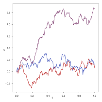
(a) Stochastic processes can be used to generate random functions: here we show three realisations from a Wiener process. The Wiener process is a continuous analogue of the random walk. Although usually presented as representing the movement of a particle, one can think of the path taken by the Wiener process as a function $y(t)$, and therefore of the Wiener process as generating a probability distribution over functions. The Wiener process is a GP, but GPs used in practice generate much smoother functions (see Figure 21 below).

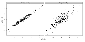
(b) We generated 200 realisations of the Wiener process, and plot their value at time $t=0.5$ against their value after either a small time lag ($\delta=0.02$), or a larger time lag ($\delta=0.2$). The smaller the time lag, the more these values are correlated. In general, this property is reflected in the covariance function of the GP.

Figure 19: The Wiener Process, a member of the family of Gaussian Processes.

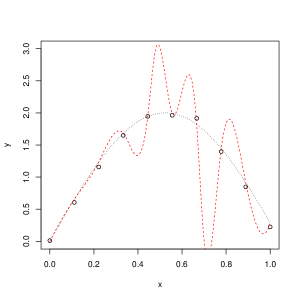
Figure 20: A non-parametric regression problem. We have measured some output $y$ for 10 different values of some covariate $x$. We plot these data as open circles. Our assumption is that $y=f(x)+\epsilon$, where $\epsilon$ is zero-mean noise. We wish to infer the underlying function $f$ from the data without assuming a parametric form for $f$. The two functions shown as dotted curves both have the same likelihood - they are equally close to the data. In most cases the function in red will be a far worse guess than the one in black. We need to inject that knowledge into our inference, and this can be done by imposing a prior on possible latent functions $f$. This can be done using a GP.

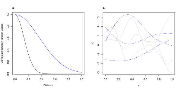
(a) GPs can be specified through their covariance function $k(x,x^{\prime})$. The covariance function expresses the following: if we were to measure $f$ at $x$ and $x^{\prime}$, how similar would we expect $f(x)$ and $f(x^{\prime})$ to be? The classical Gaussian or Matern families of covariance functions impose that expected similarity go down with the distance between $x$ and $x^{\prime}$. a. Two Gaussian covariance functions with different length-scales: correlation drops faster for one than the other (shorter length-scale). b. Samples from the corresponding GPs: we see that a shorter length-scale leads to less smooth functions.

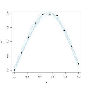
(b) Bayesian update of a Gaussian Process. We start with a prior distribution $p(f)$ over possible functions, then update the prior with data $\mathbf{y}$, to get a posterior $p(f|\mathbf{y})\propto p(\mathbf{y}|f)p(f)$. The posterior distribution is also a probability distribution, but relative to the prior it is concentrated over the functions that are likely given the data. On this Figure we show the data from Figure 20, along with functions sampled from the posterior distribution.

Figure 21: Gaussian Processes in the context of non-parametric regression. IPPs are distributions over point sets, GPs are distributions over functions. They can be used to specify a preference for “reasonable” functions.

5.3 Details on Inhomogeneous Poisson Processes

We give below some details on the likelihood function for inhomogeneous Poisson processes (IPPs), as well as the techniques we used for performing Bayesian inference.

5.3.1 The likelihood function of an IPP

An IPP is formally characterised as follows: given a spatial domain $\Omega$, e.g here $\Omega=[0,1]^{2}$, and an intensity function $\lambda:\,\Omega\rightarrow\mathbb{R}^{\text{+}}$ then an IPP is a probability distribution over finite subsets $S$ of $\Omega$ such that, for all sets $\mathcal{D}\in\Omega$,

$$\left|S\cap\mathcal{D}\right|\sim Poi\left(\int_{\mathcal{D}}\lambda\left(x\right)\mbox{d}x\right)$$ (9)

$\left|S\cap\mathcal{D}\right|$ is short-hand for the cardinal of $S\cap\mathcal{D}$, the number of points sampled from the process that fall in region $\mathcal{D}$. Note that in IPP, for disjoint subsets $\mathcal{D}_{1},\ldots,\mathcal{D}_{r}$ the distributions of $\left|S\cap\mathcal{D}_{1}\right|,\ldots,\left|S\cap\mathcal{D}_{r}\right|$ are independent.

For purposes of Bayesian inference, we need to be able to compute the likelihood, which is the probability of the sampled point set $S$ viewed as a function of the intensity function $\lambda\left(\centerdot\right)$. We will try to motivate and summarize the necessary concepts without a rigorous mathematical derivation, interested readers should consult Illian et al., (2008) for details.

We note first that the likelihood can be approximated by gridding the data: we divide $\Omega$ into a discrete set of regions $\Omega_{1},\ldots,\Omega_{r}$, and count how many points in $S$ fell in each of these regions. The likelihood function for the gridded data is given directly by Equation 9 along with the independence assumption: noting $k_{1},\ldots,k_{r}$ the bin counts we have

$$p\left(k_{1},\ldots,k_{r}|\lambda\right) = \prod_{j=1\ldots r}\frac{\left(\lambda_{j}\right)^{k_{j}}}{k_{j}!}\exp\left(-\lambda_{j}\right)$$ (10)

$$\lambda_{j} = \int_{\Omega_{j}}\lambda\left(x\right)\mbox{d}x$$

Also, since $\Omega_{1},\ldots,\Omega_{r}$ is a partition of $\Omega$, $\prod\exp\left(-\lambda_{j}\right)=\exp(-\sum\lambda_{j})=\exp\left(-\int_{\Omega}\lambda\left(x\right)\mbox{d}x\right)$.

As we make the grid finer and finer we should recover the true likelihood, because ultimately if the grid is fine enough for all instance and purposes we will have the true locations. As we increase the number of grid points $r$, and the area of each region $\Omega_{j}$ shrinks, two things will happen:

• the counts will be either 0 (in the vast majority of empty regions), or 1 (around the locations $s_{1},\ldots,s_{n}$ of the points in $S$).

• the integrals $\int_{\Omega_{j}}\lambda\left(x\right)\mbox{d}x$ will tend to $\lambda\left(x_{j}\right)\mbox{d}x$, with $x_{j}$ any point in region $\Omega_{j}$. In dimension 1, this corresponds to saying that the area under a curve can be approximated by height x length for small intervals.

Injecting this into Equation (10), in the limit we have:

$$p(S|\lambda\left(\cdot\right))=\frac{1}{n}\left\{\prod_{i=1}^{n}\lambda\left(s_{i}\right)\mbox{d}x\right\}\exp\left(-\int_{\Omega}\lambda\left(x\right)\mbox{d}x\right)$$ (11)

Since the factors $dx$ and $n^{-1}$ are independent of $\lambda$ we can neglect them in the likelihood function.

5.3.2 Conditioning on the number of datapoints, computing predictive distributions

The Poisson process has a remarkable property (Illian et al.,, 2008): conditional on sampling $n$ points from a Poisson process with intensity function $\lambda\left(x,y\right)$, these $n$ points are distributed independently with density

$$\bar{\lambda}\left(x,y\right)=\frac{\lambda\left(x,y\right)}{\int\lambda\left(x,y\right)\mbox{d}x\mbox{d}y}$$

Intuitively speaking, this means that if you know the point process produced 1 point, then this point is more likely to be where intensity is high.

This property is the direct analogue of its better known discrete variant: if $z_{1},z_{2},\ldots,z_{n}$ are independently Poisson distributed with mean $\lambda_{1},\ldots,\lambda_{n}$, then their joint distribution conditional on their sum $\sum z_{i}$ is multinomial with probabilities $\pi_{i}=\frac{\lambda_{i}}{\sum\lambda_{j}}$. Indeed, the continuous case can be seen as the limit case of the discrete case.

We bring up this point because it has an important consequence for prediction. If the task is to predict where the 100 next points are going to be, then the relevant predictive distribution is:

$$p(S|S\mbox{ has size }n)=\prod_{i=1}^{n}\frac{\lambda\left(x_{i},y_{i}\right)}{\int\lambda\left(x,y\right)\mbox{d}x\mbox{d}y}$$ (12)

where $S$ is a point set of size $n$, whose points have $x$ coordinates $x_{1},\ldots,x_{n}$ and $y$ coordinates $y_{1},\ldots,y_{n}$ . Equation 12 is the right density to use when evaluating the predictive abilities of the model with $n$ known (for example if one wants to compute the predictive deviance).

In the main text we had models of the form:

$$\log\lambda_{i}\left(x,y\right)=\eta_{i}\left(x,y\right)=\alpha_{i}+\beta_{i}m_{i}(x,y)$$

and we saw that when predicting data for a new image $j$ we do not know the values of $\alpha_{j}$ and $\beta_{j}$, and need to average over them. The good news is that when $n$ is known we need not worry about the intercept $\alpha_{j}$: all values of $\alpha_{j}$ lead to the same predictive distribution, because $\alpha_{j}$ disappears in the normalisation in Equation 12. Given a distribution $p(\beta)$ for possible slopes, the predictive distribution is given by:

$$p(S_{j}|S_{j}\mbox{ has size }n) = \int p(\beta_{j})\prod_{i=1}^{n}\frac{\exp\left(\beta_{j}m_{j}(x_{i},y_{i})\right)}{\int\exp\left(\beta_{j}m_{j}(x,y)\right)\mbox{d}x\mbox{d}y}\mbox{d}\beta_{j}$$

It is important to realise that the distribution above does not factorise over points, unlike (12) above. Computation requires numerical or Monte Carlo integration over $\beta$ (as far as we know).

5.4 Approximations to the likelihood function

One difficulty immediately arises when considering Equation (11): we require the integral$\int_{\Omega}\lambda\left(x\right)\mbox{d}x$. While not a problem when $\lambda\left(\cdot\right)$ has some convenient closed form, in the cases we are interested in $\lambda(x)=\exp\left(\eta\left(x\right)\right)$, with $\eta\left(\cdot\right)$ a GP sample. The integral is therefore not analytically tractable. A more fundamental difficulty is that the posterior distribution $p(\lambda\left(\cdot\right)|S)$ is over an infinite-dimensional space of functions - how are we to represent it?

All solutions use some form of discretisation. A classical solution is to use the approximate likelihood obtained by binning the data (Eq. 10), which is an ordinary Poisson count likelihood. The bin intensities $\lambda_{j}=\int_{\Omega_{j}}\lambda\left(x\right)\mbox{d}x$ are approximated by assuming that bin area is small relative to the variation in $\lambda\left(\cdot\right)$, so that:

$$\lambda_{j}=\lambda\left(x_{j}\right)\left|\Omega_{j}\right|$$

with $|\Omega_{j}|$ the area of bin $\Omega_{j}$ and $x_{j}$. The approximate likelihood then only depends on the value of $\lambda\left(\cdot\right)$ at bin centres, so that we can now represent the posterior as the finite-dimensional distribution $p(\lambda_{1}\ldots\lambda_{r}|S)$. In practice we target rather $p(\eta_{1}\ldots\eta_{r}|S)$, for which the prior distribution is given by (see

$$\eta(x_{1}),\ldots,\eta(x_{r})\sim\mathcal{N}\left(0,\mathbf{K}_{\theta}\right)$$

Here $\mathbf{K}_{\theta}$ is the covariance matrix corresponding to the covariance function $k_{\theta}\left(\cdot,\cdot\right)$, and $\theta$ represents hyperparameters (e.g., marginal variance and length-scale of the process).

A disadvantage of the binning approach is that fine gridding in 2D requires many, many bins, which means that good spatial resolution requires dealing with very large covariance (or precision) matrices, slowing down inference.

Another solution, due to Berman and Turner, (1992), uses again the values of $\eta\left(\cdot\right)$ sampled at $r$ grid points, but approximates directly the original likelihood (11). The troublesome integral $\int_{\Omega}\lambda\left(x\right)\mbox{d}x$ is dealt with using simple numerical quadrature:

$$\int_{\Omega}\lambda\left(x\right)\mbox{d}x\approx\sum w_{j}\exp\left(\eta\left(x_{j}\right)\right)$$

where the $w_{j}$’s are quadrature weights. The values $\lambda\left(s_{i}\right)$ at the sampled points are interpolated from the known values at the grid points:

$$\lambda\left(s_{i}\right)=\exp\left(\sum_{j=1\ldots r}a_{ij}\eta\left(x_{j}\right)\right)$$

the $a_{ij}$ are interpolation weights. Injecting into (11) we have the approximate log-likelihood function:

$$\mathcal{L}\left(\eta\right)=\sum_{i,j}a_{ij}\eta\left(x_{j}\right)-\sum w_{j}\exp\left(\eta\left(x_{j}\right)\right)$$ (13)

This log-likelihood function is compatible with the INLA framework for inference in latent Gaussian models (see Rue et al.,, 2009 and the website www.r-inla.org). The same log-likelihood function can be also be used in the classical maximum-likelihood framework. Approximate confidence intervals and p-values for coefficients can be obtained from nested model comparisons, or using resampling techniques (these techniques are explained in most statistics textbooks, including Wasserman,, 2003).

5.5 Relating patch statistics to point process theory

As noted above much of the previous work in the literature has focused on the statistics of image patches as a way of characterising the role of local image features in saliency. In this section we will show that these analyses can be related to point process modelling, leading to new insights. First, patch classification task approximates IPP models under certain assumptions. Second, the common practice of measuring performance by the area under the ROC curve can be grounded in point process assumptions. Third, the alternative procedure which consists in measuring performance by the proportion of fixations in the most salient region is in fact just a variant of the ROC procedure when seen in the point process context.

5.5.1 The patch classification problem as an approximate to point process modeling

We show here that patch classification can be interpreted as an approximation to point process modeling. Although we focus on the techniques used in the eye movement literature, our analysis is very close in spirit to that of Baddeley et al., (2010) on the spatial logistic regression methods used in Geographic Information Systems. Note that Baddeley et al., (2010) contains in addition many interesting results not detailed here and much more careful mathematical analysis.

Performing a classical patch statistics analysis involves collecting for a set of $n$ fixations $n$ “positive” image patches around the fixation locations and $n$ “negative” image patches around $n$ control locations, and comparing the contents of the patches. To avoid certain technical issues to do with varying intercepts (which we discuss later), we suppose that all fixations come from the same image. The usual practice is to compute some summary statistics on each patch, for example its luminance and contrast, and we note $\mathbf{v}(x,y)\in\mathbb{R}^{d}$ the value of those summary statistics at location $x,y$. We will see that $\mathbf{v}(x,y)$ plays the role of spatial covariates in point process models. We assume that the $n$ control locations are drawn uniformly from the image.

The next step in the classical analysis is to compare the conditional distributions of $\mathbf{v}$ for positive and negative patches, which we will denote $p(\mathbf{v}|s=1)$ and $p(\mathbf{v}|s=0)$. If these conditional distributions are different, than they afford us some way to tell between selected and non-selected locations based on the contents of the patch. Equivalently, $p\left(s|\mathbf{v}\right)$, the probability of the patch label given the covariates, is different from the base rate of 50% for certain values of $\mathbf{v}$. Patch classification is concerned with modelling $p(s|\mathbf{v})$, a classical machine learning problem that can be tackled via logistic regression or a support vector machine, as in Kienzle et al., (2009).

Under certain conditions, statistical analysis of the patch classification problem can be related to point process modelling. Patch classification can be related to spatial logistic regression, which in turn can be shown to be an approximation of the IPP model (Baddeley et al.,, 2010). We give here a simple proof sketch that deliberately ignores certain technical difficulties associated with the smoothness (or lack thereof) of $\mathbf{v}\left(x,y\right)$.

In spatial logistic regression, a set of fixations is turned into binary data by dividing the domain into a large set of pixels $a_{1}\ldots a_{r}$ and defining a binary vector $z_{1}\ldots z_{r}$ such that $z_{i}=1$ if pixel $a_{i}$ contains a fixation and $z_{i}=0$ otherwise. The second step is to regress these binary data onto the spatial covariates using logistic regression, which implies the following statistical model:

$$p\left(\mathbf{z}|{\bf\beta}\right) =\prod_{i=1}^{r}\Lambda\left({\bf\beta}^{t}\mathbf{v}_{i}+\beta_{0}\right)^{z_{i}}\left(1-\Lambda\left({\bf\beta}^{t}\mathbf{v}_{i}+\beta_{0}\right)\right)^{1-z_{i}}$$ (14)

$$\Lambda\left(\eta\right) =\frac{1}{1+e^{-\eta}}$$ (15)

Equation 15 is just the logistic function, and the value $\mathbf{v}_{i}$ of the covariates at the $i-$th pixel can be either the average value over the pixel or the value at the center of the pixel. By the Poisson limit theorem, the independent Bernoulli likelihood of Equation 14 becomes that of a Poisson process as pixel size tends to 0. In this limit the probability of observing any individual $z_{i}=1$ will be quite small, so that $\eta_{i}={\bf\beta}^{t}\mathbf{v}_{i}+\beta_{0}$ will be well under 0 around the peak of the likelihood. For small values of $\eta$, $\Lambda\left(\eta\right)\approx\exp\left(\eta\right)$, so that:

$$p\left(\mathbf{z}|{\bf\beta}\right)\approx\prod_{i=1}^{r}\exp\left({\bf\beta}^{t}\mathbf{v}_{i}+\beta_{0}\right)^{z_{i}}\left(1-\exp\left({\bf\beta}^{t}\mathbf{v}_{i}+\beta_{0}\right)\right)^{1-z_{i}}$$

We take the log of $p\left(\mathbf{z}|{\bf\beta}\right)$ and split the indices of the pixels according to the value of $z_{i}$: we note $\mathcal{I}^{+}$ the set of selected pixels (pixels such that $z_{i}=1$), $\mathcal{I}^{-}$ its complement. This yields:

$$\log\,p\left(\mathbf{z}|{\bf\beta}\right)\approx\sum_{\mathcal{I}^{+}}\left\{{\bf\beta}^{t}\mathbf{v}_{i}+\beta_{0}\right\}+\sum_{\mathcal{I}^{-}}\left\{\log\left(1-\exp\left({\bf\beta}^{t}\mathbf{v}_{i}+\beta_{0}\right)\right)\right\}$$

We make use again of the fact that Bernoulli probabilities will be small, which implies that $1-\exp\left({\bf\beta}^{t}\mathbf{v}_{i}+\beta_{0}\right)$ will be close to 1. Since $\log\left(x\right)\approx x-1$ for $x\approx 1$, the approximation can be further simplified to:

$$\log\,p\left(\mathbf{z}|{\bf\beta}\right)\approx\sum_{\mathcal{I}^{+}}\left\{{\bf\beta}^{t}\mathbf{v}_{i}+\beta_{0}\right\}-\sum_{\mathcal{I}^{-}}\exp\left({\bf\beta}^{t}\mathbf{v}_{i}+\beta_{0}\right)$$

If the pixel grid is fine enough the second part of the sum will cover almost every point, and will therefore be proportional to the integral of ${\bf\beta}^{t}\mathbf{v}\left(x,y\right)+\beta_{0}$ over the domain. This shows that the approximate likelihood given in Equation (14) tends to the likelihood of an IPP (Eq. 11) with log intensity function $\log\lambda\left(x,y\right)={\bf\beta}^{t}\mathbf{v}\left(x,y\right)+\beta_{0}$, which is exactly the kind used in this manuscript.

This establishes the small-pixel equivalence of spatial logistic regression and IPP modeling. It remains to show that spatial logistic regression and patch classification are in some cases equivalent.

In the case described above, one has data for one image only, collects $n$ patches at random as examples of non-fixated locations, and then performs logistic regression on the patch labels based on the patch statistics $\mathbf{v}_{i}$. This is essentially the same practice often used in spatial logistic regression, where people simply throw out some of the (overabundant) negative examples at random. Throwing out negative examples leads to a loss in efficiency, as shown in Baddeley et al., (2010) . It is interesting to note that under the assumption that fixations are generated from a IPP with intensity $\lambda\left(x,y\right)={\bf\beta}^{t}\mathbf{v}\left(x,y\right)+\beta_{0}$, giving us $n$ positive examples, and assuming that the $n$ negative examples are generated uniformly, the logistic likelihood becomes exact (this is a variant of lemma 12 in Baddeley et al.,, 2010). The odds-ratio that a point at location $x,y$ was one of the original fixations is simply:

$$\log\,\frac{p(z=1|x,y)}{p(z=0|x,y)}=\log\,\frac{\lambda\left(x,y\right)}{A^{-1}}={\bf\beta}^{t}\mathbf{v}\left(x,y\right)+\beta_{0}+\log\left(A\right)$$ (16)

Here $A$ is the total area of the domain. Equation 16 shows in another way the close relationship between patch classification and spatial point process models: patch classification using logistic regression is a correct (but inefficient) model under IPP assumptions.

In actual practice patch classification involves a) combining patches from multiple images and b) possibly different techniques for classification than logistic regression. The first issue may be problematic, since as we have shown above the coefficients relating covariates to intensity, and certainly intercept values, may vary substantially from one image to another. This can be fixed by changing the covariate matrix appropriately in the logistic regression.

The second issue is that, rather than logistic regression, other classification methods may be used : does the point process interpretation remain valid? If one uses support vector machines, then the answer is yes, at least in the limit of large datasets (SVM and logistic regression are asymptotically equivalent, see Steinwart,, 2005): the coefficients will differ only in magnitude. The same holds for probit, complementary log-log or even least-squares regression: the correct coefficients will be asymptotically recovered up to a scaling factor. In actual practice, the difference between classification methods is often small and all of them may equally be thought of as approximating point process modeling.

5.5.2 ROC performance measures, area counts, and minimum volume sets

Many authors have used the area under the ROC curve as a performance measure for patch classification. Another technique, used for example in Torralba et al., (2006), is to take the image region with the 20% most salient pixels and count the proportion of fixations that occured in this region (a proportion over 20% is counted as above-chance performance). We show below that the two procedures are related to each other and to point process models. The notion of minimum volume regions will be needed repeatedly in the development below, and we therefore begin with some background material.

Minimum-volume sets

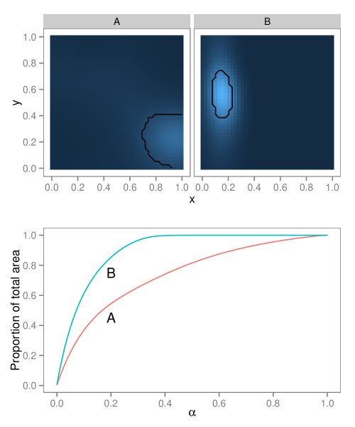
Figure 22: Minimum volume sets. We show in the upper panel two density functions (A) and (B) along with minimal volume sets with $\alpha=0.8$: these are the smallest areas containing 80% of the probability, and correspond to contours of the density (see text). The $\alpha=0.8$ area is much larger in A than in B, which reflects higher uncertainty. In the lower panel, the area of the minimal volume set of level $\alpha$ is represented as a function of the confidence level $\alpha$. The integral of this function is shown in the text to equal optimal ROC performance in the patch classification problem, and reflects the underlying uncertainty in the point process.

A minimum-volume set with confidence level $\alpha$ is the smallest region that will contain a point with probability at least $\alpha$ (it extends the notion of a confidence interval to arbitrary domains, see Fig. 22). Formally, given a probability density $\pi(s)$ over some domain, the minimum volume set $F_{\alpha}$ is such that:

$$F_{\alpha} =\underset{F\in\mathcal{M}\left(\Omega\right)}{\mbox{argmin}}\mbox{Vol}\left(F\right)$$ (17)

subject to $$\int_{F}\pi\geq\alpha$$

where the minimisation is over all measurable subsets of the domain $\Omega$ and $\mbox{Vol}\left(F\right)=\int_{F}1$ is the total volume of set $F$. Intuitively speaking, the smaller the minimum-volume sets of $\pi$, the less uncertainty there is: if 99% of the probability is concentrated in just 20% of the domain, then $\pi$ is in some sense 5 times more concentrated than the uniform distribution over $\Omega$. In the case of Gaussian distributions the minimum volume sets are ellipses, but for arbitrary densities they may have arbitrary shapes. In Nuñez Garcia et al., (2003) it is shown that the family of minimum volume sets of $\pi$ is equal to the family of contour sets of $\pi$: that is, every set $F_{\alpha}$ is equal to a set $\left\{s\in\Omega|\pi\left(s\right)\geq\pi_{0}\right\}$ for some value $\pi_{0}$ that depends on $\alpha$. We can therefore measure the amount of uncertainty in a distribution by looking at the volume of its contour sets, a notion which will arise below when we look at optimal ROC performance.

ROC measures

In ROC-based performance measures, the output of a saliency model $m(x,y)$ is used to classify patches as fixated or not, and performance classification is measured using the area of under the ROC curve. The ROC curve is computed by varying a criterion $\xi$ and counting the rate of False Alarms and Hits that result from classifying a patch as fixated. In this section we relate this performance measure to point process theory and show that:

1. If non-fixated patches are sampled from a homogeneous PP, and fixated patches from a IPP with intensity $\lambda\left(x,y\right)$, then the optimal saliency model in the sense of the AUC metric is $\lambda(x,y)$ (or any monotonic transformation thereof). In this case the AUC metric measures the precision of the IPP, i.e. how different from the uniform intensity function $\lambda\left(x,y\right)$ is.

2. If non-fixated patches are not sampled from a uniform distribution, but from some other PP with intensity $\varphi\left(x,y\right)$, then the optimal saliency model in the sense of the AUC metric is no longer $\lambda\left(x,y\right)$ but $\frac{\lambda\left(x,y\right)}{\varphi\left(x,y\right)}$. In other words, a saliency model could correctly predict fixation locations but perform sub-optimally according to the AUC metric if non-fixated locations are sampled from a non-uniform distribution (for example when non-fixated locations are taken from other pictures).

3. Since AUC performance is invariant to monotonic transformations of $m(x,y)$, it says nothing about how intensity scales with $m(x,y)$.

In the following we will simplify notation by noting spatial locations as $s=(x,y)$, and change our notation for functions accordingly ($m(s),\lambda(s)$, etc.). We assume that fixated patches are drawn from a PP with intensity $\lambda(s)$ and non-fixated patches from a PP with intensity $\varphi\left(s\right)$. In ROC analysis locations are examined independently from one another, so that all that matters are the normalised intensity functions (probability densities for single points, see Section 5.3.2). Without loss of generality we assume that $\lambda$ and $\varphi$ integrate to 1 over the domain.

By analogy with psychophysics we define the task of deciding whether a single, random patch $s$ was drawn from $\lambda$ (the fixated distribution) or $\varphi$ (the non-fixated distribution) as the Yes/No task. Correspondingly, the 2AFC task is the following: two patches $s_{1},s_{2}$ are sampled random, one from $\lambda$ and one from $\varphi$, and one must guess which of the two patches came from $\lambda$. The Y/N task is performed by comparing the “saliency” of the patch $m(s)$ to a criterion $\xi$. The 2AFC task is performed by comparing the relative saliency of $s_{1}$ and $s_{2}$: if $m(s_{1})>m(s_{2})$ the decision is that $s_{1}$ is the fixated location.

We will use the fact that the area under the ROC curve is equal to 2AFC performance (Green and Swets,, 1966). 2AFC performance can be computed as follows: we note $O=\left(1,0\right)$ the event corresponding to $s_{1}\sim\lambda$ and $s_{2}\sim\varphi$. The probability of a correct decision under the event $O=(1,0)$ is:

$$p_{c}=\int_{\Omega}\lambda(s_{1})\left\{\int_{\Omega}\varphi\left(s_{2}\right)\mathbb{I}\left(m\left(s_{1}\right)>m(s_{2})\right)\mbox{d}s_{2}\right\}\mbox{d}s_{1}$$ (18)

where $\mathbb{I}\left(m\left(s_{1}\right)>m(s_{2})\right)$ is the indicator function of the event that $s_{1}$ has higher saliency than $s_{2}$ (according to $m$). Note that the $O=\left(0,1\right)$ event is exactly symmetrical, so that we do not need to consider both.

We first consider the case where non-fixated locations are drawn uniformly ($\varphi\left(s\right)=V^{-1}$, where $V$ is the area or volume of the observation window), and ask what the optimal saliency map $m$ is - in the sense of giving maximal 2AFC performance and therefore maximal AUC. 2AFC can be viewed as a categorisation task over a space of stimulus pairs, where the two categories are $O=(1,0)$ and $O=(0,1)$ in our notation. The so-called “Bayes rule” is the optimal rule for categorisation (Duda et al.,, 2000), and in our case it takes the following form: answer $O=(1,0)$ if $p\left(O=(1,0)|s_{1},s_{2})\right)>p\left(O=(0,1)|s_{1},s_{2}\right)$. The prior probability $p\left(O=(0,1)|s_{1},s_{2}\right)$ is $1/2$, so the decision rule only depends on the likelihood ratio:

$$\frac{p\left(s_{1},s_{2}|O=(1,0)\right)}{p\left(s_{1},s_{2}|O=(0,1)\right)}=\frac{\lambda\left(s_{1}\right)\varphi\left(s_{2}\right)}{\lambda\left(s_{2}\right)\varphi\left(s_{1}\right)}=\frac{\lambda\left(s_{1}\right)}{\lambda\left(s_{2}\right)}$$ (19)

The optimal decision rule consist in comparing $\lambda(s_{2})$ to $\lambda\left(s_{1}\right)$, which is equivalent to using $\lambda$ as a saliency map (or any other monotonic transformation of $\lambda$). The probability of a correct decision (18) is then:

$$p_{c}=\int_{\Omega}\lambda(s_{1})\left\{V^{-1}\int_{\Omega}\mathbb{I}\left(\lambda\left(s_{1}\right)\geq\lambda(s_{2})\right)\mbox{d}s_{2}\right\}\mbox{d}s_{1}$$ (20)

The inner integral $\int_{\Omega}\mathbb{I}\left(\lambda\left(s_{1}\right)\geq\lambda(s_{2})\right)\mbox{d}s_{2}$ corresponds to the total volume of the set of all locations with lower density than the value at $s_{1}$: a contour set of $\lambda$, which as we have seen is also a minimum volume set. This observation leads to another of expressing the integral in (20): intuitively, each location $s_{1}$ will be on the boundary of a minimum volume set $F_{\alpha}$, for some value of $\alpha$, and the inner integral will correspond to the volume of that set. We re-express the integral by grouping together all values of $s_{1}$ that lead to the same set $F_{\alpha}$, and hence the same value of the inner integral: these are the set of values $s_{1}$ that fall along a density contour $\lambda\left(s_{1}\right)=\lambda_{\alpha}$. Suppose that we generate a random value of $s_{1}$ and note the $\alpha$ value of the contour set $s_{1}$ falls on: call $a$ this random variable. By definition the event $s_{1}\in F_{\alpha}$ happens with probability $\alpha$, so that $p(a\leq\alpha)=\alpha$, and therefore $a$ has a uniform distribution over $[0,1]$ (it is in fact a p-value). We can express Equation (20) as an expectation over $a$:

$$p_{c}=\int_{0}^{1}p(a=\alpha)\left(1-V\left(\alpha\right)\right)\mbox{d}a=1-\int_{0}^{1}V\left(\alpha\right)\mbox{d}\alpha$$ (21)

Here $V\left(\alpha\right)$ is the relative volume of the minimum-volume set with confidence level $\alpha.$ $V(0.9)=0.2$ means that, for a location $s$ sampled from $\lambda$, the smallest region of space we can find that includes 90% of the observations takes up just 20% of the observation window. For a uniform distribution $V\left(\alpha\right)=\alpha$. Whatever the density $\lambda$, $V\left(0\right)=0$, and if small regions include most of the probability mass we are going to see a slow increase in $V\left(\alpha\right)$ as $\alpha$ rises. This will lead in turn to a low value for the integral $\int_{0}^{1}V\left(\alpha\right)\mbox{d}\alpha$. Having small regions that contain most of the probability mass is the same as having a concentrated or precise point process, and therefore Equation (21) shows that under the optimal decision rule the AUC value measures the precision of the point process.

We now turn to the case where non-fixated locations are not taken from the uniform distribution: for example, when those locations are randomly drawn from fixations observed on other pictures. The optimal rule is again Bayes’ rule, Equation 19, which is equivalent to using $m(s)=\lambda(s)/\varphi\left(s\right)$ as a saliency map. Under an assumption of center bias this may artificially inflate the AUC value of saliency maps which have low values around the center. This problem can be remedied by computing an estimate of the intensity $\varphi$ and using $m(s)/\varphi(s)$ (or more conveniently $\log m(s)-\log\varphi\left(s\right))$ instead of $m(s)$ when computing AUC scores.

Area counts

In area counts the goal is to have a small region that contains as many fixations as possible. Given a discrete saliency map, we can build a region that contains the 20% most salient pixels, and count the number of fixations that occured there. In this section we show that if fixations come from a point process with intensity $\lambda$, the optimal saliency map is again $\lambda$ (again, up to arbitrary monotonic transformations). In that context, we show further that if we remove the arbitrariness of setting a criterion at 20%, and integrate over criterion position, we recover exactly the AUC performance measure - the two become equivalent.

Let us define the following optimisation problem: given a probability density $\pi$, we seek a measurable set $G$ such that

$$G_{q} =\underset{F\in\mathcal{M}\left(\Omega\right)}{\mbox{argmax}}\int_{G}\pi$$ (22)

s.t $$V\left(G\right)=q$$

that is, among all measurable subsets of $\Omega$ of relative volume $q$, we seek the one that has maximum probability under $\pi$. These maximum-probability sets and the minimum-volume-sets defined above are related: indeed the optimisation problems that define them (17 and 22) are dual. This follows from writing down the Lagrangian of 22:

$$\mathcal{L}\left(G,\eta\right)=\int_{G}\pi+\eta\left(V\left(G\right)-q\right)$$

which is equivalent to that of (17) for some value of $\eta$. This result implies that the family of solutions of the two problems are the same: a maximum-probability set for some volume $q$ is a minimum-volume set for some confidence level $\alpha$. Since we know that the family of contours sets is the family of solutions of the minimum-volume problem, it follows that it is also the family of solutions of the maximum-probability problem.

In turn, this implies that if fixations come from an IPP with intensity $\lambda$, the optimal saliency map according to the area count metric must have the same top 20% values in the same locations as $\lambda$. To remove the arbitrariness associated with the criterion, we measure the total probability in $G_{q}$ for each value of $q$ between 0 and 1 and integrate:

$$A_{c}=\int_{0}^{1}\left(\int_{G_{q}}\lambda\left(s\right)\mbox{d}s\right)\mbox{d}q=\int_{0}^{1}\mbox{Prob}\left(q\right)\mbox{d}q$$

The integrand $\mbox{Prob}\left(q\right)$ measures the probability contained within the maximum-probability set of size $q$: because of the equivalence of maximum-probability and minimum-coverage sets, $\mbox{Prob}(q)$ is the inverse of the function $V\left(\alpha\right)$, which measured the relative size of the minimum-volume set with confidence level $\alpha$. Therefore $A_{c}=1-\int_{0}^{1}V\left(\alpha\right)\mbox{d}\alpha$, which is exactly the optimal AUC performance under uniform samples, as shown in the previous section. Area counts and ROC performance are therefore tightly related.

References

- Baddeley et al., (2010) Baddeley, A., Berman, M., Fisher, N. I., Hardegen, A., Milne, R. K., Schuhmacher, D., Shah, R., and Turner, R. (2010). Spatial logistic regression and change-of-support in poisson point processes. Electronic Journal of Statistics, 4(0):1151–1201.
- Baddeley et al., (2005) Baddeley, A., Turner, R., Møller, J., and Hazelton, M. (2005). Residual analysis for spatial point processes (with discussion). Journal of the Royal Statistical Society: Series B (Statistical Methodology), 67(5):617–666.
- Berman and Turner, (1992) Berman, M. and Turner, T. R. (1992). Approximating point process likelihoods with GLIM. Applied Statistics, 41(1):31–38.
- Bishop, (2007) Bishop, C. M. (2007). Pattern Recognition and Machine Learning (Information Science and Statistics). Springer, 1st ed. 2006. corr. 2nd printing edition.
- Borji and Itti, (2013) Borji, A. and Itti, L. (2013). State-of-the-art in visual attention modeling. IEEE Transactions On Pattern Analysis And Machine Intelligence, 35(1):185–207.
- Bruce and Tsotsos, (2009) Bruce, N. D. and Tsotsos, J. K. (2009). Saliency, attention, and visual search: an information theoretic approach. Journal of vision, 9(3).
- Cerf et al., (2008) Cerf, M., Harel, J., Einhäuser, W., and Koch, C. (2008). Predicting human gaze using low-level saliency combined with face detection. Advances in neural information processing systems, 20.
- Ciuffreda and Tannen, (1995) Ciuffreda, K. J. and Tannen, B. (1995). Eye movement basics for the clinician. Mosby, St Louis.
- Dayan and Abbott, (2001) Dayan, P. and Abbott, L. F. (2001). Theoretical Neuroscience: Computational and Mathematical Modeling of Neural Systems. The MIT Press, 1st edition.
- Deubel and Schneider, (1996) Deubel, H. and Schneider, W. X. (1996). Saccade target selection and object recognition: Evidence for a common attentional mechanism. Vision Research, 36:1827–1837.
- Diggle, (2002) Diggle, P. J. (2002). Statistical Analysis of Spatial Point Patterns. Hodder Education Publishers, 2 edition.
- Duda et al., (2000) Duda, R. O., Hart, P. E., and Stork, D. G. (2000). Pattern Classification (2nd Edition). Wiley-Interscience, 2 edition.
- Ehinger et al., (2009) Ehinger, K. A., Hidalgo-Sotelo, B., Torralba, A., and Oliva, A. (2009). Modeling search for people in 900 scenes: A combined source model of eye guidance. Visual cognition, 17(6-7):945–978.
- Einhäuser et al., (2008) Einhäuser, W., Spain, M., and Perona, P. (2008). Objects predict fixations better than early saliency. Journal of Vision, 8(14).
- Engbert and Mergenthaler, (2006) Engbert, R. and Mergenthaler, K. (2006). Microsaccades are triggered by low retinal image slip. Proceedings of the National Academy of Sciences, 103(18):7192–7197.
- Engbert et al., (2005) Engbert, R., Nuthmann, A., Richter, E. M., and Kliegl, R. (2005). SWIFT: A dynamical model of saccade generation during reading. Psychological Review, 112(4):777–813.
- Fecteau and Munoz, (2006) Fecteau, J. H. and Munoz, D. P. (2006). Salience, relevance, and firing: a priority map for target selection. Trends in cognitive sciences, 10(8):382–390.
- Fei-Fei et al., (2007) Fei-Fei, L., Iyer, A., Koch, C., and Perona, P. (2007). What do we perceive in a glance of a real-world scene? Journal of vision, 7(1):1–29.
- Fründ et al., (2011) Fründ, I., Haenel, N. V., and Wichmann, F. A. (2011). Inference for psychometric functions in the presence of nonstationary behavior. Journal of Vision, 11(6).
- Gelman and Hill, (2006) Gelman, A. and Hill, J. (2006). Data Analysis Using Regression and Multilevel/Hierarchical Models. Cambridge University Press.
- Green and Swets, (1966) Green, D. M. and Swets, J. A. (1966). Signal Detection Theory and Psychophysics. John Wiley and Sons.
- Haran and Tierney, (2012) Haran, M. and Tierney, L. (2012). On automating markov chain monte carlo for a class of spatial models.
- Hastie et al., (2003) Hastie, T., Tibshirani, R., and Friedman, J. H. (2003). The Elements of Statistical Learning. Springer, corrected edition.
- Henderson, (2003) Henderson, J. M. (2003). Human gaze control during real-world scene perception. Trends in cognitive sciences, 7(11):498–504.
- Henderson, (2011) Henderson, J. M. (2011). Eye movements and scene perception. In Liversedge, S. P., Gilchrist, I. D., and Everling, S., editors, The Oxford Handbook of Eye Movements, pages 593–606. Oxford University Press, Oxford, UK.
- Henderson et al., (2007) Henderson, J. M., Brockmole, J., Castelhano, M., and Mack, M. (2007). Visual saliency does not account for eye movements during search in real-world scenes, pages 537–562. Elsevier.
- Henderson and Ferreira, (2004) Henderson, J. M. and Ferreira, F. (2004). Scene perception for psycholinguists. In Henderson, J. M. and Ferreira, F., editors, The interface of language, vision, & action, pages 1–58. Psychology Press.
- Illian et al., (2009) Illian, J., Møller, J., and Waagepetersen, R. (2009). Hierarchical spatial point process analysis for a plant community with high biodiversity. Environmental and Ecological Statistics, 16(3):389–405.
- Illian et al., (2008) Illian, J., Penttinen, A., Stoyan, H., and Stoyan, D. (2008). Statistical Analysis and Modelling of Spatial Point Patterns (Statistics in Practice). Wiley-Interscience, 1 edition.
- Itti, (2004) Itti, L. (2004). Automatic foveation for video compression using a neurobiological model of visual attention. Image Processing, IEEE Transactions on, 13(10):1304–1318.
- Itti and Koch, (2001) Itti, L. and Koch, C. (2001). Computational modelling of visual attention. Nature reviews. Neuroscience, 2(3):194–203.
- Judd et al., (2009) Judd, T., Ehinger, K., Durand, F., and Torralba, A. (2009). Learning to predict where humans look. In Computer Vision, 2009 IEEE 12th international conference on, pages 2106–2113. IEEE.
- Kanan et al., (2009) Kanan, C., Tong, M. H., Zhang, L., and Cottrell, G. W. (2009). SUN: Top-down saliency using natural statistics. Visual cognition, 17(6-7):979–1003.
- Kaspar and König, (2011) Kaspar, K. and König, P. (2011). Viewing behavior and the impact of low-level image properties across repeated presentations of complex scenes. Journal of Vision, 11(13).
- Kienzle et al., (2009) Kienzle, W., Franz, M. O., Schölkopf, B., and Wichmann, F. A. (2009). Center-surround patterns emerge as optimal predictors for human saccade targets. Journal of vision, 9(5).
- Kliegl et al., (2006) Kliegl, R., Nuthmann, A., and Engbert, R. (2006). Tracking the mind during reading: the influence of past, present, and future words on fixation durations. Journal of experimental psychology. General, 135(1):12–35.
- Koch and Ullman, (1985) Koch, C. and Ullman, S. (1985). Shifts in selective visual attention: towards the underlying neural circuitry. Human neurobiology, 4(4):219–227.
- Krieger et al., (2000) Krieger, G., Rentschler, I., Hauske, G., Schill, K., and Zetzsche, C. (2000). Object and scene analysis by saccadic eye-movements: an investigation with higher-order statistics. Spatial vision, 13(2-3):201–214.
- Kruschke, (2010) Kruschke, J. K. (2010). Doing Bayesian Data Analysis: A Tutorial with R and BUGS. Academic Press, 1 edition.
- Land and Tatler, (2009) Land, M. F. and Tatler, B. W. (2009). Looking and Acting: Vision and Eye Movements in Natural Behaviour. Oxford University Press: New York.
- Lewis and Shedler, (1979) Lewis, P. A. W. and Shedler, G. S. (1979). Simulation of nonhomogeneous poisson processes by thinning. Naval Research Logistics, 26(3):403–413.
- Mannan et al., (1996) Mannan, S. K., Ruddock, K. H., and Wooding, D. S. (1996). The relationship between the locations of spatial features and those of fixations made during visual examination of briefly presented images. Spatial Vision, pages 165–188.
- Matin, (1974) Matin, E. (1974). Saccadic suppression: A review and an analysis. Psychological Bulletin, 81(12):899–917.
- McCullagh and Nelder, (1989) McCullagh, P. and Nelder, J. A. (1989). Generalized Linear Models, Second Edition (Chapman & Hall/CRC Monographs on Statistics & Applied Probability). Chapman and Hall/CRC, 2 edition.
- Mergenthaler and Engbert, (2010) Mergenthaler, K. and Engbert, R. (2010). Microsaccades are different from saccades in scene perception. Experimental brain research. Experimentelle Hirnforschung. Expérimentation cérébrale, 203(4):753–757.
- Nuñez Garcia et al., (2003) Nuñez Garcia, J., Kutalik, Z., Cho, K.-H., and Wolkenhauer, O. (2003). Level sets and minimum volume sets of probability density functions. International Journal of Approximate Reasoning, 34(1):25–47.
- Nuthmann and Henderson, (2010) Nuthmann, A. and Henderson, J. M. (2010). Object-based attentional selection in scene viewing. Journal of vision, 10(8).
- Nuthmann et al., (2010) Nuthmann, A., Smith, T. J., Engbert, R., and Henderson, J. M. (2010). CRISP: A computational model of fixation durations in scene viewing. Psychological Review, 117(2):382–405.
- Park et al., (2011) Park, M., Horwitz, G., and Pillow, J. W. (2011). Active learning of neural response functions with gaussian processes. In Shawe-Taylor, J., Zemel, R., Bartlett, P., Pereira, F., and Weinberger, K., editors, Advances in Neural Information Processing Systems 24, pages 2043–2051.
- Parkhurst and Niebur, (2003) Parkhurst, D. J. and Niebur, E. (2003). Scene content selected by active vision. Spatial vision, 16(2):125–154.
- Pitt et al., (2002) Pitt, M. A., Myung, I. J. J., and Zhang, S. (2002). Toward a method of selecting among computational models of cognition. Psychological review, 109(3):472–491.
- Rajashekar et al., (2007) Rajashekar, U., van der Linde, I., Bovik, A. C., and Cormack, L. K. (2007). Foveated analysis of image features at fixations. Vision research, 47(25):3160–3172.
- Rasmussen and Williams, (2005) Rasmussen, C. E. and Williams, C. K. I. (2005). Gaussian Processes for Machine Learning (Adaptive Computation and Machine Learning series). The MIT Press.
- Rayner, (2009) Rayner, K. (2009). Eye movements and attention in reading, scene perception, and visual search. The Quarterly Journal of Experimental Psychology.