Invasion fronts with variable motility: phenotype selection, spatial sorting and wave acceleration

Abstract

Invasion fronts in ecology are well studied but very few mathematical results concern the case with variable motility (possibly due to mutations). Based on an apparently simple reaction-diffusion equation, we explain the observed phenomena of front acceleration (when the motility is unbounded) as well as other quantitative results, such as the selection of the most motile individuals (when the motility is bounded). The key argument for the construction and analysis of traveling fronts is the derivation of the dispersion relation linking the speed of the wave and the spatial decay. When the motility is unbounded we show that the position of the front scales as $t^{3/2}$. When the mutation rate is low we show that the canonical equation for the dynamics of the fittest trait should be stated as a PDE in our context. It turns out to be a type of Burgers equation with source term.

Résumé Fronts d’invasion avec motilité variable: répartition des phénotypes et accélération de l’onde. Les fronts d’invasion en écologie ont été largement étudiés. Cependant peu de résultats mathématiques existent pour le cas d’un coefficient de motilité variable (à cause des mutations). A partir d’un modèle minimal de réaction-diffusion, nous expliquons le phénomène observé d’accélération du front (lorsque la motilité n’est pas bornée), et nous démontrons l’existence d’ondes progressives ainsi que la sélection des individus les plus motiles (lorsque la motilité est bornée). Le point clé pour la construction des fronts est la relation de dispersion qui relie la vitesse de l’onde avec la décroissance en espace. Lorsque la motilité n’est pas bornée nous montrons que la position du front suit une loi d’échelle en $t^{3/2}$. Lorsque le taux de mutation est faible, nous montrons que, dans notre contexte, l’équation canonique pour la dynamique du meilleur trait est une EDP. C’est une équation de type Burgers avec terme source.

, , , , , ,

Received *****; accepted after revision +++++
Presented by £££££

Version française abrégée

Dans cette note nous étudions un modèle simple décrivant des fronts invasifs en écologie, pour lesquels la mobilité des individus est sujette à variations. Le modèle, issu de [1], est le suivant,

$$\begin{cases}\partial_{t}n(t,x,\theta)=\theta\partial^{2}_{xx}n(t,x,\theta)+rn(t,x,\theta)\left(1-\rho(t,x)\right)+\alpha\partial^{2}_{\theta\theta}n(t,x,\theta)\,,\quad x\in(-\infty,+\infty),\,\theta>0\,,\\ \rho(t,x)=\int n(t,x,\theta)\,d\theta\,,\qquad n(t,-\infty,\theta)=\overline{N}(\theta)\,,\qquad n(t,+\infty,\theta)=0\,.\end{cases}$$ (1)

Les conditions aux limites sont complétées ci-dessous. Nous étudions la dynamique de cette équation sous différents régimes. Dans un premier temps nous étudions le problème de propagation de front à vitesse constante. Cela circonscrit l’espace des traits $\theta\in(0,\Theta)$, qui doit être borné $\Theta<+\infty$. Nous démontrons que la situation est similaire au cas de l’équation de Fisher-KPP. Il existe une vitesse minimale $c^{*}$ de propagation des ondes de réaction-diffusion (Théorème 1). La relation de dispersion, analogue à celle de Fisher-KPP (un trinôme du second degré en l’occurrence) est donnée via la résolution d’un problème spectral. On lit sur la distribution des phénotypes (le vecteur propre) que les fortes motilités sont favorisées, conclusion opposée au cas des domaines bornés en espace [2]. Ce même problème spectral intervient lorsqu’on étudie la propagation du front en régime asymptotique hyperbolique $(t,x)\to(t/\varepsilon,x/\varepsilon)$ dans la limite WKB de l’optique géométrique, en suivant l’ansatz $n^{\varepsilon}(t,x,\theta)=\exp(u^{\varepsilon}(t,x)/\varepsilon)N^{\varepsilon}(t,x,\theta)$.

Dans un second temps, nous considérons un espace des traits non borné, $\Theta=+\infty$. Dans ce cas le front accélère sans cesse et nous montrons heuristiquement que la loi de propagation du front est naturellement $\langle x\rangle\sim\left(\alpha^{1/4}r^{3/4}\right)t^{3/2}$. Nous exhibons une solution particulière qui confirme cette heuristique (Proposition 2).

Dans un troisième temps, nous étudions le régime de mutations rares, et nous écrivons une équation canonique pour l’évolution du trait sélectionné localement à l’avant du front en régime asymptotique. La dérivation formelle de cette équation conduit à une équation de transport de type Burgers, avec terme source (Proposition 3). La partie transport est dûe à la progression du front qui ”transporte” les individus et donc le trait sélectionné localement. Le terme source est dû à la pression de sélection qui tend à faire augmenter la valeur du trait sélectionné localement.

Introduction

Recently, several works have addressed the issue of front invasion in ecology, where the motility of individuals is subject to variability [3, 4]. It has been postulated that selection of more motile individuals can occur, even if they have no advantage regarding their reproductive rate (spatial sorting) [5, 6, 7, 8]. This phenomenon has been described in the invasion of cane toads in northern Australia [9]. It has been shown that the speed of the front increases, coincidentally with significant changes in toads morphology. Up to now, only numerical simulations have been proposed to address this issue. Here we analyse a simple model of Bénichou et al [1] which contains the basic features of this process: spatial mobility, logistic reproduction, and variable motility. It is given by equation (1) where the last term on the right hand side accounts for modifications of the dispersal rate $\theta$ of individuals due to mutations. We consider that mutations are random and they act as a diffusion process in the phenotype space. When needed, we impose Neumann boundary conditions in the variable $\theta$ and far-field conditions in the variable $x$.

1 Phenotype selection and spatial sorting in the traveling wave

We first consider bounded dispersal rates, say $\theta\in(0,\Theta)$. Following [1], we seek a traveling wave solution to the equation (1) connecting $0$ to the uniform stationary state $\overline{N}(\theta)\equiv\Theta^{-1}$. For $x$ large, we make the following ansatz $n(t,x,\theta)=\exp(\lambda(x-ct))Q(\theta)$, where $c>0$ is the speed of the wave, $\lambda<0$ is the spatial decay and $Q(\theta)$ denotes the phenotypic distribution of the individuals at the edge of the front. The dispersion relation is equivalent to the following spectral problem: Given a spatial decay rate $\lambda<0$, find $c(\lambda)$ and an eigenvector $Q(\theta,\lambda)$ such that

$$\begin{cases}\left(\lambda c(\lambda)+\theta\lambda^{2}+r\right)Q(\theta,\lambda)+\alpha\partial^{2}_{\theta\theta}Q(\theta,\lambda)=0\,,\vskip 3.0pt plus 1.0pt minus 1.0pt\\ \partial_{\theta}Q(0,\lambda)=\partial_{\theta}Q(\Theta,\lambda)=0\,,\quad\forall\theta\;Q(\theta,\lambda)\geq 0\,,\quad\int Q(\theta,\lambda)\,d\theta=1\,.\end{cases}$$ (2)

The invasion front speed $c(\lambda)$ is such that $0$ is the principal eigenvalue of this spectral problem. Like the Fisher-KPP equation, there is a minimal speed $c^{*}>0$ associated with a critical spatial decay $\lambda^{*}<0$.

Theorem 1 (Front propagation and spatial sorting)

For all $c\geq c^{*}$, there exists formally a traveling front solution $n(t,x,\theta)=N(x-ct,\theta)$. It satisfies $N(z,\theta)\sim\exp(\lambda z)Q(\theta,\lambda)$ as $z\to+\infty$. The phenotypic distribution at the edge of the front $Q(\theta,\lambda)$ is unbalanced towards more motile individuals. More precisely, we have

$$\langle\theta\rangle_{\rm edge}(\lambda):=\int\theta Q(\theta,\lambda)\,d\theta>\dfrac{\Theta}{2}\,,\qquad\left\langle\theta\right\rangle_{\rm edge}(\lambda)\underset{\alpha\to 0}{\longrightarrow}\Theta\,.$$ (3)

This problem is closely related to front propagation in kinetic equations [10]. There is a natural extension of this result for other mutation operators as integral operators $\alpha\int G(\theta,\theta^{\prime})n(t,x,\theta^{\prime})\,d\theta^{\prime}$. In this case, the solution of the spectral problem is deduced from the Krein-Rutman theorem.

Interestingly, we can measure the asymmetry of the phenotypic distribution $Q(\theta,\lambda)$. The relevant quantity here is the mean diffusion coefficient at the edge of the front $\langle\theta\rangle_{\rm edge}(\lambda)$. In order to show (3), we integrate the spectral problem (2) over $(0,\Theta)$. We get $\lambda c+\lambda^{2}\langle\theta\rangle_{\rm edge}+r=0$. Dividing by $Q(\theta,\lambda)$, and integrating again the spectral problem we get after integration by parts,

$$(\lambda c+r)\Theta+\frac{\Theta^{2}}{2}\lambda^{2}+\alpha\int\left|\frac{\partial_{\theta}Q(\theta,\lambda)}{Q(\theta,\lambda)}\right|^{2}\,d\theta=0\,.$$

Hence, the mean diffusion coefficient is given by

$$\langle\theta\rangle_{\rm edge}(\lambda)=\frac{\Theta}{2}+\dfrac{\alpha}{\Theta\lambda^{2}}\int\left|\frac{\partial_{\theta}Q(\theta,\lambda)}{Q(\theta,\lambda)}\right|^{2}\,d\theta>\frac{\Theta}{2}\,.$$ (4)

Individuals at the edge of the front are more motile than at the back of the front. There, the population is homogeneous since $N(-\infty,\theta)\equiv\Theta^{-1}$ and the averaged diffusion coefficient is $\langle\theta\rangle_{\rm back}=\Theta/2$. The estimate (4) measures how far the phenotypic distribution differs from the uniform distribution. Finally we find easily that as $\alpha$ vanishes, the distribution $Q(\theta,\lambda)$ concentrates as a Dirac mass on $\theta=\Theta$ hence the second statement in (3): the most motile individuals are selected. The conclusion is exactly the opposite on bounded spatial domains [2].

We can derive additional information for the minimal speed $c^{*}$. Differentiating (2) we obtain

$$\left(\lambda c^{\prime}(\lambda)+c(\lambda)+2\theta\lambda\right)Q(\theta,\lambda)+\left(\lambda c(\lambda)+\theta\lambda^{2}+r\right)\frac{\partial}{\partial\lambda}Q(\theta,\lambda)+\alpha\partial^{2}_{\theta\theta}\frac{\partial}{\partial\lambda}Q(\theta,\lambda)=0\,.$$

Definition of $c^{*}$ ensures that $c^{\prime}(\lambda^{*})=0$. We use the notation $\langle f\rangle:=\int f(\theta)Q^{*}(\theta)\,d\theta$. Since the operator in (2) is self-adjoint, we obtain after multiplication by $Q(\theta,\lambda)$ and integration, the relation

$$c^{*}\langle Q^{*}\rangle+2\lambda^{*}\langle\theta Q^{*}\rangle=0\,,\quad c^{*}=-2\lambda^{*}\dfrac{\langle\theta Q^{*}\rangle}{\langle Q^{*}\rangle}\,,$$ (5)

Recalling that $\lambda^{*}c^{*}+(\lambda^{*})^{2}\langle\theta\rangle+r=0$, we can eliminate $\lambda^{*}$ and we get the following expression for $c^{*}$,

$$(c^{*})^{2}=4r\langle\theta\rangle\;\left(1-\left(1-\frac{\langle\theta\rangle\langle Q^{*}\rangle}{\langle\theta Q^{*}\rangle}\right)^{2}\right)^{-1}>4r\langle\theta\rangle\,.$$

In other words, the usual formula for the KPP wave speed underestimates the actual minimal speed.

2 Spatial sorting and the invasion front

Next, we focus on the invasion front. It is natural to perform the hyperbolic rescaling $(t,x)\to(t/\varepsilon,x/\varepsilon)$ in order to catch the motion of the front [11, 12]. The new equation writes after rescaling

$$\varepsilon\partial_{t}n^{\varepsilon}(t,x,\theta)=\varepsilon^{2}\theta\partial^{2}_{xx}n^{\varepsilon}(t,x,\theta)+rn^{\varepsilon}(t,x,\theta)\left(1-\rho^{\varepsilon}(t,x)\right)+\alpha\partial^{2}_{\theta\theta}n^{\varepsilon}(t,x,\theta)\,.$$

We perform the partial WKB ansatz in the $x$ variable: $n^{\varepsilon}(t,x,\theta)=\exp(u^{\varepsilon}(t,x)/\varepsilon)N^{\varepsilon}(t,x,\theta)$, with the renormalization $\int N^{\varepsilon}(t,x,\theta)\,d\theta=1$. As $\varepsilon\to 0$, the first order expansion leads to solve

$$\partial_{t}u^{0}(t,x)N^{0}=\theta|\partial_{x}u^{0}(t,x)|^{2}N^{0}(t,x,\theta)+r\left(1-\rho^{0}(t,x)\right)N^{0}(t,x,\theta)+\alpha\partial^{2}_{\theta\theta}N^{0}(t,x,\theta)\,.$$

The edge of the front is delimited by the area $\{u^{0}(t,x)<0\}$. On this set we have $\rho^{0}(t,x)=0$ by construction. Therefore we shall solve again the spectral problem (2) for $N^{0}\geq 0$. Consequently the motion of the front is driven by the eikonal equation built on the effective speed $c(\lambda)$,

$$\max\left(u^{0},\partial_{t}u^{0}+\partial_{x}u^{0}\cdot c(\partial_{x}u^{0})\right)=0\,.$$

The rigorous derivation of this Hamilton-Jacobi equation requires some work. We need basically refined a priori estimates on $(u^{\varepsilon})_{\varepsilon}$. We formally show the main argument leading to establish the viscosity limit $u^{0}$ of $u^{\varepsilon}$ in the set $\{u^{0}(t,x)<0\}$. We leave the complete proof for future perspectives. Let $v^{0}$ be a $\mathcal{C}^{2}$ test function such that $u^{0}-v^{0}$ has a strict maximum at $(t^{0},x^{0})$. The function $u^{\varepsilon}-v^{0}$ has a maximum at $(t^{\varepsilon},x^{\varepsilon})$, with $(t^{\varepsilon},x^{\varepsilon})$ close to $(t^{0},x^{0})$. Plugging $v^{0}$ into the equation satisfied by $(u^{\varepsilon},N^{\varepsilon})$, namely

$$\left[\partial_{t}u^{\varepsilon}(t,x)-\theta|\partial_{x}u^{\varepsilon}(t,x)|^{2}-\varepsilon\theta\partial^{2}_{xx}u^{\varepsilon}(t,x)-r+O(\varepsilon)\right]N^{\varepsilon}(t,x,\theta)=\alpha\partial^{2}_{\theta\theta}N^{\varepsilon}(t,x,\theta)\,,$$

we obtain at $(t^{\varepsilon},x^{\varepsilon})$:

$$\left[\partial_{t}v^{0}(t^{\varepsilon},x^{\varepsilon})-\theta|\partial_{x}v^{0}(t^{\varepsilon},x^{\varepsilon})|^{2}-r+O(\varepsilon)\right]N^{\varepsilon}(t^{\varepsilon},x^{\varepsilon},\theta)\leq\alpha\partial^{2}_{\theta\theta}N^{\varepsilon}(t^{\varepsilon},x^{\varepsilon},\theta)\,.$$

Therefore, $N^{\varepsilon}$ is a non-negative, non-trivial subsolution of the spectral problem (2). From the characterization of the principal eigenvalue, we have

$$\partial_{t}v^{0}(t^{\varepsilon},x^{\varepsilon})+\partial_{x}v^{0}(t^{\varepsilon},x^{\varepsilon})\cdot c(\partial_{x}v^{0}(t^{\varepsilon},x^{\varepsilon}))+O(\varepsilon)\leq 0\,.$$

Passing to the limit $\varepsilon\to 0$, we obtain that $v^{0}$ satisfies $\partial_{t}v^{0}+\partial_{x}v^{0}\cdot c(\partial_{x}v^{0})\leq 0$ at $(t^{0},x^{0})$. Therefore $u^{0}$ is a viscosity sub-solution of the eikonal equation $\partial_{t}u^{0}+\partial_{x}u^{0}\cdot c(\partial_{x}u^{0})=0$ in the interior of the set $\{u^{0}(t,x)<0\}$. The same argument shows that it is also a supersolution and thus a viscosity solution.

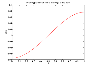
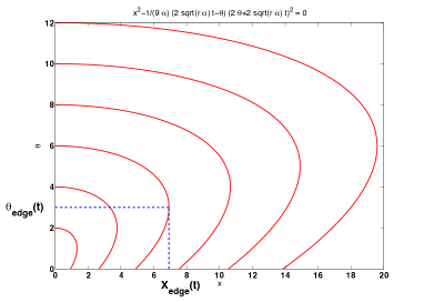
(a) (b)

Figure 1: (a) Phenotype selection. At the edge of the front the phenotypic distribution is not uniform: more motile individuals are selected. We solved numerically the relation dispersion for $(r,\alpha,\Theta)=(1,1,1)$. (b) Front acceleration. The set $\{u^{0}=0\}$ is plotted in the phase space $(x,\theta)$, for successive times. The far-right point $X_{\rm edge}(t)$ determines the location of the front.

3 Front acceleration

In the case where the set of dispersal rates is unbounded, say $\theta\in(0,+\infty)$, then we cannot solve the spectral problem (2). There is no intrinsic speed of propagation, and the front is accelerating as time goes on. Heuristically, we expect the averaged diffusion coefficient to grow linearly with time $\langle\theta\rangle\sim\left(\sqrt{\alpha r}\right)t$ (as for the Fisher-KPP equation set in the phenotype space). Hence the invasion front should scale as $\langle x\rangle\sim\left(\alpha^{1/4}r^{3/4}\right)t^{3/2}$ since the speed is given by $c\sim\sqrt{\langle\theta\rangle r}$. Therefore we perform the asymptotic scaling $(t,x,\theta)\to\left(t/\varepsilon,x/\varepsilon^{3/2},\theta/\varepsilon\right)$, in order to catch the motion of the front asymptotically. The equation writes after rescaling

$$\varepsilon\partial_{t}n^{\varepsilon}=\varepsilon^{2}\theta\partial^{2}_{xx}n^{\varepsilon}+rn^{\varepsilon}\left(1-\rho^{\varepsilon}(t,x)\right)+\varepsilon^{2}\alpha\partial^{2}_{\theta\theta}n^{\varepsilon}\,.$$ (6)

We perform the WKB ansatz in both variables $(x,\theta)$: $n^{\varepsilon}(t,x,\theta)=\exp\left(u^{\varepsilon}(t,x,\theta)/\varepsilon\right)$. We derive formally the Hamilton-Jacobi equation for $u^{0}$ in the limit $\varepsilon\to 0$:

$$\partial_{t}u^{0}-\theta|\partial_{x}u^{0}|^{2}-\alpha|\partial_{\theta}u^{0}|^{2}=r\left(1-\rho^{0}(t,x)\right)\,,$$ (7)

where $\rho^{0}(t,x)$ is the Lagrange multiplier associated with the constraint $\max_{\theta}u^{0}(t,x,\theta)\leq 0$. In particular, when the constraint is inactive, i.e. $\max_{\theta}u^{0}(t,x,\theta)<0$, we have $\rho^{0}(t,x)=0$. The behavior of the phase function $u^{0}(t,x,\theta)$ is as follows: the nullset $\{u^{0}(t,x,\theta)=0\}$ propagates in space and phenotype under the action of space mobility, and mutations, combined with growth of individuals. We are able to compute explicitely the evolution of this set for a particular initial data, using Lagrangian Calculus.

Proposition 2 (Front acceleration)

For the particular initial data, $u^{0}(0,x,\theta)=\begin{cases}0&\text{if $(x,\theta)=(0,0)$}\\ -\infty&\text{if $(x,\theta)\neq(0,0)$}\end{cases}$ the location of the nullset $\{u^{0}(t,x,\theta)=0\}$ is given by the following implicit formula (see Fig. 1)

$$x^{2}=\frac{1}{9\alpha}\left(\left(2\sqrt{r\alpha}\right)t-\theta\right)\left(2\theta+\left(2\sqrt{r\alpha}\right)t\right)^{2}\,.$$

Sketch of proof. The Hamiltonian is given by $H((x,\theta),(p_{x},p_{\theta}))=\theta|p_{x}|^{2}+\alpha|p_{\theta}|^{2}+r$, and the corresponding Lagrangian writes $L((x,\theta),(v_{x},v_{\theta}))=v_{x}^{2}/(4\theta)+v_{\theta}^{2}/(4\alpha)-r$. The system of characteristics is given by $\dot{X}(t)=(2\theta(t)p_{x}(t),2\alpha p_{\theta}(t))$, and $\dot{P}(t)=-(0,|p_{x}(t)|^{2})$. Using Lagrangian formulation, we deduce after some calculation that, with $Z$ the solution to equation $Z^{3}+(12\theta/\alpha)Z+24x/\alpha=0$, $u^{0}(t,x,\theta)$ is given by

$$u^{0}(t,x,\theta)=-\frac{1}{4\alpha t}\left(\theta+\frac{\alpha}{4}Z^{2}\right)^{2}\,.$$

This enables to compute the nullset $\{u^{0}(t,x,\theta)=0\}$. ∎

The far-right point of the curve is attained for $\theta_{\rm edge}=\left(\sqrt{r\alpha}\right)t$. This determines the location of the front. Hence the position of the front in space is exactly,

$$X_{\rm edge}(t)=\dfrac{4}{3}\left(\alpha^{1/4}r^{3/4}\right)t^{3/2}\,.$$

4 Adaptive dynamics at the edge of the front

Interestingly enough, the same equation (7) can be derived in the context of adaptive dynamics, a theory which studies mutation-selection processes. It is generally assumed that the mutation process is so slow that mutants can replace the resident species before new mutants arise, if they are better adapted to their environment. This yields a canonical equation which gives the dynamical evolution of the selected trait in the population [13, 14]. Recently, PDE-based methods have been successfully used to derive such a canonical equation for continuous mutation-selection processes [15, 16, 17]. Here we extend this theory to the case of front invasion coupled with a basic mutation process.

The only difference with (1) is that mutations are assumed to be rare ($\alpha\to\varepsilon^{2}\alpha$):

$$\partial_{t}n(t,x,\theta)=\theta\partial^{2}_{xx}n(t,x,\theta)+rn(t,x,\theta)\left(1-\rho(t,x)\right)+\varepsilon^{2}\alpha\partial^{2}_{\theta\theta}n(t,x,\theta)\,.$$

It is natural to perform a long time rescaling $t\to t/\varepsilon$ at the scale of evolutionary changes. Then it is useful to rescale space accordingly $x\to x/\varepsilon$ in order to catch the motion of the front (otherwise it would travel at order $O(1/\varepsilon)$). With these changes of scales, we end up again with equation (6), resp. (7) in the WKB limit. We restrict to the edge of the front, namely $\sup_{\theta}u^{0}(t,x,\theta)<0$, $\rho^{0}(t,x)=0$. We seek a canonical equation for the locally selected trait $\overline{\theta}(t,x)$ such that $u^{0}(t,x,\overline{\theta}(t,x))=\sup_{\theta}u^{0}(t,x,\theta)$.

Proposition 3 (Formal derivation of the canonical equation)

The locally selected trait $\overline{\theta}(t,x)$ formally satisfies a Burgers type equation with a source term,

$$\partial_{t}\overline{\theta}(t,x)-2\left(\overline{\theta}(t,x)\partial_{x}u^{0}\right)\partial_{x}\overline{\theta}(t,x)=\dfrac{|\partial_{x}u^{0}|^{2}}{-\partial^{2}_{\theta\theta}u^{0}}\,.$$ (8)

The speed of the transport equation is $-2\overline{\theta}(t,x)\partial_{x}u^{0}$. It coincides with the local minimal speed of the traveling front, see e.g. (5). The positive source term accounts for the evolutionary drift which pushes the population towards higher motility (numerical simulations not shown). This equation may yield shock wave singularities, as for the classical Burgers equation, because more motile populations, when located behind less motile populations, will invade them.

Proof. We start from the first order condition $\partial_{\theta}u^{0}(t,x,\overline{\theta}(t,x))=0$. We differentiate this relation with respect to $t$ and $x$, respectively,

$$\partial^{2}_{t\theta}u^{0}(t,x,\overline{\theta}(t,x))+\left(\partial^{2}_{\theta\theta}u^{0}\right)\partial_{t}\overline{\theta}(t,x)=0\,,\qquad\partial^{2}_{x\theta}u^{0}(t,x,\overline{\theta}(t,x))+\left(\partial^{2}_{\theta\theta}u^{0}\right)\partial_{x}\overline{\theta}(t,x)=0\,.$$

On the other hand, we differentiate equation (7) with respect to $\theta$,

$$\partial^{2}_{\theta t}u^{0}-|\partial_{x}u^{0}|^{2}-2\theta\partial_{x}u^{0}\partial^{2}_{\theta x}u^{0}-2\alpha\partial_{\theta}u^{0}\partial^{2}_{\theta\theta}u^{0}=0\,.$$

Evaluating the latter at $\theta=\overline{\theta}(t,x)$ yields

$$\partial^{2}_{\theta t}u^{0}-2\overline{\theta}(t,x)\partial_{x}u^{0}\partial^{2}_{\theta x}u^{0}=|\partial_{x}u^{0}|^{2}\,.$$

Combining these calculations, we conclude that $\overline{\theta}$ satisfies equation (8). ∎

Acknowledgements. S. M. benefits from a 2 year ”Fondation Mathématique Jacques Hadamard” (FMJH) postdoc scholarship. She would like to thank Ecole Polytechnique for its hospitality.

References

• [1] O. Bénichou, V. Calvez, N. Meunier, R. Voituriez, Front acceleration by dynamic selection in Fisher population waves, preprint.
• [2] J. Dockery, V. Hutson, K. Mischaikow, M. Pernarowski, The evolution of slow dispersal rates: a reaction diffusion model, J. Math. Biol. 37 (1) (1998) 61–83.
• [3] N. Champagnat, S. Méléard, Invasion and adaptive evolution for individual-based spatially structured populations, J. Math. Biol. 55 (2) (2007) 147–188.
• [4] A. Arnold, L. Desvillettes, C. Prévost, Existence of nontrivial steady states for populations structured with respect to space and a continuous trait, Commun. Pure Appl. Anal. 11 (1) (2012) 83–96.
• [5] A. D. Simmons, C. D. Thomas, Changes in dispersal during species’ range expansions, Amer. Nat. 164 (2004) 378–395.
• [6] H. Kokko, A. López-Sepulcre, From individual dispersal to species ranges: perspectives for a changing world, Science 313 (5788) (2006) 789–91.
• [7] O. Ronce, How does it feel to be like a rolling stone? Ten questions about dispersal evolution, Annu. Rev. Ecol. Syst. 38 (2007) 231–253.
• [8] R. Shine, G. P. Brown, B. L. Phillips, An evolutionary process that assembles phenotypes through space rather than through time, Proc Natl Acad Sci U S A 108 (14) (2011) 5708–11.
• [9] B. L. Phillips, G. P. Brown, J. K. Webb, R. Shine, Invasion and the evolution of speed in toads, Nature 439 (7078) (2006) 803.
• [10] E. Bouin, V. Calvez, A kinetic eikonal equation, Comptes Rendus Mathematique 350 (5–6) (2012) 243 – 248.
• [11] M. I. Freidlin, Geometric optics approach to reaction-diffusion equations, SIAM J. Appl. Math. 46 (2) (1986) 222–232.
• [12] L. C. Evans, P. E. Souganidis, A PDE approach to geometric optics for certain semilinear parabolic equations, Indiana Univ. Math. J. 38 (1) (1989) 141–172.
• [13] U. Dieckmann, R. Law, The dynamical theory of coevolution: a derivation from stochastic ecological processes, J Math Biol 34 (5-6) (1996) 579–612.
• [14] N. Champagnat, R. Ferrière, S. Méléard, From individual stochastic processes to macroscopic models in adaptive evolution, Stoch. Models 24 (suppl. 1) (2008) 2–44.
• [15] O. Diekmann, P.-E. Jabin, S. Mischler, B. Perthame, The dynamics of adaptation: an illuminating example and a hamilton-jacobi approach, Theor Popul Biol 67 (4) (2005) 257–71.
• [16] G. Barles, B. Perthame, Concentrations and constrained Hamilton-Jacobi equations arising in adaptive dynamics, in: Recent developments in nonlinear partial differential equations, Vol. 439 of Contemp. Math., Amer. Math. Soc., Providence, RI, 2007, pp. 57–68.
• [17] A. Lorz, S. Mirrahimi, B. Perthame, Dirac mass dynamics in multidimensional nonlocal parabolic equations, Comm. Partial Differential Equations 36 (6) (2011) 1071–1098.