Dichotomy for Holant* Problems with a Function on Domain Size 3

Abstract

Holant problems are a general framework to study the algorithmic complexity of counting problems. Both counting constraint satisfaction problems and graph homomorphisms are special cases. All previous results of Holant problems are over the Boolean domain. In this paper, we give the first dichotomy theorem for Holant problems for domain size $>2$. We discover unexpected tractable families of counting problems, by giving new polynomial time algorithms. This paper also initiates holographic reductions in domains of size $>2$. This is our main algorithmic technique, and is used for both tractable families and hardness reductions. The dichotomy theorem is the following: For any complex-valued symmetric function ${\bf F}$ with arity 3 on domain size 3, we give an explicit criterion on ${\bf F}$, such that if ${\bf F}$ satisfies the criterion then the problem ${\rm Holant}^{*}({\bf F})$ is computable in polynomial time, otherwise ${\rm Holant}^{*}({\bf F})$ is #P-hard.

1 Introduction

The study of computational complexity of counting problems has been a very active research area recently. Three related frameworks in which counting problems can be expressed as partition functions have received the most attention: Graph Homomorphisms (GH), Constraint Satisfaction Problems (CSP) and Holant Problems.

Graph Homomorphism was first defined by Lovász [37]. It captures a wide variety of graph properties. Given any fixed $k\times k$ symmetric matrix ${\bf A}$ over $\mathbb{C}$, the partition function $Z_{\bf A}$ maps any input graph $G=(V,E)$ to $Z_{\bf A}(G)=\sum_{\xi:V\rightarrow[k]}\hskip 1.9919pt\prod_{(u,v)\in E}{\bf A}_{\xi(u),\xi(v)}$. When ${\bf A}$ is a 0-1 matrix, then the product $\prod_{(u,v)\in E}$ is essentially a Boolean And function. The product value $\prod_{(u,v)\in E}{\bf A}_{\xi(u),\xi(v)}=0$ or 1, and it is 1 iff every edge $(u,v)\in E$ is mapped to an edge in the graph $H$ whose adjacency matrix is ${\bf A}$. Hence for a 0-1 matrix ${\bf A}$, $Z_{\bf A}(G)$ counts the number of “homomorphisms” from $G$ to $H$. For example, if ${\bf A}={\scriptsize\begin{bmatrix}1&1\\ 1&0\end{bmatrix}}$ then $Z_{\bf A}(G)$ counts the number of Independent Sets in $G$. If ${\bf A}={\tiny\begin{bmatrix}0&1&1\\ 1&0&1\\ 1&1&0\end{bmatrix}}$ then $Z_{\bf A}(G)$ is the number of valid 3-colorings. When ${\bf A}$ is not 0-1, $Z_{\bf A}(G)$ is a weighted sum of homomorphisms. Each ${\bf A}$ defines a graph property on graphs $G$. Clearly if $G$ and $G^{\prime}$ are isomorphic then $Z_{\bf A}(G)=Z_{\bf A}(G^{\prime})$. While individual graph properties are fascinating to study, Lovász’s intent is to study a wide class of graph properties representable as graph homomorphisms. The use of more general matrices ${\bf A}$ brings us into contact with another tradition, called partition functions of spin systems from statistical physics [3, 38]. The case of a $2\times 2$ matrix ${\bf A}={\scriptsize\begin{bmatrix}\beta&1\\ 1&\gamma\end{bmatrix}}$ is called a 2-spin system, and the special case $\beta=\gamma$ is the Ising model [31, 32, 28]. The Potts model with interaction strength $\gamma$ is defined by a $k\times k$ matrix ${\bf A}$ where all off-diagonal entries equal to 1 and all diagonal entries equal to $1+\gamma$ [27]. In classical physics, the matrix ${\bf A}$ is always real-valued. However, in a generic quantum system for which complex numbers are the right language, the partition function is in general complex-valued [24]. In particular, if the physics model is over a discrete graph and is non-orientable, then the edge weights are given by a symmetric complex matrix. We will see that the use of complex numbers is not just a modeling issue, it provides an inner unity in the algorithmic theory of partition functions.

A more general framework than GH is called counting CSP. Let ${\cal F}$ be any finite set of (complex-valued) constraint functions defined on some domain set $D$. It defines a counting CSP problem ${\rm\#CSP}({\cal F})$: An input consists of a bipartite graph $G=(X,Y,E)$, each $x\in X$ is a variable on $D$, each $y\in Y$ is labeled by a constraint function $f\in{\cal F}$, and the edges in $E$ indicate how each constraint function is applied. The output is the sum of product of evaluations of the constraint functions over all assignments for the variables [17, 7, 19, 6, 14, 21, 11]. Again if all constraint functions in ${\cal F}$ are 0-1 valued then it counts the number of solutions. In general, this sum of product a.k.a. partition function is a weighted sum of solutions, and has occupied a central position. It reaches many areas ranging from AI, machine learning, tensor networks, statistical physics and coding theory. Note that GH is the special case where ${\cal F}$ consists of a single binary symmetric function.

The strength of these frameworks derives from the fact that they can express many problems of interest and simultaneously it is possible to achieve a complete classification of its worst case complexity.

While GH (or spin systems) can express a great variety of natural counting problems, Freedman, Lovász and Schrijver [25] showed that GH cannot express the problem of counting Perfect Matchings. It is well known that the FKT algorithm [35, 41] can count the number of perfect matchings in a planar graph in polynomial time. This is one basic component of holographic algorithms recently introduced by Valiant [43, 42]. (The second basic component is holographic reduction.) To capture this extended class of problems typified by Perfect Matchings, the framework of Holant problems was introduced [13, 14, 15]. Briefly, an input instance of a Holant problem is a graph $G=(V,E)$ where each edge represents a variable and each vertex is labeled by a constraint function. The partition function is again the sum of product of the constraint function evaluations, over all edge assignments. E.g., if edges are Boolean variables (i.e., domain size 2), and the constraint function at every vertex is the Exact-One function which is 1 if exactly one incident edge is assigned true and 0 otherwise, then the partition function counts the number of perfect matchings. If each vertex has the At-Most-One function then it counts all (not necessarily perfect) matchings. It can be shown easily that the Holant framework can simulate spin systems but, as shown by [25], the converse is not true. The Holant framework turns out to be a very natural setting and captures many interesting problems. E.g., it was independently discovered in coding theory, where it is called Normal Factor Graphs or Forney Graphs [33, 34, 2, 1].

A complexity dichotomy theorem for counting problems classifies every problem within a class to be either in P or #P-hard. For GH, this is proved for $Z_{\bf A}$ for all symmetric complex matrices ${\bf A}$ [10]. This is a culmination of a long series of results [20, 8, 26]. The proof of [10] is difficult, but the tractability criterion is very explicit: $Z_{\bf A}$ is in polynomial time if ${\bf A}$ is a suitable rank-one modification of a tensor product of Fourier matrices, and is #P-hard otherwise. Explicit dichotomy theorems were also proved for counting CSP on the Boolean domain (i.e., $|D|=2$): unweighted [17], non-negative weighted [19], real weighted [4], and finally complex weighted [14], where holographic reductions played an important role in the final result. Complex numbers make their appearance naturally as eigenvalues, and provide an internal logic to the theory, even if one is only interested in 0-1 valued constraint functions.

When we go from the Boolean domain to domain size $>2$, there is a huge increase in difficulty to prove dichotomy theorems. This is already seen in decision CSP, where the dichotomy (i.e., any decision CSP is either in P or NP-complete) for the Boolean domain is Schaefer’s theorem [39], but the dichotomy for domain size 3 is a major achievement by Bulatov [5]. A long standing conjecture by Feder and Vardi [23] states that a dichotomy for decision CSP holds for all domain size, but this is open for domain size $>3$. The assertion that every decision CSP is either solvable in polynomial time or NP-complete is by no means obvious, since assuming P $\not=$ NP, Ladner showed that NP contains problems that are neither in P nor NP-complete [36]. This is also valid for P versus #P.

With respect to counting problems, for any finite set of 0-1 valued functions $\cal F$ over a general domain, Bulatov [6] proved a dichotomy theorem for ${\rm\#CSP}({\cal F})$, which uses deep results from Universal Algebra. Dyer and Richarby [21, 22] gave a more direct proof which has the advantage that their tractability criterion is decidable. Decidable dichotomy theorems are more desirable since they tell us not only every ${\cal F}$ belongs to either one or the other class, but also how to decide for a given ${\cal F}$ which class it belongs to. A decidable dichotomy theorem for ${\rm\#CSP}({\cal F})$, where all functions in $\cal F$ take non-negative values, is given in [11]. Finally a dichotomy theorem for all complex-valued ${\rm\#CSP}({\cal F})$ is proved in [9]. This last dichotomy is not known to be decidable.

More than giving a formal classification, the deeper meaning of a dichotomy theorem is to provide a comprehensive structural understanding as to what makes a problem easy and what makes it hard. This deeper understanding goes beyond the validity of a dichotomy, and even more than decidability, which is: Given $\cal F$, decide whether it satisfies the tractability criterion so that ${\rm\#CSP}({\cal F})$ is in P. Ideally we hope for dichotomy theorems that are explicit in the sense that the tractability criteria provide a mathematical characterization that can be applied symbolically to an arbitrary $\cal F$. An explicit dichotomy can also be readily used to prove broader dichotomy theorems, as we will see in this paper. The known dichotomy theorems for GH [10] and for CSP on general domains have very different flavors. Dichotomy theorems for ${\rm\#CSP}({\cal F})$ for all domain size $>2$ are not explicit. The tractability criterion is infinitary. This is in marked contrast with the dichotomy theorems for GH. For Holant problems all previous results are over the Boolean domain and are mostly explicit. In this paper, we give the first dichotomy theorem for Holant problems for domain size $>2$, and it is explicit.

Our main theorem can be stated as follows: For any complex-valued symmetric function ${\bf F}$ with arity 3 on domain size 3, we give an explicit criterion on ${\bf F}$, such that if ${\bf F}$ satisfies the criterion then the problem ${\rm Holant}^{*}({\bf F})$ is computable in polynomial time, otherwise ${\rm Holant}^{*}({\bf F})$ is #P-hard. (Formal definitions will be given in Section 2.) It is known that in the Holant framework any set of binary functions is tractable. A ternary function is the basic setting in the Holant framework where both tractable and intractable cases occur. A single ternary function in the Holant framework is the analog of GH as the basic setting in the CSP framework with a single binary function. Therefore this case is interesting in its own right. Furthermore, as demonstrated many times in the Boolean domain [14, 15, 12, 29, 30], a dichotomy for a single ternary function serves as the starting point for more general dichotomies in the Holant framework.

In order to prove this dichotomy theorem, we have to discover new tractable classes of Holant problems, and design new polynomial time algorithms. Many intricacies of the interplay between tractability and intractability do not occur in the Boolean domain. However these new algorithms actually provide fresh insight to our previous dichotomy theorems for the Boolean domain. They offer a deeper and more complete understanding of what makes a problem easy and what makes it hard.

Our main algorithmic innovation is to initiate the theory of holographic reductions in domains of size $>2$. It is a recurring theme in our proof techniques here. This is a new development; all previous work on holographic algorithms and reductions have been on the Boolean domain. Holographic transformation offers a perspective on internal connections and equivalences between different looking problems, that is unavailable by any other means. In particular since it naturally uses eigenvalues and eigenvectors, the field of complex numbers $\mathbb{C}$ is the natural setting to formulate the class of problems, even if one is only interested in 0-1 valued or non-negative valued constraint functions. Using complex-valued constraints in defining Holant problems we can see the internal logical connections between various problems. Completely different looking problems can be seen as one and the same problem under holographic transformations. The proof of our dichotomy theorem would be impossible without working over $\mathbb{C}$. Even the dichotomy criterion would be impossible to state without it. To quote Jacques Hadamard: “The shortest path between two truths on the real line passes through the complex plane.”

Suppose our domain set is $\{B,G,R\}$, named for the three colors Blue, Green and Red. We isolate several classes of tractable cases of ${\bf F}$. One of them is a generalization of Fibonacci signatures from the Boolean domain, under an orthogonal transformation. Another involves a concept called isotropic vectors, which self-annihilates under dot product. The third type involves a more intricate interplay between an isotropic vector in some dimension and another function primarily “living” in the other dimensions. This last type was only discovered after we failed to push through certain hardness proofs.

For hardness proofs, the first main idea is to construct a binary function which acts as an Equality function when restricted to $\{G,R\}$, and is zero elsewhere. This construction allows us to restrict a function on $\{B,G,R\}$ to a domain of size 2, and employ the known (and explicit) dichotomy theorems for the Boolean domain. The plan is to use it to restrict ${\bf F}$ to $\{G,R\}$ and, assuming it is non-degenerate, to anchor the entire hardness proof on that. Here it is crucial that the known Boolean domain dichotomy is explicit. This part of the proof is quite demanding and heavily depends on holographic reductions. A central motif is to show that after a holographic reduction, ${\bf F}$ must possess fantastic regularity to escape #P-hardness.

What perhaps took us by surprise is that when ${\bf F}$ restricted to $\{G,R\}$ is degenerate, there is still considerable technical difficulty remaining. These are eventually overcome by using unsymmetric functions.

This work has been a marathon for us. During the process, repeatedly, we failed to clinch the hardness proof for some subclasses of functions and then new tractable cases were found. So we had to reformulate the final dichotomy several times. The discovery process is mutually reinforcing between new algorithms and hardness proofs. On many occasions we believed that we had overcome one last hurdle, only to be stymied by yet another. However the struggle has also paid handsome dividends. For example, our SODA paper two years ago [16] was obtained as part of the program to achieve this dichotomy. We realized we needed a dichotomy for unsymmetric functions over the Boolean domain, and indeed that is used to overcome a major difficulty in the proof here.

2 Preliminary

2.1 Definitions

Definitions of Holant problem and gadget are introduced in this subsection. The readers who are familiar with the definitions in [15, 16] may skip.

Let $D$ be a finite domain set, and $\cal F$ be a finite set of constraint functions called signatures. Each $\mathbf{F}\in{\cal F}$ is a mapping from $D^{k}\to\mathbb{C}$ for some arity $k$. We assume signatures take complex algebraic numbers.

A signature grid $\Omega=(G,{\cal F},\pi)$ consists of a graph $G=(V,E)$ where each vertex $v\in V$ is labeled by a function $\mathbf{F}_{v}\in\mathbb{C}$, and $\pi$ is the labeling. The Holant problem on instance $\Omega$ is to evaluate

$${\rm Holant}_{\Omega}=\sum_{\sigma}\prod_{v\in V}\mathbf{F}_{v}(\sigma\mid_{E(v)}),$$ (1)

a sum over all edge assignments $\sigma:E\rightarrow D$, where $E(v)$ denotes the incident edges at $v$.

A function $\mathbf{F}_{v}$ is listed by its values lexicographically as a truth table, or as a tensor in $(\mathbb{C}^{|D|})^{\otimes\deg(v)}$. We can identify a unary function $\mathbf{F}(x):D\rightarrow\mathbb{C}$ with a vector ${\bf u}\in\mathbb{C}^{|D|}$. Given two vectors ${\bf u}$ and ${\bf v}$ of dimension $|D|$, the tensor product ${\bf u}\otimes{\bf v}$ is a vector in $\mathbb{C}^{|D|^{2}}$, with entries $u_{i}v_{j}$ ($1\leq i,j\leq|D|$). For matrices $A=(a_{i,j})$ and $B=(b_{k,l})$, the tensor product (or Kronecker product) $A\otimes B$ is defined similarly; it has entries $a_{i,j}b_{k,l}$ indexed by $((i,k),(j,l))$ lexicographically. We write ${\bf u}^{\otimes k}$ for ${\bf u}\otimes\ldots\otimes{\bf u}$ with $k$ copies of ${\bf u}$. $A^{\otimes k}$ is similarly defined. We have $(A\otimes B)(A^{\prime}\otimes B^{\prime})=(AA^{\prime}\otimes BB^{\prime})$ whenever the matrix products are defined. In particular, $A^{\otimes k}({\bf u}_{1}\otimes\ldots\otimes{\bf u}_{k})=A{\bf u}_{1}\otimes\ldots\otimes A{\bf u}_{k}$ when the matrix-vector products $A{\bf u}_{i}$ are defined.

A signature $\mathbf{F}$ of arity $k$ is degenerate if $\mathbf{F}={\bf u}_{1}\otimes{\bf u}_{2}\otimes\ldots\otimes{\bf u}_{k}$ for some vectors ${\bf u}_{i}$. Equivalently there are unary functions $\mathbf{F}_{i}$ such that $\mathbf{F}(x_{1},\ldots,x_{k})=\mathbf{F}_{1}(x_{1})\cdots\mathbf{F}_{k}(x_{k})$. Such a signature is very weak; there is no interaction between the variables. If every function in ${\cal F}$ is degenerate, then ${\rm Holant}_{\Omega}$ for any $\Omega=(G,{\cal F},\pi)$ is computable in polynomial time in a trivial way: Simply split every vertex $v$ into $\deg(v)$ many vertices each assigned a unary $\mathbf{F}_{i}$ and connected to the incident edge. Then ${\rm Holant}_{\Omega}$ becomes a product over each component of a single edge. Thus degenerate signatures are weak and should be properly understood as made up by unary signatures. To concentrate on the essential features that differentiate tractability from intractability, we introduced Holant^∗ problems [14, 15]. These are Holant problems where unary signatures are assumed to be present.

We consider a type of graphs $G=(V,I,E)$ with two kinds of edges. Edges in $I$ are ordinary internal edges with two endpoints. Edges in $E$ are external edges (also called dangling edges) which have only one endpoint in $V$. Such a graph can be made into a part of a larger graph as follows. Given a graph $G^{\prime}$, we can replace a vertex $v$ of $G^{\prime}$ by a graph $G$ with external edges, merging the external edges with the incident edges of $v$. Reversely, when some edges are cut from a graph, the cut edges become external edges on both sides. When two external edges are connected, they merge to become one edge.

A gadget consists of a graph $G=(V,I,E)$ and a labeling $\pi$, where each vertex $v\in V$ is labeled by a function $\mathbf{F}_{v}\in\mathbb{C}$. A gadget can be a part of a signature grid. For example, in a signature grid, a single vertex of degree $d$ constitutes a gadget. It has the single vertex, together with its function, an empty $I$ set, and its $d$ incident edges as external edges. It can be replaced by a gadget $G$ with $|E|=d$ and vice versa. In a signature grid, when we want to replace a gadget $G$ with $|E|=d$ by a vertex $v$ of degree $d$, what is the right function $\mathbf{F}_{v}$ that keeps the value of the signature grid unchanged? The function of a gadget is defined to have this property, and it is also a natural generalization of Holant.

On an assignment $\tau:E\rightarrow D$, the function $\mathbf{F}_{G}$ of a gadget $G$ has value

$$\mathbf{F}_{G}(\tau)=\sum_{\sigma}\prod_{v\in V}\mathbf{F}_{v}(\tau\sigma\mid_{E(v)}),$$

a sum over all edge assignments $\sigma:I\rightarrow D$, and $\tau\sigma$ is the combined assignment on $E\cup I$.

Suppose one gadget is the disjoint union of two parts, each has two external edges. Suppose the binary functions (on $x_{1},x_{2}$ and $x_{3},x_{4}$ respectively) in matrix form are $\mathbf{A}$ and $\mathbf{B}$. Then the function of this gadget is $\mathbf{F}_{x_{1}x_{3},x_{2}x_{4}}=\mathbf{A}_{x_{1},x_{2}}\otimes\mathbf{B}_{x_{3},x_{4}}$, where $\mathbf{F}_{x_{1}x_{3},x_{2}x_{4}}$ denotes the matrix with two indices $x_{1}x_{3}$ and $x_{2}x_{4}$, and the value of this entry is just $\mathbf{F}(x_{1},x_{2},x_{3},x_{4})$.

Another example is the following. There are two binary functions $\mathbf{A}$ and $\mathbf{B}$. They share an internal edge $x_{2}$. Other two edges $x_{1},x_{3}$ are external. The function of this gadget is $\mathbf{F}(x_{1},x_{3})=\sum_{x_{2}}\mathbf{A}(x_{1},x_{2})\mathbf{A}(x_{2},x_{3})$, that is, $\mathbf{F}_{x_{1},x_{3}}=\mathbf{A}_{x_{1},x_{2}}\mathbf{A}_{x_{2},x_{3}}$, the matrix product.

2.2 Holographic Reduction

To introduce the idea of holographic reductions, it is convenient to consider bipartite graphs. For a general graph, we can always transform it into a bipartite graph preserving the Holant value, as follows: For each edge in the graph, we replace it by a path of length $2$, and assign to the new vertex the binary Equality function $(=_{2})$.

We use ${\rm Holant}(\mathcal{R}\mid\mathcal{G})$ to denote the Holant problem on bipartite graphs $H=(U,V,E)$, where each signature for a vertex in $U$ or $V$ is from $\mathcal{R}$ or $\mathcal{G}$, respectively. An input instance for the bipartite Holant problem is a bipartite signature grid and is denoted as $\Omega=(H;\ \mathcal{R}\mid\mathcal{G};\ \pi)$. Signatures in $\mathcal{R}$ are considered as row vectors (or covariant tensors); signatures in $\mathcal{G}$ are considered as column vectors (or contravariant tensors) [18].

For a $|D|\times|D|$ matrix $T$ and a signature set $\mathcal{F}$, define $T\mathcal{F}=\{\mathbf{G}\mid\exists\mathbf{F}\in\mathcal{F}$ of arity $n,~{}\mathbf{G}=T^{\otimes n}\mathbf{F}\}$, similarly for $\mathcal{F}T$. Whenever we write $T^{\otimes n}\mathbf{F}$ or $T\mathcal{F}$, we view the signatures as column vectors; similarly for $\mathbf{F}T^{\otimes n}$ or $\mathcal{F}T$ as row vectors. A holographic transformation by $T$ is the following operation: given a signature grid $\Omega=(H;\ \mathcal{R}\mid\mathcal{G};\ \pi)$, for the same graph $H$, we get a new grid $\Omega^{\prime}=(H;\ \mathcal{R}T\mid T^{-1}\mathcal{G};\ \pi)$ by replacing each signature in $\mathcal{R}$ or $\mathcal{G}$ with the corresponding signature in $\mathcal{R}T$ or $T^{-1}\mathcal{G}$.

Theorem 2.1 (Valiant’s Holant Theorem [43]).

If there is a holographic transformation mapping signature grid $\Omega$ to $\Omega^{\prime}$, then ${\rm Holant}_{\Omega}={\rm Holant}_{\Omega^{\prime}}$.

Therefore, an invertible holographic transformation does not change the complexity of the Holant problem in the bipartite setting. We illustrate the power of holographic transformation by an example. Let $\mathbf{F}=[\frac{3}{2},0,\frac{1}{2},0,\frac{3}{2}]$. Consider ${\rm Holant}(\mathbf{F})$ on the Boolean domain. For a 4-regular graph $G$, ${\rm Holant}(\mathbf{F})$ is a sum over all 0-1 edge assignments of products of local evaluations. Each vertex contributes a factor $\frac{3}{2}$ if all incident edges are assigned the same truth value, a factor $\frac{1}{2}$ if exactly half are assigned 1 and the other half 0. Before anyone consigns this problem to be artificial and unnatural, consider a holographic transformation by $Z=\frac{1}{\sqrt{2}}{\scriptsize\begin{bmatrix}1&1\\ i&-i\end{bmatrix}}$. Then ${\rm Holant}(\mathbf{F})={\rm Holant}(=_{2}\mid\mathbf{F})={\rm Holant}((=_{2})Z^{\otimes 2}\mid(Z^{-1})^{\otimes 4}\mathbf{F})$. Let $\hat{\mathbf{F}}=[0,0,1,0,0]$, and writing it as a symmetrized sum of tensor products, then

$$Z^{\otimes 4}\hat{\mathbf{F}} =Z^{\otimes 4}{\scriptsize\left\{\begin{bmatrix}1\\ 0\end{bmatrix}\otimes\begin{bmatrix}1\\ 0\end{bmatrix}\otimes\begin{bmatrix}0\\ 1\end{bmatrix}\otimes\begin{bmatrix}0\\ 1\end{bmatrix}+\begin{bmatrix}1\\ 0\end{bmatrix}\otimes\begin{bmatrix}0\\ 1\end{bmatrix}\otimes\begin{bmatrix}1\\ 0\end{bmatrix}\otimes\begin{bmatrix}0\\ 1\end{bmatrix}+\dotsb+\begin{bmatrix}0\\ 1\end{bmatrix}\otimes\begin{bmatrix}0\\ 1\end{bmatrix}\otimes\begin{bmatrix}1\\ 0\end{bmatrix}\otimes\begin{bmatrix}1\\ 0\end{bmatrix}\right\}}$$

$$=\tfrac{1}{4}{\scriptsize\left\{\begin{bmatrix}1\\ i\end{bmatrix}\otimes\begin{bmatrix}1\\ i\end{bmatrix}\otimes\begin{bmatrix}1\\ -i\end{bmatrix}\otimes\begin{bmatrix}1\\ -i\end{bmatrix}+\begin{bmatrix}1\\ i\end{bmatrix}\otimes\begin{bmatrix}1\\ -i\end{bmatrix}\otimes\begin{bmatrix}1\\ i\end{bmatrix}\otimes\begin{bmatrix}1\\ -i\end{bmatrix}+\dotsb+\begin{bmatrix}1\\ -i\end{bmatrix}\otimes\begin{bmatrix}1\\ -i\end{bmatrix}\otimes\begin{bmatrix}1\\ i\end{bmatrix}\otimes\begin{bmatrix}1\\ i\end{bmatrix}\right\}}$$

$$=\tfrac{1}{2}[3,0,1,0,3]=\mathbf{F};$$

Hence the contravariant transformation $(Z^{-1})^{\otimes 4}\mathbf{F}=\hat{\mathbf{F}}$. Meanwhile, a covariant transformation by $Z$ transforms $(=_{2})$ to the binary Disequality function $(\neq_{2})$

$$(=_{2})Z^{\otimes 2}={\scriptsize\begin{pmatrix}1&0&0&1\end{pmatrix}}Z^{\otimes 2}={\scriptsize\left\{\begin{pmatrix}1&0\end{pmatrix}^{\otimes 2}+\begin{pmatrix}0&1\end{pmatrix}^{\otimes 2}\right\}}Z^{\otimes 2}=\tfrac{1}{2}{\scriptsize\left\{\begin{pmatrix}1&1\end{pmatrix}^{\otimes 2}+\begin{pmatrix}i&-i\end{pmatrix}^{\otimes 2}\right\}}=[0,1,0]=(\neq_{2}).$$

So ${\rm Holant}(\mathbf{F})={\rm Holant}((\neq_{2})\mid[0,0,1,0,0])$; they are really one and the same problem. A moment’s reflection shows that this latter formulation is counting the number of Eulerian orientations on 4-regular graphs, an eminently natural problem!

Furthermore, holographic transformation by an orthogonal matrix $T$ preserves the binary equality and thus can be used freely in the standard setting.

Theorem 2.2.

Suppose $T$ is an orthogonal matrix $(TT^{\tt T}=I)$ and let $\Omega=(G,\mathcal{F},\pi)$ be a signature grid. Under a holographic transformation by $T$, we get a new grid $\Omega^{\prime}=(G,T\mathcal{F},\pi)$ and ${\rm Holant}_{\Omega}={\rm Holant}_{\Omega^{\prime}}$.

When $T$ has a special $\{B\}$ and $\{G,R\}$ domain separated form, we observe that each $\{G,R\}$-line in the table for $T^{\otimes 3}\mathbf{F}$ and $\mathbf{F}$, which correspond to a fixed number of $B$ assigned, are closely related by the $\{G,R\}$-block of $T$, as stated in the following Fact. We call this a domain separated holographic reduction .

Fact 1.

Suppose $T$ is in the $\{B\}$ and $\{G,R\}$ domain separated form, $\left(\begin{matrix}e&0&0\\ 0&a&b\\ 0&c&d\end{matrix}\right)$. Let $M=\left(\begin{matrix}a&b\\ c&d\end{matrix}\right)$. We have,

$$(T^{\otimes 3}\mathbf{F})^{*\rightarrow\{G,R\}} = M^{\otimes 3}(\mathbf{F}^{*\rightarrow\{G,R\}}),$$

$$(T^{\otimes 3}\mathbf{F})^{1=B,2,3\rightarrow\{G,R\}} = eM^{\otimes 2}(\mathbf{F}^{1=B,2,3\rightarrow\{G,R\}}),$$

$$(T^{\otimes 3}\mathbf{F})^{1=B,2=B,3\rightarrow\{G,R\}} = e^{2}M(\mathbf{F}^{1=B,2=B,3\rightarrow\{G,R\}}).$$

Proof.

We prove the second formula as an example. Other formulae can be proved similarly.

$(T^{\otimes 3}\mathbf{F})^{1=B,2,3\rightarrow\{G,R\}}$ is the line $[(T^{\otimes 3}\mathbf{F})_{BGG},(T^{\otimes 3}\mathbf{F})_{BGR},(T^{\otimes 3}\mathbf{F})_{BRR}]$ in the triangular table form of $T^{\otimes 3}\mathbf{F}$, and $\mathbf{F}^{1=B,2,3\rightarrow\{G,R\}}$ is the corresponding line of $\mathbf{F}$.

Because one input of $T^{\otimes 3}\mathbf{F}$ is fixed to $B$, it is equivalent to connecting one unary function $(1,0,0)$ to $T^{\otimes 3}\mathbf{F}$. By associativity this unary can be combined with a copy of $T$ in the gadget $T^{\otimes 3}\mathbf{F}$. This combination results in a unary function $\langle(1,0,0),T\rangle=(T_{B,B},0,0)=(e,0,0)$, which is then connected to $\mathbf{F}$. This creates a binary function $e\mathbf{F}^{1=B}$. Now, we get $(T^{\otimes 2}(e\mathbf{F}^{1=B}))^{*\rightarrow\{G,R\}}$. The two external edges of the gadget $T^{\otimes 2}(e\mathbf{F}^{1=B})$ are restricted to $\{G,R\}$. Because the domain of $T$ is separated into $\{B\}$ and $\{G,R\}$, they force the two internal edges to take values in $\{G,R\}$. Since all 4 edges take values in $\{G,R\}$, this turns $T^{\otimes 2}(e\mathbf{F}^{1=B})$ into $eM^{\otimes 2}\mathbf{F}^{1=B,2,3\rightarrow\{G,R\}}$. ∎

2.3 Notations

A signature $\mathbf{F}$ on $r$ variables is symmetric if $\mathbf{F}(x_{1},\ldots,x_{r})=\mathbf{F}(x_{\sigma(1)},\ldots,x_{\sigma(r)})$ for all $\sigma\in\mathfrak{S}_{k}$, the symmetric group. It can be shown easily that a symmetric signature $\mathbf{F}$ is degenerate iff $\mathbf{F}={\bf u}^{\otimes r}$ for some unary ${\bf u}$.

We use $\rm{Sym}(\mathbf{F})$ to denote the symmetrization of $\mathbf{F}$ as follows: For $i_{1},i_{2},\ldots,i_{r}\in\{B,G,R\}$,

$${(\rm{Sym}(\mathbf{F}))}_{(i_{1}i_{2}\ldots i_{r})}=\sum_{\sigma\in\mathfrak{S}_{r}}F_{i_{\sigma 1}i_{\sigma 2}\cdots i_{\sigma r}},$$

where the summation is over the symmetric group $\mathfrak{S}_{r}$ on $r$ symbols.

If $\mathbf{F}$ is degenerate, given as a simple tensor product

$$\mathbf{F}=v_{1}\otimes v_{2}\otimes\cdots\otimes v_{r},$$

then the symmetrization of $\mathbf{F}$ is the symmetric product of the factors:

$${\rm{Sym}(\mathbf{F})}=\sum_{\sigma\in\mathfrak{S}_{r}}v_{{\sigma 1}}\otimes v_{{\sigma 2}}\otimes\cdots\otimes v_{{\sigma r}}.$$

We consider a function $\mathbf{F}$ and its nonzero multiple $c\mathbf{F}$ as the same function, as $c\mathbf{F}$ only introduces a easily computable global factor.

A symmetric signature $\mathbf{F}$ on $r$ Boolean variables can be expressed as $[f_{0},f_{1},\dotsc,f_{k}]$, where $f_{j}$ is the value of $\mathbf{F}$ on inputs of Hamming weight $j$. In the following, we focus on symmetric signatures over domain $[3]$. We use three symbols $\{B,G,R\}$ to denote the domain elements.

Let $\mathbf{F}$ be a symmetric signatures of arity $3$ over domain $\{B,G,R\}$. We use the following notation for $\mathbf{F}$.

$$\mathbf{F}=[F_{BBB};F_{BBG},F_{BBR};F_{BGG},F_{BGR},F_{BRR};F_{GGG},F_{GGR},F_{GRR},F_{RRR}].$$

Alternatively we also use the following notation:

$$F_{BBB}$$

(2)

This notation can be extended to other arities. For a signature with arity two, we also use a symmetric $q\times q$ matrix to represent it.

$$\mathbf{F} = [F_{BB};F_{BG},F_{BR};F_{GG},F_{GR},F_{RR}]$$

$$= \begin{bmatrix}F_{BB}&F_{BG}&F_{BR}\\ F_{BG}&F_{GG}&F_{GR}\\ F_{BR}&F_{GR}&F_{RR}\end{bmatrix}.$$

For a binary signature, the rank of the signature is the rank of its $q\times q$ matrix.

A unary function can be represented as $[F_{B};F_{G},F_{R}]$ in symmetric notation, or simply $(F_{B},F_{G},F_{R})$ in full version.

We use $\mathbf{F}^{i=A}$, where $i\in[r]$ and $A\in\{B,G,R\}$, to denote a signature of arity $r-1$ by fixing the $i$-th input of $\mathbf{F}$ to $A$. For example for the $\mathbf{F}$ in (2)

$$\mathbf{F}^{1=B}=\begin{bmatrix}F_{BBB}&F_{BBG}&F_{BBR}\\ F_{BBG}&F_{BGG}&F_{BGR}\\ F_{BBR}&F_{BGR}&F_{BRR}\end{bmatrix}.$$ (3)

Sometimes, we also restrict the $i$-th input of $\mathbf{F}$ to $S$, a subset of $\{B,G,R\}$, and we use $\mathbf{F}^{i\rightarrow S}$ (for example $\mathbf{F}^{2\rightarrow\{B,R\}}$) to denote it. We use $\mathbf{F}^{*\rightarrow{S}}$ to denote the case when we restrict all inputs of $\mathbf{F}$ to $S$. For example

$$\mathbf{F}^{*\rightarrow\{G,R\}}=[F_{GGG},F_{GGR},F_{GRR},F_{RRR}].$$

The above notation can be combined, for example

$$\mathbf{F}^{1=B;2,3\rightarrow\{G,R\}}=[F_{BGG},F_{BGR},F_{BRR}].$$

We also use $F_{a,b,c}$, ($a,b,c\in\mathbf{N},a+b+c=r$) to denote the value of $\mathbf{F}$ when the numbers of $B$’s, $G$’s and $R$’s among the inputs are respectively $a$, $b$ and $c$. For example, $F_{1,2,0}=F_{BGG}$.

Definition 2.3.

A symmetric function $F$ of arity $r\geq 2$, gives a $r$-uniform hyper graph $G$ whose vertex set is the domain of variables. We say two disjoint subsets of domain are separated, if they are contained in different connected components of $G$.

For example, if a ternary function has the form

			$F_{BBB}$
		$0$		$0$
	$0$		$0$		$0$
$F_{GGG}$		$F_{GGR}$		$F_{GRR}$		$F_{RRR}$

We say that $B$ is separated from $\{G,R\}$.

2.4 A Calculus with Symmetric Signatures

In order to follow the proofs in this paper, it would be helpful to familiarize oneself with a certain calculus that lets us reason about these symmetric signatures on domain size 3. We will mainly illustrate it with signatures of arity 2 or 3. It is easy to generalize it to any higher arities.

For any symmetric signature $\mathbf{F}$ of arity 2 on domain $\{B,G,R\}$, we make the following identification of the notation

		$F_{BB}$
	$F_{BG}$		$F_{BR}$
$F_{GG}$		$F_{GR}$		$F_{RR}$

with its matrix form

$$\begin{bmatrix}F_{BB}&F_{BG}&F_{BR}\\ F_{BG}&F_{GG}&F_{GR}\\ F_{BR}&F_{GR}&F_{RR}\end{bmatrix}.$$

We note that the three corners in counterclock-wise order $B,G,R$ are listed on the main diagonal in the matrix. Then the off-diagonal entries are filled by the corresponding color pairs, e.g., the entry $F_{BG}$ between $B$ and $G$ are filled at the $(B,G)$ and $(G,B)$ entry of the matrix.

Let $\mathbf{F}$ be a ternary symmetric signature, and let $\mathbf{u}=(\alpha,\beta,\gamma)$ be a unary signature, both on domain $\{B,G,R\}$, we can form a binary symmetric signature by connecting one input of $\mathbf{F}$ with $\mathbf{u}$. Since $\mathbf{F}$ is symmetric, connecting to any one of the input wires defines the same symmetric signature on the other input wires. We denote this signature by $\langle\mathbf{u},\mathbf{F}\rangle$. By symmetry, for $\mathbf{F}$ of arity at least 2, $\langle\mathbf{v},\langle\mathbf{u},\mathbf{F}\rangle\rangle=\langle\mathbf{u},\langle\mathbf{v},\mathbf{F}\rangle\rangle$.

Suppose $\mathbf{F}$ is given in (2). Then $\langle\mathbf{u},\mathbf{F}\rangle$ is the following

		$F^{\prime}_{BB}$
	$F^{\prime}_{BG}$		$F^{\prime}_{BR}$
$F^{\prime}_{GG}$		$F^{\prime}_{GR}$		$F^{\prime}_{RR}$

where each entry $F^{\prime}_{XY}$ is obtained by a linear combination $\alpha F_{XYB}+\beta F_{XYG}+\gamma F_{XYR}$; i.e., we start at any entry on the first three rows in the triangular table for $\mathbf{F}$, and then form a linear combination with coefficients $\alpha,\beta,\gamma$ in a counterclock-wise order involving the three entries forming a small triangle. E.g., start with entry $F_{BBG}$, we get $F^{\prime}_{BG}=\alpha F_{BBG}+\beta F_{BGG}+\gamma F_{BGR}$.

Suppose $\mathbf{F}$ is a symmetric ternary signature, and $\mathbf{u}=(1,i,0)$. Then we see immediately that $\langle\mathbf{u},\mathbf{F}\rangle=\mathbf{0}$ (the zero binary function) iff $\mathbf{F}$ has the following form

$$x$$

(4)

Fixing some variables to $R$ and restrict others to $\{B,G\}$, we get $\mathbf{F}^{1,2,3\rightarrow\{B,G\}}=[x,xi,-x,-xi]$, $\mathbf{F}^{1=R;2,3\rightarrow\{B,G\}}=[y,yi,-y]$ and $\mathbf{F}^{1=R,2=R;3\rightarrow\{B,G\}}=[z,zi]$. They all become the zero function, after connecting with the unary function $(1,i)$.

Suppose $\mathbf{F}$ has the property that when we fix the number of $R$’s, the restricted signatures on domain $\{B,G\}$ all satisfy a single linear recurrence, then, viewed in terms of those small triangles, it follows that the $\{B,G\}$-restricted signatures of $\langle\mathbf{u},\mathbf{F}\rangle$ also satisfy the same linear recurrence.

Let us suppose we are given a symmetric ternary signature $\mathbf{F}$ with $F_{GGR}=F_{GRR}=0$, thus

			$F_{BBB}$
		$F_{BBG}$		$F_{BBR}$
	$F_{BGG}$		$F_{BGR}$		$F_{BRR}$
$F_{GGG}$		$0$		$0$		$F_{RRR}$

By connecting a unary function $(1,t,0)$ to $\mathbf{F}$ we will obtain a binary function whose triangular table has the third row being $[F_{BGG}+tF_{GGG},F_{BGR},F_{BRR}]$. If we further connect both dangling edges of this binary function with $(=_{G,R})=\begin{bmatrix}0&0&0\\ 0&1&0\\ 0&0&1\end{bmatrix}$, we get a symmetric binary signature whose restriction on $\{G,R\}$ is $[F_{BGG}+tF_{GGG},F_{BGR},F_{BRR}]$, and zero elsewhere.

Now suppose further that the ternary function $\mathbf{F}$ satisfies $F_{BGR}=F_{GGR}=F_{GRR}=0$, i.e., it has the form

			$g$
		$y$		$w$
	$x$		$0$		$z$
$a$		$0$		$0$		$b$

Let us consider the gadget as depicted in the following Figure to construct another binary function, where both vertices of degree 3 are given the function $\mathbf{F}$.

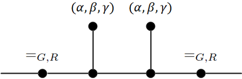
Figure 1: A binary gadget.

We calculate its signature $S$ as follows: It will be the matrix product of 4 matrices. The first matrix is $(=_{G,R})=\begin{bmatrix}0&0&0\\ 0&1&0\\ 0&0&1\end{bmatrix}$. The second is the matrix form $M$ of $\langle\mathbf{u},\mathbf{F}\rangle$, where $\mathbf{u}=(\alpha,\beta,\gamma)$, and we get

		$\alpha g+\beta y+\gamma w$
	$\alpha y+\beta x$		$\alpha w+\gamma z$
$\alpha x+\beta a$		$0$		$\alpha z+\gamma b$

Thus the matrix form is

$$M=\begin{bmatrix}\alpha g+\beta y+\gamma w&\alpha y+\beta x&\alpha w+\gamma z\\ \alpha y+\beta x&\alpha x+\beta a&0\\ \alpha w+\gamma z&0&\alpha z+\gamma b\end{bmatrix}.$$

The third matrix will be $M$ as well, and we note that $M$ is symmetric, $M^{\tt T}=M$. The fourth will be $=_{G,R}$ again, which is also symmetric. We can calculate the $2\times 2$ matrix for the signature $S^{*\rightarrow\{G,R\}}$ as a function on the restricted domain $\{G,R\}$ to be $\begin{bmatrix}0&1&0\\ 0&0&1\end{bmatrix}MM^{\tt T}\begin{bmatrix}0&0\\ 1&0\\ 0&1\end{bmatrix}$. Thus the signature $S^{*\rightarrow\{G,R\}}$ can be computed as follows, picking only the second and third rows of $M$:

$$\begin{bmatrix}\alpha y+\beta x&\alpha x+\beta a&0\\ \alpha w+\gamma z&0&\alpha z+\gamma b\end{bmatrix}\begin{bmatrix}\alpha y+\beta x&\alpha w+\gamma z\\ \alpha x+\beta a&0\\ 0&\alpha z+\gamma b\end{bmatrix}.$$

Written in the symmetric signature notation on domain size 2 we have

$$[(\alpha y+\beta x)^{2}+(\alpha x+\beta a)^{2},(\alpha y+\beta x)(\alpha w+\gamma z),(\alpha w+\gamma z)^{2}+(\alpha z+\gamma b)^{2}].$$ (5)

2.5 Symmetry and Decomposition

We say a function is decomposable, if it has arity at least $2$, and is a product of two functions (of arity at least $1$) applied to its two disjoint variable subsets respectively.

Fact 2.

If a symmetric function $\mathbf{F}=\mathbf{A}(x_{1})\mathbf{B}(x_{2},\cdots,x_{r})$, then there is a constant $c$, such that $\mathbf{F}=c\prod_{i=1}^{r}\mathbf{A}(x_{i})$.

Proof.

If $\mathbf{A}\equiv 0$ then it is trivial. We can assume $\mathbf{A}(a)\neq 0$.

If $r=2$, then by $\mathbf{F}=\mathbf{A}\mathbf{B}$, $\mathbf{A}(a)\mathbf{B}(x_{2})=\mathbf{A}(x_{2})\mathbf{B}(a)$. Hence, $\mathbf{A}(a)\mathbf{F}=\mathbf{A}(a)\mathbf{A}(x_{1})\mathbf{B}(x_{2})=\mathbf{B}(a)\mathbf{A}(x_{1})\mathbf{A}(x_{2})$, and we can set $c=\mathbf{A}(a)^{-1}\mathbf{B}(a)$.

If $r>2$, restricting to $x_{1}=a$, we see that $\mathbf{B}$ is symmetric. From $\mathbf{F}=\mathbf{A}(x_{1})\mathbf{B}(x_{2},\ldots,x_{r})$, we get $\mathbf{A}(a)\mathbf{B}(x_{2},\ldots,x_{r})=\mathbf{A}(x_{2})\mathbf{B}(a,x_{3},\ldots,x_{r})$. This means that $\mathbf{B}(x_{2},\ldots,x_{r})$ is a product of $\mathbf{A}(x_{2})$ and a function on $(x_{3},\ldots,x_{r})$. By induction hypothesis, the conclusion holds. ∎

For the general case, the idea is similar. If a symmetric $F$ is decomposed into $\mathbf{A}$ and $\mathbf{B}$, we utilize this to cut $\mathbf{A}$ and $\mathbf{B}$ into smaller pieces.

Fact 3.

If a symmetric function $\mathbf{F}=\mathbf{A}(x_{1}\cdots,x_{r})\mathbf{B}(x_{r+1},\cdots,x_{r+s})$, that is, it is decomposable, then for some constant $c$, and unary function $C$, $\mathbf{F}=c\prod_{i=1}^{r+s}\mathbf{C}(x_{i})$.

Proof.

For convenience we write $(y_{1},\cdots,y_{s})=(x_{r+1},\cdots,x_{r+s})$. If $r=1$ or $s=1$, we are done by Fact 2. Let $r>1$ and $s>1$. If $\mathbf{A}\equiv 0$ it is done. We can assume $\mathbf{A}(a_{1},\cdots,a_{r})\neq 0$.

By symmetry, we get $\mathbf{A}(a_{1},\cdots,a_{r})\mathbf{B}(y_{1},\cdots,y_{s})=\mathbf{A}(y_{1},a_{2},\cdots,a_{r})\mathbf{B}(a_{1},y_{2}\cdots,y_{s})$. Thus $\mathbf{B}$ satisfies the assumption of Fact 2. So $\mathbf{B}(y_{1},\cdots,y_{s})$ has the form $c^{\prime}\prod_{j=1}^{s}\mathbf{C}(y_{j})$. Then $\mathbf{F}$ has the form $\mathbf{C}(y_{1})(c^{\prime}\mathbf{A}(x_{1}\cdots,x_{r})\prod_{j=2}^{s}\mathbf{C}(y_{j}))$. By Fact 2 again, we get the conclusion.

∎

By Fact 3, if a symmetric function is decomposable, then it is a tensor power of a unary function. It is in $\langle\mathcal{U}\rangle-\mathcal{U}$, and degenerate.

We have seen symmetry can help to decompose a decomposable function into smaller parts. Next fact shows that some “partial symmetry” property also helps.

Fact 4.

Suppose $\mathbf{F}$ satisfies $\mathbf{F}(x_{1},x_{2},y_{1},y_{2})=\mathbf{F}(x_{2},x_{1},y_{1},y_{2})=\mathbf{F}(x_{1},x_{2},y_{2},y_{1})$. If $\mathbf{F}=\mathbf{A}(x_{1})\mathbf{B}(x_{2},y_{1},y_{2})$, then there are binary functions $C,D$, such that $\mathbf{F}=\mathbf{C}(x_{1},x_{2})\mathbf{D}(y_{1},y_{2})$.

The proof is similar to Facts 2 and 3.

Fact 5.

Suppose $\mathbf{F}$ satisfies $\mathbf{F}(x_{1},x_{2},y_{1},y_{2})=\mathbf{F}(x_{2},x_{1},y_{1},y_{2})=\mathbf{F}(x_{1},x_{2},y_{2},y_{1})$. If $\mathbf{F}$ is decomposed into two binary functions, then there are binary functions $\mathbf{A},\mathbf{B}$, either $\mathbf{F}=\mathbf{A}(x_{1},x_{2})\mathbf{B}(y_{1},y_{2})$ or $\mathbf{F}=\mathbf{A}(x_{1},y_{1})\mathbf{B}(x_{2},y_{2})$.

The proof is straightforward. If $\mathbf{F}$ is decomposed into two binary functions of other forms, just utilize the “partial symmetry” property to rotate it into one of the two forms.

In our hardness proofs, we will need to use some gadget with this “partial symmetry” property to realize a function $\mathbf{F}$ of arity 4 that can not be decomposed into two binary functions ($\mathbf{F}\not\in\langle\mathcal{T}\rangle$). By Fact 5, we only need to show that it cannot be decomposed into these two forms. We will call this the partial symmetry argument .

2.6 Known Dichotomy Theorems

We say a function set $\mathcal{F}$ is closed under tensor product, if for any $\mathbf{A},\mathbf{B}\in\mathcal{F}$, $\mathbf{A}\otimes\mathbf{B}\in\mathcal{F}$. Tensor closure $\langle\mathcal{F}\rangle$ of a set $\mathcal{F}$ is the minimum set containing $\mathcal{F}$, closed under tensor product. This closure clearly exists, being the set of all functions obtained by performing a finite sequence of tensor products from $\mathcal{F}$.

We use $\mathcal{U}$ to denote the set of all unary functions. $\mathcal{E}$ is the set of all functions $F$ such that $F$ is zero except on two inputs $(a_{1},\ldots,a_{n})$ and $(\bar{a}_{1},\ldots,\bar{a}_{n})=(1-a_{1},\ldots,1-a_{n})$. In other words, $F\in\mathcal{E}$ iff its support is contained in a pair of complementary points. We think of $\mathcal{E}$ as a generalized form of Equality function. Equivalently, these are obtained by connecting some subset of variables of Equality with binary Disequality $\not=_{2}$. We use $\mathcal{M}$ to denote the set of all functions $F$ such that $F$ is zero except on $n+1$ inputs whose Hamming weight is at most $1$, where $n$ is the arity of $F$. The name $\mathcal{M}$ is given for matching. Finally $\mathcal{T}$ is the set of all functions of arity at most $2$. Note that $\mathcal{U}$ is a subset of $\mathcal{E}$, $\mathcal{M}$ and $\mathcal{T}$.

Suppose $\mathcal{F}$ is a function set and $M$ is a $2\times 2$ matrix. We use $M\mathcal{F}$ to denote the set $\{M^{\otimes r_{F}}F|F\in\mathcal{F},r_{F}={\rm arity}(F)\}$, the set consisting of all functions in $\mathcal{F}$ transformed by a matrix $M$. $Z_{1}=\left(\begin{array}[]{cc}1&1\\ i&-i\end{array}\right)$ and $Z_{2}=\left(\begin{array}[]{cc}1&1\\ -i&i\end{array}\right)$. Note that $Z_{1}\mathcal{E}=Z_{2}\mathcal{E}$.

Theorem 2.4.

[16] Let $\mathcal{F}$ be any set of complex valued functions in Boolean variables. The problem Holant${}^{*}(\mathcal{F})$ is polynomial time computable, if

1. $\mathcal{F}\subseteq\langle\mathcal{T}\rangle$, or

2. for some orthogonal matrix $H$, $\mathcal{F}\subseteq\langle H\mathcal{E}\rangle$, or

3. $\mathcal{F}\subseteq\langle Z_{1}\mathcal{E}\rangle$, or

4. for some $Z\in\{Z_{1},Z_{2}\}$, $\mathcal{F}\subseteq\langle Z\mathcal{M}\rangle$.

In all other cases, Holant${}^{*}(\mathcal{F})$ is #P-hard.

This theorem is a generalization to not necessarily symmetric function sets from the following theorem which only applies to symmetric function sets. It is also very conceptual; however the following theorem is very easy to apply.

Theorem 2.5.

[14] Let ${\cal F}$ be any set of non-degenerate, symmetric, complex-valued signatures in Boolean variables. If ${\cal F}$ is of one of the following types, then ${\rm Holant}^{*}({\cal F})$ is in P, otherwise it is #P-hard.

1. Any signature in ${\cal F}$ is of arity at most 2;

2. There exist two constants $a$ and $b$ ($b\neq\pm 2ia$, depending only on ${\cal F}$), such that for all signatures $[f_{0},f_{1},\ldots,f_{n}]$ in ${\cal F}$ one of the two conditions is satisfied: (1) for every $k=0,1,\ldots,n-2$, we have $af_{k}+bf_{k+1}-af_{k+2}=0$; (2) $n=2$ and the signature $[f_{0},f_{1},f_{2}]$ is of the form $[2a\lambda,b\lambda,-2a\lambda]$.

3. For every signature $[f_{0},f_{1},\ldots,f_{n}]\in{\cal F}$ one of the two conditions is satisfied: (1) For every $k=0,1,\ldots,n-2$, we have $f_{k}+f_{k+2}=0$; (2) $n=2$ and the signature $[f_{0},f_{1},f_{2}]$ is of the form $[\lambda,0,\lambda]$.

4. There exists $\alpha\in\{2i,-2i\}$, such that for any signature $f\in\mathcal{F}$ of arity $n$, for $0\leq k\leq n-2$, we have $f_{k+2}=\alpha f_{k+1}+f_{k}$.

In Holant^∗ problems, unary functions are freely available. There is no difference between Holant${}^{*}(\mathcal{F}-\langle\mathcal{U}\rangle)$ and Holant${}^{*}(\mathcal{F}\cup\langle\mathcal{U}\rangle)$. Theorem 2.5 is stated for $\mathcal{F}-\langle\mathcal{U}\rangle$.

We give the correspondence between Theorem 2.4 and 2.5. Consider the symmetric subset of the first tractable class $\langle\mathcal{T}\rangle$ in Theorem 2.4. If a symmetric function in $\langle\mathcal{T}\rangle$ has arity larger than 2, it is decomposable and degenerate.

The function sets in Theorem 2.5 in forms 2 to 4 can be described by,

$$\mathcal{P}_{a,b}=\{[f_{0},f_{1},\cdots,f_{n}]|n\in\mathbb{N},ax_{k}+bx_{k+1}-ax_{k+2}=0\}\cup\{\lambda[2a,b,-2a]\mid\lambda\in\mathbb{C}\},$$ (6)

$$\mathcal{P}=\{[f_{0},f_{1},\cdots,f_{n}]|n\in\mathbb{N},f_{k}+f_{k+2}=0\}\cup\{\lambda[1,0,1]\mid\lambda\in\mathbb{C}\}.$$

Form 2 and 4 are described by $\mathcal{P}_{a,b}$ with $(a,b)$ not both zero, with Form 4 corresponding to $\mathcal{P}_{1,\pm 2i}$. Form 3 is described by $\mathcal{P}$. Note that for $\alpha=\pm 2i$, a binary $f$ with $f_{2}=\alpha f_{1}+f_{0}$ is degenerate. In $\mathcal{P}_{a,b}$, we always require $(a,b)\neq(0,0)$, and $(a,b)$ is equivalent to any non-zero multiple of it. When we say all $\mathcal{P}_{a,b}$, we let $(a,b)$ range over all $\mathbb{C}^{2}-\{(0,0)\}$ (equivalently the projective line $\mathbb{P}_{\mathbb{C}}^{1}$).

By Fact 3 a non-degenerate symmetric function must not be decomposable. It is in a set of tractable case $j$ in Theorem 2.4, iff it is in the corresponding set of tractable case $j$ in Theorem 2.5. For example, suppose $H=\left(\begin{array}[]{cc}u&v\\ s&t\end{array}\right)$ is an orthogonal matrix. $H\mathcal{E}$ corresponds to the set $\mathcal{P}_{a,b}$, where the corresponding relation is that 3 vectors $(u^{2},us,s^{2}),(v^{2},vt,t^{2}),(a,b,-a)$ form an orthogonal independent vector set. One $\mathcal{P}_{a,b}$ corresponds to two $(H\mathcal{E})^{S}$, given by $H$ and $H\tau$, where $\tau=\left(\begin{array}[]{cc}0&1\\ 1&0\end{array}\right)$ exchanges the two columns of $H$.

2.7 Polynomial Argument

Fact 6.

The product of two non-zero polynomials is a non-zero polynomial.

It is a simple fact that a polynomial ring (in any number of indeterminants and over any field) is an integral domain, and thus has no zero divisor. The way we will use this fact is as follows. When we design some gadget, usually there are some unary functions $(\alpha,\beta,\gamma)$ in this gadget, which work as parameters in order for the signature realized by the gadget to satisfy some conditions (for example, it should have full rank). Usually a condition can be described by a polynomial $P(\alpha,\beta,\gamma)$ in these parameters, such that when $P(\alpha_{0},\beta_{0},\gamma_{0})\neq 0$, the signature realized by the gadget using the unary function $(\alpha_{0},\beta_{0},\gamma_{0})$ satisfies this condition.

By Fact 6, when there are several such conditions to satisfy, we only need to show each polynomial $P_{i}$ is not zero, usually by finding some point $(\alpha_{i},\beta_{i},\gamma_{i})$ for each $P_{i}$. This guarantees the existence of some common parameter value $(\alpha^{*},\beta^{*},\gamma^{*})$ such that $\prod_{i}P_{i}(\alpha^{*},\beta^{*},\gamma^{*})\not=0$. The value $(\alpha^{*},\beta^{*},\gamma^{*})$ is implicit and not important; it has no direct connection to the choice of each $(\alpha_{i},\beta_{i},\gamma_{i})$. This method is already used in [16]. In proof, we quote it as the polynomial argument .

3 Statement of the Dichotomy Theorem

Theorem 3.1.

Let $\mathbf{F}$ be a symmetric ternary function over domain $\{B,G,R\}$. Then Holant${}^{*}(\mathbf{F})$ is #P-hard unless $\mathbf{F}$ is of one of the following three forms, in which case the problem is in polynomial time.

1. There exist three vectors $\alpha$, $\beta$, and $\gamma$ of dimension 3 such that they are mutually orthogonal to each other, i.e. $\langle\mbox{\boldmath$\alpha$, $\beta$}\rangle=0$, $\langle\mbox{\boldmath$\alpha$, $\gamma$}\rangle=0$ and $\langle\mbox{\boldmath$\beta$, $\gamma$}\rangle=0$, and

   $$\mathbf{F}=\mbox{\boldmath$\alpha$}^{\otimes 3}+\mbox{\boldmath$\beta$}^{\otimes 3}+\mbox{\boldmath$\gamma$}^{\otimes 3};$$

2. There exist three vectors $\alpha$, $\beta_{1}$, and $\beta_{2}$ of dimension 3 such that $\langle\mbox{\boldmath$\alpha$, $\beta_{1}$}\rangle=0$, $\langle\mbox{\boldmath$\alpha$, $\beta_{2}$}\rangle=0$, $\langle\mbox{\boldmath$\beta_{1}$, $\beta_{1}$}\rangle=0$, $\langle\mbox{\boldmath$\beta_{2}$, $\beta_{2}$}\rangle=0$ and

   $$\mathbf{F}=\mbox{\boldmath$\alpha$}^{\otimes 3}+\mbox{\boldmath$\beta_{1}$}^{\otimes 3}+\mbox{\boldmath$\beta_{2}$}^{\otimes 3};$$

3. There exist two vectors $\beta$ and $\gamma$ of dimension 3 and a function ${\mathbf{F}}_{\beta}$ of arity three, such that $\mbox{\boldmath$\beta$}\neq\mathbf{0}$, $\langle\mbox{\boldmath$\beta$, $\beta$}\rangle=0$, $\langle\mathbf{F}_{\beta},\mbox{\boldmath$\beta$}\rangle=\mathbf{0}$ and

   $$\mathbf{F}=\mathbf{F}_{\bf\beta}+\mbox{\boldmath$\beta$}^{\otimes 2}\otimes\mbox{\boldmath$\gamma$}+\mbox{\boldmath$\beta$}\otimes\mbox{\boldmath$\gamma$}\otimes\mbox{\boldmath$\beta$}+\mbox{\boldmath$\gamma$}\otimes\mbox{\boldmath$\beta$}^{\otimes 2}.$$

Remarks: 1. In the forms above, the vectors $\alpha$, $\beta$, $\gamma$, $\beta_{1}$, $\beta_{2}$ can be the zero vector (except $\beta$ in form 3.)
2. In form 3, $\mathbf{F}$ is the sum of $\mathbf{F}_{\beta}$ with ($1/2$ of) the symmetrization of $\mbox{\boldmath$\beta$}^{\otimes 2}\otimes\mbox{\boldmath$\gamma$}$. The constant factor $1/2$ doesn’t matter, and can be absorbed in $\gamma$.
3. Let $T$ be an orthogonal $3\times 3$ matrix, then $\mathbf{F}$ is of one of the three forms above iff $T^{\otimes 3}\mathbf{F}$ is.

3.1 Canonical Forms for Tractable Cases

Theorem 3.1 gives a complete list of tractable cases for Holant${}^{*}(\mathbf{F})$. Before we give the proof of tractability we need to discuss these tractable forms in some detail, and give various canonical forms of these tractable cases, under an orthogonal transformation $T$. We note that for an orthogonal $T$, the arity 2 Equality gate $(=_{2})$ (on any domain size) is invariant, the unary signatures are transformed to unary signatures, and the formal description of the three forms of $\mathbf{F}$ is also invariant, i.e., $\mathbf{F}$ is of one of the three forms iff $T^{\otimes 3}\mathbf{F}$ is.

In terms of the canonical forms, Theorem 3.1 can be restated as follows. We will write $T\mathbf{F}$ for $T^{\otimes 3}\mathbf{F}$ for simplicity.

Theorem 3.2.

Let $\mathbf{F}$ be a symmetric ternary function over domain $\{B,G,R\}$. Then Holant${}^{*}(\mathbf{F})$ is #P-hard unless under an orthogonal transformation $T$, the function $T\mathbf{F}$ is of one of the following forms, in which case the problem is in P.

1. For some $a,b,c\in\mathbb{C}$,

   $$T\mathbf{F}=a\mbox{\boldmath$e_{1}$}^{\otimes 3}+b\mbox{\boldmath$e_{2}$}^{\otimes 3}+c\mbox{\boldmath$e_{3}$}^{\otimes 3}.$$

2. For some $c\not=0$ and $\lambda\in\mathbb{C}$,

   $$cT\mathbf{F}=\mbox{\boldmath$\beta_{0}$}^{\otimes 3}+\overline{\mbox{\boldmath$\beta_{0}$}}^{\otimes 3}+\lambda\mbox{\boldmath$e_{3}$}^{\otimes 3},$$

   where $\mbox{\boldmath$\beta_{0}$}=\frac{1}{\sqrt{2}}(1,i,0)^{\tt T}$, and $\overline{\mbox{\boldmath$\beta_{0}$}}$ is its conjugate $\frac{1}{\sqrt{2}}(1,-i,0)^{\tt T}$.

3. For $\epsilon\in\{0,1\}$,

   $$T\mathbf{F}=\mathbf{F}_{0}+\epsilon\rm{Sym}(\mbox{\boldmath$\beta_{0}$}\otimes\mbox{\boldmath$\beta_{0}$}\otimes\overline{\mbox{\boldmath$\beta_{0}$}}),$$

   where $\mathbf{F}_{0}$ satisfies the annihilation condition $\langle\mathbf{F}_{0},\mbox{\boldmath$\beta_{0}$}\rangle=\mathbf{0}.$

We start by defining the complex version of rotations. For any $z\in\mathbb{C}$, let $c=\cos z=\frac{e^{iz}+e^{-iz}}{2}$ and $s=\sin z=\frac{e^{iz}-e^{-iz}}{2i}$, and $T_{2}=\begin{bmatrix}c&s\\ -s&c\end{bmatrix}$. Then $c^{2}+s^{2}=1$ and $T_{2}$ is a $2\times 2$ orthogonal matrix. If $\begin{bmatrix}a\\ b\end{bmatrix}\in\mathbb{C}^{2}$ is not isotropic, then $T_{2}\begin{bmatrix}a\\ b\end{bmatrix}=\begin{bmatrix}ca+sb\\ -sa+cb\end{bmatrix}$ is also not isotropic $(ca+sb)^{2}+(-sa+cb)^{2}=a^{2}+b^{2}\not=0$. Let $\eta=\cot z=i\frac{e^{iz}+e^{-iz}}{e^{iz}-e^{-iz}}=i\frac{e^{2iz}+1}{e^{2iz}-1}$, we want a suitable $z\in\mathbb{C}$, such that $-sa+cb=0$. The Möbius map $\xi\mapsto i\frac{\xi+1}{\xi-1}$ is a one-to-one onto map on the extended Riemann complex plane $\mathbb{C}\cup\{\infty\}$. As $z\mapsto e^{2z}$ maps $\mathbb{C}$ onto $\mathbb{C}-\{0\}$, the mapping $z\mapsto\eta=\cot z$ from $\mathbb{C}$ has image $\mathbb{C}\cup\{\infty\}-\{i,-i\}$. This proves that we can find an orthogonal $T_{2}$ such that $T_{2}\begin{bmatrix}a\\ b\end{bmatrix}=\begin{bmatrix}a^{\prime}\\ 0\end{bmatrix}$, where $a^{\prime 2}=a^{2}+b^{2}$, for any non-isotropic $\begin{bmatrix}a\\ b\end{bmatrix}$.

Suppose $v=(a_{1},a_{2},\ldots,a_{d})^{\tt T}\in\mathbb{C}^{d}$ is non-isotropic, $d\geq 2$. Suppose $d^{\prime}$ is the number of non-zero entries $a_{i}$. Then $d^{\prime}\geq 1$. By a permutation matrix (which is orthogonal) we may assume they are $a_{1},\ldots,a_{d^{\prime}}$. Suppose $d^{\prime}\geq 2$. There exist $1\leq i<j\leq d^{\prime}$, such that $(a_{i},a_{j})^{\tt T}$ is non-isotropic. Otherwise, summing $a_{i}^{2}+a_{j}^{2}$ over all distinct pairs $(i,j)$ among the non-zero entries $1\leq i<j\leq d^{\prime}$ we get $(d^{\prime}-1)\sum_{i=1}^{d^{\prime}}a_{i}^{2}=0$ and $v$ is isotropic. Hence, we can use a permutation matrix (which is orthogonal) to map $v$ such that $a_{1}^{2}+a_{2}^{2}\not=0$. By a rotation described above, we may use an orthogonal matrix of the form ${\rm diag}(T_{2},I_{d-2})$ to transform $v$, such that it has one fewer non-zero entries but with the same value $\langle v,v\rangle=\sum_{i=1}^{d}a_{i}^{2}$. By induction, we have proved

Lemma 3.3.

For any non-isotropic $v=(a_{1},a_{2},\ldots,a_{d})^{\tt T}\in\mathbb{C}^{d}$, $d\geq 1$, there exists an orthogonal matrix $T$ such that $Tv=(\pm\sqrt{\langle v,v\rangle},0,\ldots,0)^{\tt T}$. (Both $\pm$ are feasible.)

Now suppose $v\in\mathbb{C}^{d}$ is a non-zero isotropic vector. Certainly $d\geq 2$. We want to show that there is an orthogonal matrix $T$ transforming $v$ to $\mbox{\boldmath$\beta_{0}$}=\frac{1}{\sqrt{2}}(1,i,0,\ldots,0)^{\tt T}$. First suppose $d=2$. Then $v=(a,b)^{\tt T}$ and $b=\pm ai$, and $v=a\begin{bmatrix}1\\ \pm i\end{bmatrix}$. As $v\not=0$, we have $a\not=0$. We may use $\begin{bmatrix}1&0\\ 0&-1\end{bmatrix}$, to get $v=a\begin{bmatrix}1\\ i\end{bmatrix}$. Use a complex rotation $T_{2}$ defined above we get $T_{2}v=a\begin{bmatrix}c+si\\ -s+ci\end{bmatrix}=a(c+si)\begin{bmatrix}1\\ i\end{bmatrix}$. As $c+si=e^{iz}$ can be an arbitrary nonzero complex number, we may choose $z$ such that $e^{iz}=\frac{1}{\sqrt{2}a}$. This gives us $T_{2}v=\frac{1}{\sqrt{2}}\begin{bmatrix}1\\ i\end{bmatrix}$. It is clear that we could also go to any non-zero multiple of $\begin{bmatrix}1\\ i\end{bmatrix}$, as well as $\begin{bmatrix}1\\ -i\end{bmatrix}$.

Now suppose $d>2$. Let $v=(a_{1},a_{2},\ldots,a_{d})^{\tt T}\not=0$ be isotropic. If $a_{1}=0$, then $(a_{2},\ldots,a_{d})^{\tt T}\not=0$ is isotropic. By induction there exists an order $d-1$ orthogonal matrix $T^{\prime}$ such that ${\rm diag}(1,T^{\prime})v=\frac{1}{\sqrt{2}}(0,1,i,0,\ldots,0)^{\tt T}$. Then we complete the induction by a permutation matrix, obtaining an order $d$ orthogonal matrix $T$ such that $Tv=\mbox{\boldmath$\beta_{0}$}$. Next we assume $a_{1}\not=0$. Then $v^{\prime}=(a_{2},\ldots,a_{d})^{\tt T}$ is not isotropic and non-zero. By Lemma 3.3, there exists an order $d-1$ orthogonal matrix $T^{\prime}$ such that ${\rm diag}(1,T^{\prime})v=(a_{1},\sqrt{\langle v^{\prime},v^{\prime}\rangle},0,\ldots,0)^{\tt T}$. Since $v$ is isotropic, we have $\sqrt{\langle v^{\prime},v^{\prime}\rangle}=\pm a_{1}i$. So we have ${\rm diag}(1,T^{\prime})v=a_{1}(1,\pm i,0,\ldots,0)^{\tt T}$. And by the above discussion we get an orthogonal $T$ such that $Tv=\mbox{\boldmath$\beta_{0}$}$. We have proved

Lemma 3.4.

For any non-zero isotropic $v=(a_{1},a_{2},\ldots,a_{d})^{\tt T}\in\mathbb{C}^{d}$, $d\geq 2$, there exists an orthogonal matrix $T$ such that $Tv=\mbox{\boldmath$\beta_{0}$}=\frac{1}{\sqrt{2}}(1,i,0,\ldots,0)^{\tt T}$. (Both $(1,i,0,\ldots,0)^{\tt T}$ and $(1,-i,0,\ldots,0)^{\tt T}$, and all non-zero multiples of them are feasible.)

Now set $d=3$. Our next task is to describe the set of all order 3 orthogonal matrices $T$ which fixes $\beta_{0}$.

Let the first two columns of $T$ be denoted by $u=(a_{1},a_{2},a_{3})^{\tt T}$ and $v=(b_{1},b_{2},b_{3})^{\tt T}$. We can derive $a_{1}=1-a_{2}i$, $b_{1}=a_{2}$, $b_{2}=1+a_{2}i$, and $a_{3}=-b_{3}i$. It follows that the first two columns are of the form $\begin{bmatrix}1-ix&x\\ x&1+ix\\ iy&-y\end{bmatrix}$. Moreover, the columns are unit vectors, and so $x=iy^{2}/2$. If we form the cross-product of these two vectors, we obtain $(-iy,y,1)^{\tt T}$. This and its negation $(iy,-y,-1)^{\tt T}$ can be the third column vector of $T$. Thus the orthogonal matrix $T$ has the form

$$T=\begin{bmatrix}1+y^{2}/2&iy^{2}/2&iy\\ iy^{2}/2&1-y^{2}/2&-y\\ iy&-y&-1\end{bmatrix},$$ (7)

or changing the last column to its negative. This is a complete description of the set of $3\times 3$ orthogonal matrices $T$ such that $T\mbox{\boldmath$\beta_{0}$}=\mbox{\boldmath$\beta_{0}$}$.

Our next task is to determine what canonical form a vector $v$ can take, under the mapping of such an orthogonal matrix $T$ which fixes $\beta_{0}$. First we prove a simple lemma.

Lemma 3.5.

If $\mathbf{\beta}_{1},\mathbf{\beta}_{2}\in\mathbb{C}^{3}$ are isotropic, and linearly independent. Then $\langle\mathbf{\beta}_{1},\mathbf{\beta}_{2}\rangle\not=0$, and there exists an orthogonal matrix $T$ such that $T\mathbf{\beta}_{1}=\mbox{\boldmath$\beta_{0}$}$ and $T\mathbf{\beta}_{2}=\langle\mathbf{\beta}_{1},\mathbf{\beta}_{2}\rangle\overline{\mbox{\boldmath$\beta_{0}$}}$. Let $\lambda=1/\sqrt{\langle\mathbf{\beta}_{1},\mathbf{\beta}_{2}\rangle}$, there exists an orthogonal matrix $T$ such that $\lambda T\mathbf{\beta}_{1}=\mbox{\boldmath$\beta_{0}$}$ and $\lambda T\mathbf{\beta}_{2}=\overline{\mbox{\boldmath$\beta_{0}$}}$.

Proof.

By Lemma 3.4, we have an orthogonal $T_{1}$, such that $T_{1}\mathbf{\beta}_{1}=\mbox{\boldmath$\beta_{0}$}$. Let $\mathbf{\gamma}=T_{1}\mathbf{\beta}_{2}$. Write $\mathbf{\gamma}=\begin{bmatrix}a\\ b\\ c\end{bmatrix}$. If $\langle\mathbf{\beta}_{1},\mathbf{\beta}_{2}\rangle=0$, then, since $T_{1}$ preserves inner product, $a+bi=0$ and $c^{2}=-(a^{2}+b^{2})=0$. Hence, $\mathbf{\gamma}$ is linearly dependent on $\beta_{0}$, and thus $\mathbf{\beta}_{2}$ is linearly dependent on $\mathbf{\beta}_{1}$, a contradiction. Hence $\langle\mathbf{\beta}_{1},\mathbf{\beta}_{2}\rangle\not=0$.

Now we may as well assume the given vectors are $\beta_{0}$ and $\mathbf{\gamma}$. Consider those orthogonal matrices $T$ in (7) fixing $\beta_{0}$. Let ${u}=\mathbf{\gamma}/\langle{\mathbf{\gamma}},{\mbox{\boldmath$\beta_{0}$}}\rangle$. Then $\langle u,{\mbox{\boldmath$\beta_{0}$}}\rangle=1$. We want a $T$ such that $T\overline{\mbox{\boldmath$\beta_{0}$}}={u}$. Write ${v}=\frac{1}{\sqrt{2}}{u}=\begin{bmatrix}a\\ b\\ c\end{bmatrix}$, then $\langle{v},(1,i,0)^{\tt T}\rangle=\langle{u},\mbox{\boldmath$\beta_{0}$}\rangle=1$, and it follows that $a+bi=1$ and so $-c^{2}=a^{2}+b^{2}=1-2bi$. Hence ${v}=(\frac{1-c^{2}}{2},\frac{1+c^{2}}{2i},c)^{\tt T}$. On the other hand, from (7), $T(1,-i,0)^{\tt T}=(1+y^{2},(1-y^{2})/i,2yi)^{\tt T}$. Then by setting $y=c/i$ we get $T(1,-i,0)^{\tt T}=2{v}$. Hence $T\overline{\mbox{\boldmath$\beta_{0}$}}=\frac{1}{\sqrt{2}}T(1,-i,0)^{\tt T}=\sqrt{2}{v}={u}$.

The last conclusion of Lemma 3.5 follows from what has been proved applied to the pair $\lambda\mathbf{\beta}_{1}$ and $\lambda\mathbf{\beta}_{2}$. ∎

Lemma 3.6.

Suppose $\mathbf{\beta}\in\mathbb{C}^{3}$ is isotropic, $\mathbf{\gamma}\in\mathbb{C}^{3}$ is not isotropic, $\{\mathbf{\beta},\mathbf{\gamma}\}$ are linearly independent, and $\langle\mathbf{\beta},\mathbf{\gamma}\rangle=0$. Then there exists an orthogonal matrix $T$ such that $T\mathbf{\beta}=\mbox{\boldmath$\beta_{0}$}$ and $T\mathbf{\gamma}=\sqrt{\langle\mathbf{\gamma},\mathbf{\gamma}\rangle}\mbox{\boldmath$e_{3}$}$. For $\lambda=1/\sqrt{\langle\mathbf{\gamma},\mathbf{\gamma}\rangle}$, there exists an orthogonal matrix $T$ such that $\lambda T\mathbf{\beta}=\mbox{\boldmath$\beta_{0}$}$ and $\lambda T\mathbf{\gamma}=\mbox{\boldmath$e_{3}$}$.

Proof.

By Lemma 3.4, we may assume $\mathbf{\beta}=\mbox{\boldmath$\beta_{0}$}$. Write $\lambda\mathbf{\gamma}=\begin{bmatrix}a\\ b\\ c\end{bmatrix}$. Then $a+bi=0$ and $c^{2}=a^{2}+b^{2}+c^{2}=1$. Depending on whether $c=\pm 1$, we use one of the two forms of $T$ in (7) fixing $\beta_{0}$. If $c=-1$, we set $y=-b$ in (7). If $c=+1$, we set $y=-b$ in the form of $T$ with the negated third column from (7).

The last conclusion follows from what has been proved applied to the pair $\lambda\mathbf{\beta}$ and $\lambda\mathbf{\gamma}$. ∎

We are now ready to address in what canonical form each of the three cases in Theorem 3.1 can take.

We consider each case in turn:

$\bullet$ There exist three vectors $\alpha$, $\beta$, and $\gamma$ of dimension 3 such that they are mutually orthogonal to each other, i.e. $\langle\mbox{\boldmath$\alpha$, $\beta$}\rangle=0$, $\langle\mbox{\boldmath$\alpha$, $\gamma$}\rangle=0$, $\langle\mbox{\boldmath$\beta$, $\gamma$}\rangle=0$, and

$$\mathbf{F}=\mbox{\boldmath$\alpha$}^{\otimes 3}+\mbox{\boldmath$\beta$}^{\otimes 3}+\mbox{\boldmath$\gamma$}^{\otimes 3}.$$

Let $r={\rm rank}\{\mbox{\boldmath$\alpha$, $\beta$, $\gamma$}\}$. If $r=0$, then $\mathbf{F}=\mathbf{0}$ is the identically zero function.

If $r=1$, and suppose $\mbox{\boldmath$\alpha$}\not=0$ and $\beta$ and $\gamma$ are linear multiples of $\alpha$. Then $\mathbf{F}=\mbox{\boldmath$\alpha^{\prime}$}^{\otimes 3}$ for some $\alpha^{\prime}$. Depending on whether $\alpha^{\prime}$ is isotropic, under an orthogonal transformation, $T\mathbf{F}$ takes the form

$$T\mathbf{F}=\mbox{\boldmath$\beta_{0}$}^{\otimes 3},~{}~{}~{}~{}\mbox{or}~{}~{}~{}~{}\lambda\mbox{\boldmath$e_{3}$}^{\otimes 3}.$$ (8)

Let $r=2$ and suppose $\alpha$ and $\beta$ are linearly independent. We show that without loss of generality we may assume $\mbox{\boldmath$\gamma$}=\mathbf{0}$. Let $\mbox{\boldmath$\gamma$}=a\mbox{\boldmath$\alpha$}+b\mbox{\boldmath$\beta$}$. Then $\langle\mbox{\boldmath$\gamma$},\mbox{\boldmath$\gamma$}\rangle=0$. If either $a=0$ or $b=0$, we can combine the term $\mbox{\boldmath$\gamma$}^{\otimes 3}$ with either $\mbox{\boldmath$\beta$}^{\otimes 3}$ or $\mbox{\boldmath$\alpha$}^{\otimes 3}$ respectively, and the term $\mbox{\boldmath$\gamma$}^{\otimes 3}$ disappears. If both $a,b\not=0$. By $\langle\mbox{\boldmath$\alpha$, $\beta$}\rangle=0$, $\langle\mbox{\boldmath$\alpha$, $\gamma$}\rangle=0$, $\langle\mbox{\boldmath$\beta$, $\gamma$}\rangle=0$, we get $a\langle\mbox{\boldmath$\alpha$, $\alpha$}\rangle=b\langle\mbox{\boldmath$\beta$, $\beta$}\rangle=0$. Hence $\langle\mbox{\boldmath$\alpha$, $\alpha$}\rangle=\langle\mbox{\boldmath$\beta$, $\beta$}\rangle=0$. This contradicts Lemma 3.5, by linear independence. Therefore in case $r=2$ we only need to consider $\mathbf{F}=\mbox{\boldmath$\alpha$}^{\otimes 3}+\mbox{\boldmath$\beta$}^{\otimes 3}$, and $\alpha$ and $\beta$ are linearly independent.

By Lemma 3.5 $\alpha$ and $\beta$ can not be both isotropic. Suppose one of them is isotropic. By Lemma 3.6, $\mathbf{F}$ takes the form

$$\mbox{\boldmath$\beta_{0}$}^{\otimes 3}+\lambda\mbox{\boldmath$e_{3}$}^{\otimes 3}$$ (9)

under an orthogonal transformation.

If $r=2$ and both $\alpha$ and $\beta$ are not isotropic, then there exists an orthogonal matrix $T$ such that $T\mbox{\boldmath$\alpha$}=\lambda\mbox{\boldmath$e_{1}$}$ and $T\mbox{\boldmath$\beta$}=\mu\mbox{\boldmath$e_{2}$}$, thus $\mathbf{F}$ takes the form

$$\lambda\mbox{\boldmath$e_{1}$}^{\otimes 3}+\mu\mbox{\boldmath$e_{2}$}^{\otimes 3}$$ (10)

under an orthogonal transformation.

Now suppose $r=3$. We claim none of $\alpha$, $\beta$, and $\gamma$ can be isotropic. Otherwise, say $\alpha$ is isotropic, then the linearly independent set $\{\mbox{\boldmath$\alpha$, $\beta$, $\gamma$}\}$ spans the conjugate vector $\overline{\mbox{\boldmath$\alpha$}}$. Then it follows that $\langle\mbox{\boldmath$\alpha$},\overline{\mbox{\boldmath$\alpha$}}\rangle=0$ and $\mbox{\boldmath$\alpha$}=\mathbf{0}$, a contradiction. Hence, under an orthogonal transformation $\mathbf{F}$ takes the form

$$\lambda\mbox{\boldmath$e_{1}$}^{\otimes 3}+\mu\mbox{\boldmath$e_{2}$}^{\otimes 3}+\nu\mbox{\boldmath$e_{3}$}^{\otimes 3}$$ (11)

$\bullet$ There exist three vectors $\alpha$, $\beta_{1}$, and $\beta_{2}$ of dimension 3 such that $\langle\mbox{\boldmath$\alpha$, $\beta_{1}$}\rangle=0$, $\langle\mbox{\boldmath$\alpha$, $\beta_{2}$}\rangle=0$, $\langle\mbox{\boldmath$\beta_{1}$, $\beta_{1}$}\rangle=0$, $\langle\mbox{\boldmath$\beta_{2}$, $\beta_{2}$}\rangle=0$ and

$$\mathbf{F}=\mbox{\boldmath$\alpha$}^{\otimes 3}+\mbox{\boldmath$\beta_{1}$}^{\otimes 3}+\mbox{\boldmath$\beta_{2}$}^{\otimes 3}.$$

Let $r={\rm rank}\{\mbox{\boldmath$\beta_{1}$},\mbox{\boldmath$\beta_{2}$}\}$. If $r=0$, then $\mathbf{F}=\mbox{\boldmath$\alpha$}^{\otimes 3}$. If $r=1$, we can combine the terms $\mbox{\boldmath$\beta_{1}$}^{\otimes 3}$ and $\mbox{\boldmath$\beta_{2}$}^{\otimes 3}$, and $\mathbf{F}$ takes the form $\mbox{\boldmath$\alpha$}^{\otimes 3}+\mbox{\boldmath$\beta^{\prime}$}^{\otimes 3}$, with $\langle\mbox{\boldmath$\alpha$},\mbox{\boldmath$\beta^{\prime}$}\rangle=0$. These cases have already been classified in the first form. $\mathbf{F}$ takes the forms in (8), (9) or (10).

Suppose $r=2$. By Lemma 3.5, for a suitable non-zero constant $\lambda=1/\sqrt{\langle\mbox{\boldmath$\beta_{1}$},\mbox{\boldmath$\beta_{2}$}\rangle}$, there exists an orthogonal matrix $T$ such that $\lambda T\mbox{\boldmath$\beta_{1}$}=\mbox{\boldmath$\beta_{0}$}$ and $\lambda T\mbox{\boldmath$\beta_{2}$}=\overline{\mbox{\boldmath$\beta_{0}$}}$. Under this transformation $\lambda T$, $\alpha$ is orthogonal to $e_{1}$ and $e_{2}$ which are in the linear span of $\beta_{0}$ and $\overline{\mbox{\boldmath$\beta_{0}$}}$. Hence $\alpha$ takes the form $c\mbox{\boldmath$e_{3}$}$.

We have proved that in this case, for some non-zero constant $\lambda$ and orthogonal matrix $T$,

$$\lambda T\mathbf{F}=\mbox{\boldmath$\beta_{0}$}^{\otimes 3}+\overline{\mbox{\boldmath$\beta_{0}$}}^{\otimes 3}+c\mbox{\boldmath$e_{3}$}^{\otimes 3}.$$ (12)

$\bullet$ There exist two vectors $\beta$ and $\gamma$ of dimension 3 and a (symmetric) function ${\mathbf{F}}_{\beta}$ of arity three, such that $\mbox{\boldmath$\beta$}\neq\mathbf{0}$, $\langle\mbox{\boldmath$\beta$, $\beta$}\rangle=0$, $\langle\mathbf{F}_{\beta},\mbox{\boldmath$\beta$}\rangle=\mathbf{0}$ and

$$\mathbf{F}=\mathbf{F}_{\beta}+\mbox{\boldmath$\beta$}^{\otimes 2}\otimes\mbox{\boldmath$\gamma$}+\mbox{\boldmath$\beta$}\otimes\mbox{\boldmath$\gamma$}\otimes\mbox{\boldmath$\beta$}+\mbox{\boldmath$\gamma$}\otimes\mbox{\boldmath$\beta$}^{\otimes 2}.$$

First we note that $\mbox{\boldmath$\beta$}^{\otimes 3}$ also satisfies the annihilation condition, $\langle\mathbf{F}_{\beta},\mbox{\boldmath$\beta$}\rangle=\mathbf{0}$, and can be combined to $\mathbf{F}_{\beta}$. Hence we can replace $\gamma$ by any $\mbox{\boldmath$\gamma$}+\lambda\mbox{\boldmath$\beta$}$.

There are the following cases, depending on whether $\langle\mbox{\boldmath$\beta$},\mbox{\boldmath$\gamma$}\rangle=0$ and whether $\gamma$ is isotropic.

Suppose $\langle\mbox{\boldmath$\beta$},\mbox{\boldmath$\gamma$}\rangle=0$. Then we can eliminate the terms $\mbox{\boldmath$\beta$}^{\otimes 2}\otimes\mbox{\boldmath$\gamma$}+\mbox{\boldmath$\beta$}\otimes\mbox{\boldmath$\gamma$}\otimes\mbox{\boldmath$\beta$}+\mbox{\boldmath$\gamma$}\otimes\mbox{\boldmath$\beta$}^{\otimes 2}$ by combining it to $\mathbf{F}_{\beta}$. We can transform $\beta$ to $\beta_{0}$. In this case, $\mathbf{F}$ takes the form

$$T\mathbf{F}=\mathbf{F}_{{\beta}_{0}}$$ (13)

where $\langle\mathbf{F}_{{\beta}_{0}},\mbox{\boldmath$\beta_{0}$}\rangle=\mathbf{0}$.

Suppose $\gamma$ is isotropic and $\langle\mbox{\boldmath$\beta$},\mbox{\boldmath$\gamma$}\rangle\not=0$. Then $\beta$ and $\gamma$ are linearly independent. By Lemma 3.5 there exists an orthogonal matrix $T$ such that

$$T\mathbf{F}=\mathbf{F}_{\mathbf{\beta}_{0}}+\lambda(\mbox{\boldmath$\beta_{0}$}^{\otimes 2}\otimes\overline{\mbox{\boldmath$\beta_{0}$}}+\mbox{\boldmath$\beta_{0}$}\otimes\overline{\mbox{\boldmath$\beta_{0}$}}\otimes\mbox{\boldmath$\beta_{0}$}+\overline{\mbox{\boldmath$\beta_{0}$}}\otimes\mbox{\boldmath$\beta_{0}$}^{\otimes 2}),$$

where $\lambda=\langle\mbox{\boldmath$\beta$},\mbox{\boldmath$\gamma$}\rangle\not=0$, and $\langle\mathbf{F}_{\beta_{0}},\mbox{\boldmath$\beta_{0}$}\rangle=0$. Let $T_{2}=\begin{bmatrix}c&s\\ -s&c\end{bmatrix}$, where $c=\cos z$ and $s=\sin z$. Then $T_{2}$ maps $\begin{bmatrix}1\\ i\end{bmatrix}$ to $(c+si)\begin{bmatrix}1\\ i\end{bmatrix}$ and maps $\begin{bmatrix}1\\ -i\end{bmatrix}$ to $(c-si)\begin{bmatrix}1\\ -i\end{bmatrix}$. To each term in

$$\mbox{\boldmath$\beta_{0}$}^{\otimes 2}\otimes\overline{\mbox{\boldmath$\beta_{0}$}}+\mbox{\boldmath$\beta_{0}$}\otimes\overline{\mbox{\boldmath$\beta_{0}$}}\otimes\mbox{\boldmath$\beta_{0}$}+\overline{\mbox{\boldmath$\beta_{0}$}}\otimes\mbox{\boldmath$\beta_{0}$}^{\otimes 2},$$

${\rm diag}(T_{2},1)^{\otimes 3}$ contributes a factor $(c+si)^{2}(c-si)=c+si=e^{z}$, which can be an arbitrarily chosen non-zero complex number. In particular we can set it to $1/\lambda$. Also note that ${\rm diag}(T_{2},1)^{\otimes 3}$ transforms $\mathbf{F}_{\beta_{0}}$ to another such function satisfying the annihilation condition $\langle\mathbf{F}_{\beta_{0}},\mbox{\boldmath$\beta_{0}$}\rangle=\mathbf{0}$. Thus we obtain the form of $\mathbf{F}$ under an orthogonal transformation

$$\mathbf{F}_{\beta_{0}}+\mbox{\boldmath$\beta_{0}$}^{\otimes 2}\otimes\overline{\mbox{\boldmath$\beta_{0}$}}+\mbox{\boldmath$\beta_{0}$}\otimes\overline{\mbox{\boldmath$\beta_{0}$}}\otimes\mbox{\boldmath$\beta_{0}$}+\overline{\mbox{\boldmath$\beta_{0}$}}\otimes\mbox{\boldmath$\beta_{0}$}^{\otimes 2}.$$ (14)

Suppose $\gamma$ is not isotropic and $\langle\mbox{\boldmath$\beta$},\mbox{\boldmath$\gamma$}\rangle\not=0$. Then we replace $\gamma$ by $\mbox{\boldmath$\gamma$}-c\mbox{\boldmath$\beta$}$, where $c=\langle\mbox{\boldmath$\gamma$},\mbox{\boldmath$\gamma$}\rangle/(2\langle\mbox{\boldmath$\beta$},\mbox{\boldmath$\gamma$}\rangle)$. Then $\mbox{\boldmath$\gamma$}-c\mbox{\boldmath$\beta$}$ is isotropic and we have reduced to the previous case.

Summarizing, we note that (8) and (9) are special cases of (13). (10) is a special case of (11). Then it is clear that Theorem 3.2 is equivalent to Theorem 3.1.

4 Tractability

Suppose $\mathbf{F}=[3;1,1;5,1,3;7,5,1,1]$. Is Holant${}^{*}(\mathbf{F})$ computable in polynomial time? It turns out that there are three pairwise orthogonal vectors $(1,-1,1)^{\tt T},(1,0,-1)^{\tt T}$ and $(1,2,1)^{\tt T}$ such that $\mathbf{F}={\scriptsize\begin{bmatrix}1\\ -1\\ 1\end{bmatrix}^{\otimes 3}+\begin{bmatrix}1\\ 0\\ -1\end{bmatrix}^{\otimes 3}+\begin{bmatrix}1\\ 2\\ 1\end{bmatrix}^{\otimes 3}}.$ By Theorem 3.1, Holant${}^{*}(\mathbf{F})$ is tractable. If we take $T=\frac{1}{\sqrt{6}}{\scriptsize\begin{bmatrix}\sqrt{2}&\sqrt{3}&1\\ -\sqrt{2}&0&2\\ \sqrt{2}&-\sqrt{3}&1\end{bmatrix}}$, then $T$ is orthogonal, and $\mathbf{F}=T^{\otimes 3}\mathbf{F}^{\prime}$, where $\mathbf{F}^{\prime}=\sqrt{27}\mbox{\boldmath$e_{1}$}^{\otimes 3}+\sqrt{8}\mbox{\boldmath$e_{2}$}^{\otimes 3}+\sqrt{216}\mbox{\boldmath$e_{3}$}^{\otimes 3}$. Hence we can perform an orthogonal transformation by $T$, then the problem Holant${}^{*}(\mathbf{F})$ is transformed to Holant${}^{*}(\mathbf{F}^{\prime})$. For $\mathbf{F}^{\prime}$ the polynomial time algorithm on any input graph $\Gamma$ is simple: In each connected component of $\Gamma$, any color from $\{B,G,R\}$ at a vertex $v$ uniquely determines the same color at all its neighbors, and the vertex contributes a factor $\sqrt{27}$ or $\sqrt{8}$ or $\sqrt{216}$ respectively. These values are multiplied over the connected component. Thus, if $G$ has connected components $C_{1},C_{2},\ldots,C_{k}$, and $C_{j}$ has $n_{j}$ vertices, then the Holant values is $\prod_{1\leq j\leq k}(\sqrt{27}^{n_{j}}+\sqrt{8}^{n_{j}}+\sqrt{216}^{n_{j}})$.

We believe for countless such questions, not only the problem is very natural, but also the answer is not obvious without the underlying theory. Note that even though the function $\mathbf{F}$ above takes only positive values, the vectors can have negative entries. Armed with the dichotomy theorem, any interested reader can find many more examples.

In this section we prove that Holant${}^{*}(\mathbf{F})$ is computable in polynomial time, for any symmetric ternary function $\mathbf{F}$ given in the three forms of Theorem 3.1, or equivalently Theorem 3.2.

For any $3\times 3$ orthogonal matrix $T$, it keeps the binary equality $(=_{2})$ over $\{B,G,R\}$ unchanged, namely $T^{\tt T}I_{3}T=I_{3}$ in matrix notation. Hence Holant${}^{*}(\mathbf{F})$ is tractable iff Holant${}^{*}(T^{\otimes 3}\mathbf{F})$ is tractable.

The above argument proves that Holant${}^{*}(\mathbf{F})$ is computable in polynomial time if $\mathbf{F}$ has form 1.

$$a\mbox{\boldmath$e_{1}$}^{\otimes 3}+b\mbox{\boldmath$e_{2}$}^{\otimes 3}+c\mbox{\boldmath$e_{3}$}^{\otimes 3}.$$

In form 2., let $\mathbf{F}$ be

$$\mbox{\boldmath$\beta_{0}$}^{\otimes 3}+\overline{\mbox{\boldmath$\beta_{0}$}}^{\otimes 3}+\lambda\mbox{\boldmath$e_{3}$}^{\otimes 3}.$$

Under the matrix $M={\scriptsize\begin{bmatrix}Z^{-1}&0\\ 0&1\end{bmatrix}}$, where ${\scriptsize Z=\frac{1}{\sqrt{2}}\begin{bmatrix}1&1\\ i&-i\end{bmatrix}}$, ${\scriptsize Z^{-1}=\frac{1}{\sqrt{2}}\begin{bmatrix}1&-i\\ 1&i\end{bmatrix}}$, the function $\mathbf{F}$ is transformed to

$$M^{\otimes 3}\mathbf{F}=\mbox{\boldmath$e_{1}$}^{\otimes 3}+\mbox{\boldmath$e_{2}$}^{\otimes 3}+\lambda\mbox{\boldmath$e_{3}$}^{\otimes 3}.$$

Meanwhile the covariant transformation on the binary equality is $(=_{2})(M^{-1})^{\otimes 2}$, which has the matrix form $(M^{-1})^{\tt T}IM^{-1}={\tiny\begin{bmatrix}0&1&0\\ 1&0&0\\ 0&0&1\end{bmatrix}}$. This can be viewed as a Disequality on $\{B,G\}$ and Equality on $\{R\}$, with a separated domain. Now it is clear that Holant${}^{*}(\mathbf{F})$ is computable in polynomial time by a connectivity argument. Within each connected component, any assignment of $R$ will be uniquely propagated as $R$; any assignment of $B$ or $G$ will be exchanged to $G$ or $B$ along every edge.

The proof of tractability for form 3. is more involved. We refer to the more generic expression of form 3 in Theorem 3.1. First, under an orthogonal transformation we may assume $\mbox{\boldmath$\beta$}=\begin{bmatrix}1&i&0\end{bmatrix}^{\tt T}$. The function $\mathbf{F}$ is expressed as a sum $S+\mbox{\boldmath$\beta$}^{\otimes 2}\otimes\mbox{\boldmath$\gamma$}+\mbox{\boldmath$\beta$}\otimes\mbox{\boldmath$\gamma$}\otimes\mbox{\boldmath$\beta$}+\mbox{\boldmath$\gamma$}\otimes\mbox{\boldmath$\beta$}^{\otimes 2}$, where $\langle S,\mbox{\boldmath$\beta$}\rangle=\mathbf{0}$. We denote by $T_{0}=S$, and $T_{j}$ for the remaining three terms respectively, $1\leq j\leq 3$. The value Holant${}^{*}(\mathbf{F})$ is the sum over all $\{B,G,R\}$ edge assignments, $\sum_{\sigma}\prod_{v}f_{v}(\sigma\mid_{E(v)})$, where $E(v)$ are the edges incident to $v$, and all $f_{v}$ are the function $\mathbf{F}$, or some unary function.

Without loss of generality, we can assume the input graph is connected. In the first step, we handle all vertices of degree one. Such a vertex $v$ is connected to another vertex $p$ of degree $d$. We can calculate a function of arity $d-1$ by combining the unary function at $v$ with the function at $p$. This is a symmetric function and we can replace the vertex $p$ together with $v$ by a vertex $q$ of degree $d-1$ and given this function. If $d=1$, since the graph is connected, there is no vertex left and we have computed the value of the problem. If $d=2$, the new function at $q$ is a unary function. If $d=3$, then $f_{p}$ is $\mathbf{F}$. We may repeat this process until all vertices are of degree 2 or 3 and given either $\mathbf{F}$ or $\langle\mathbf{u},\mathbf{F}\rangle=\sum_{j=0}^{3}T^{\prime}_{j}$ for some unary $\mathbf{u}$, where $T^{\prime}_{j}=\langle\mathbf{u},T_{j}\rangle$.

For every vertex $v$ of degree 2 or 3, we can express the function $f_{v}$ as $\sum_{j=0}^{3}T^{\prime}_{j}$ or $\sum_{j=0}^{3}T_{j}$ with the incident edges assigned as (ordered) input variables to each $T^{\prime}_{j}$ or $T_{j}$. (Note that $T^{\prime}_{j}$ and $T_{j}$ are in general not symmetric, for $1\leq j\leq 3$.) Then Holant${}^{*}(\mathbf{F})=\sum_{\tau}\sum_{\sigma}\prod_{v}f_{v,\tau(v)}(\sigma\mid_{E(v)})$, where the first summation is over all assignments $\tau$ from all vertices $v\in V$ to some $j=\tau(v)\in\{0,1,2,3\}$ which assigns a copy of $T^{\prime}_{j}$ or $T_{j}$ as $f_{v,\tau(v)}$ at $v$.

We are given that $\langle\mbox{\boldmath$\beta$},T_{0}\rangle=\mathbf{0}$, then $\langle\mbox{\boldmath$\beta$},T^{\prime}_{0}\rangle=\mathbf{0}$ as well. Meanwhile $T^{\prime}_{1}=c_{1}\mbox{\boldmath$\beta$}^{\otimes 2}$, $T^{\prime}_{2}=c_{2}\mbox{\boldmath$\beta$}\otimes\mbox{\boldmath$\gamma$}$, and $T^{\prime}_{3}=c_{3}\mbox{\boldmath$\gamma$}\otimes\mbox{\boldmath$\beta$}$, where the constants $c_{1}=\langle\mathbf{u},\mbox{\boldmath$\gamma$}\rangle$, and $c_{2}=c_{3}=\langle\mathbf{u},\mbox{\boldmath$\beta$}\rangle$. Note that $T^{\prime}_{j}$ and $T_{j}$, for $1\leq j\leq 3$, are all degenerate functions, and can be decomposed as unary functions. We also note that they all have at least as many copies of $\beta$ as $\gamma$.

Fix any $\tau$, let $\mathcal{S}$ (resp. $\mathcal{T}$) denote the set of vertices which are assigned the function $T_{0}$ or $T^{\prime}_{0}$ (resp. $T_{j}$ or $T^{\prime}_{j}$, with $1\leq j\leq 3$) by $\tau$. Suppose neither $\mathcal{S}$ nor $\mathcal{T}$ is empty. Then by connectedness, there are edges between $\mathcal{S}$ and $\mathcal{T}$. All functions in $\mathcal{T}$ are decomposed into unary functions. There are at least as many copies of $\beta$ as $\gamma$. Some of these functions may be paired up by edges inside $\mathcal{T}$. If any two copies of $\beta$ are paired up, the product is zero. If every copy of $\beta$ is paired up with some $\gamma$ within $\mathcal{T}$, then at least one copy of $\beta$ is connected to some vertex in $\mathcal{S}$. But every function in $\mathcal{S}$ is annihilated by $\beta$. Hence the total contribution for such $\tau$ to Holant${}^{*}(\mathbf{F})$ is zero when $\mathcal{S}$ and $\mathcal{T}$ are both non-empty.

Now consider $\sum_{\sigma}\prod_{v}f_{v,\tau(v)}(\sigma\mid_{E(v)})$ for those $\tau$ such that either $\mathcal{S}$ or $\mathcal{T}$ is empty. Suppose $\mathcal{S}=\emptyset$. Again we decompose every function in $\mathcal{T}$ into unary functions. Then in order to be non-zero, the number of $\beta$ and $\gamma$ must be exactly equal. Hence if there is any vertex of degree 3, the contribution is 0. We only need to consider a connected graph such that all vertices have degree 2, which is a cycle. Because each $\beta$ must be paired up exactly with $\gamma$, We only need to calculate the sum $\sum_{\sigma}\prod_{v}f_{v,\tau(v)}(\sigma\mid_{E(v)})$ for two $\tau$, which is tractable, since the graph is just a cycle.

Finally suppose $\mathcal{T}=\emptyset$. Then there is only one assignment $\tau$ which assigns $T_{0}$ and $T^{\prime}_{0}$ to every vertex of degree 3 and 2 respectively. Consider all edge assignments $\sigma$. Suppose $E=\{e_{1},e_{2},\ldots,e_{m}\}$ is the edge set, and $e_{1}=(p,q)$. All assignments $\sigma$ are divided into 3 sets $\Sigma_{B}$, $\Sigma_{G}$ or $\Sigma_{R}$, according to the value $\sigma(e_{1})=B$, $G$ or $R$, respectively. There is a natural one-to-one mapping $\phi$ from $\Sigma_{B}$ to $\Sigma_{G}$, such that $(\phi(\sigma))(e_{j})=\sigma(e_{j})$ for $j=2,\ldots,m$. Let $\theta(\sigma)$ denote $\prod_{v}f_{v,\tau(v)}(\sigma\mid_{E(v)})$, where $E(v)$ are the edges incident to $v$. Notice that at all $v\not=p,q$, the value of $f_{v,\tau(v)}$ is the same for $\sigma$ and $\phi(\sigma)$. But at $v=p,q$, $f_{v,\tau(v)}(\phi(\sigma)\mid_{E(v)})=if_{v,\tau(v)}(\sigma\mid_{E(v)})$. This can be directly verified. Hence $\theta(\phi(\sigma))=-\theta(\sigma)$. Therefore we only need to calculate $\theta(\sigma)$ for $\sigma$ in $\Sigma_{R}$. We can use $\sigma(e_{2})$ to divide $\Sigma_{R}$ into 3 sets, to repeat this process. At last, we only need to calculate $\theta(\sigma)$ for the single $\sigma$ mapping every edge to $R$. This concludes the proof of tractability.

5 #P-hardness

The starting point of our hardness proof is the dichotomy for Holant${}^{*}(\mathbf{F})$ problems on the Boolean domain. A natural hope is that Holant${}^{*}(\mathbf{F})$ is #P-hard if the Boolean domain Holant^∗ problem for the function $\mathbf{F}^{*\rightarrow\{G,R\}}$, which is the restriction of the function $\mathbf{F}$ to the two-element subdomain $\{G,R\}$, is already #P-hard. But this statement is false when stated in such full generality, as we can easily construct an $\mathbf{F}$ such that Holant${}^{*}(\mathbf{F})$ is tractable while Holant${}^{*}(\mathbf{F}^{*\rightarrow\{G,R\}})$ is #P-hard (e.g., the first example in Section 4). However, this would be true if we have another special binary function $(=_{G,R})={\tiny\begin{bmatrix}0&0&0\\ 0&1&0\\ 0&0&1\end{bmatrix}}$. The reduction is straightforward: Given an instance $G$ of Holant${}^{*}(\mathbf{F}^{*\rightarrow\{G,R\}})$, we construct an instance of Holant${}^{*}(\mathbf{F})$ by inserting a vertex into each edge of $G$ and assigning the binary function $=_{G,R}$ to these vertices. The binary function $=_{G,R}$ in each edge acts as an equality function in the Boolean subdomain $\{G,R\}$ while any assignment of $B$ anywhere produces a zero.

Therefore, our first main step (from Section 5.1 to 5.2) is to construct the function $=_{G,R}$. If we can construct a non-degenerate binary function with the form ${\tiny\begin{bmatrix}0&0&0\\ 0&*&*\\ 0&*&*\end{bmatrix}}$, we can use interpolation to interpolate $=_{G,R}$ by a chain of copies of the above binary function as showed in Section 5.2. The remaining task is to realize such a binary function.

However we find that it is difficult or impossible to realize it directly by gadget construction in most cases. Here we use the idea of holographic reduction. As shown in the tractability part, holographic reduction plays an essential role there in developing polynomial algorithms. It also plays an important role in the hardness proof part as a method to normalize functions. We can always apply an orthogonal holographic transformation to a signature function without changing its complexity as shown in Theorem 2.2. If we can realize a binary function with rank 2, which can be constructed directly with the help of unary functions (see Lemma 5.2), then we can hope to use a holographic reduction to transform the binary function to the above form. This fits well with the idea of holographic reduction. A binary function with rank 2 shows that there is a hidden structure with a domain of size 2. The holographic reduction mixes the domain elements in a suitable way so that this hidden Boolean subdomain becomes explicit.

There are certain rank 2 matrices such as ${\tiny\begin{bmatrix}0&0&1\\ 0&0&i\\ 1&i&0\end{bmatrix}}$, for which an orthogonal holographic transformation does not exist. The reason is that the eigenvector of this matrix corresponding to the eigenvalue 0 is isotropic. We shall handle such cases in Lemma 5.3. This is the first place where isotropic vectors present some obstacle to our proof. There are several places throughout the entire proof, where we have to deal with isotropic vectors separately. There are two reasons: (1) For an isotropic vector, we cannot normalize it to a unit vector by an orthogonal transformation; (2) There are indeed additional tractable functions which are related to isotropic vectors. Consequently we have to circumvent this obstacle presented by the isotropic eigenvectors.

Additionally, there are some exceptional cases where the above process cannot go through. For these cases, we either prove the hardness result directly or show that it belongs to one of the three forms in Theorem 3.1. In the second main step (from Section 5.3 to 5.6), we assume that we are already given $=_{G,R}$ and we further prove that Holant${}^{*}(\mathbf{F})$ is #P-hard if $\mathbf{F}$ is not of one of the three forms in Theorem 3.1.

Given $=_{G,R}$, Holant${}^{*}(\mathbf{F})$ is #P-hard if Holant${}^{*}(\mathbf{F}^{*\rightarrow\{G,R\}})$ is #P-hard, which we use our previous dichotomy for Boolean Holant^∗ to determine. Hence we may assume that $\mathbf{F}^{*\rightarrow\{G,R\}}$ takes a tractable form. At this point, we employ holographic reduction to normalize our function further. But we should be careful here since we do not want the transformation to destroy $=_{G,R}$. We introduce the idea of a domain separated holographic reduction. A basis for a domain separated holographic transformation is of the form ${\tiny\begin{bmatrix}*&0&0\\ 0&*&*\\ 0&*&*\end{bmatrix}}$, which mixes up the subdomain $\{G,R\}$ while keeping $B$ separate. In particular, such orthogonal holographic transformations preserve $=_{G,R}$.

For example, when $\mathbf{F}^{*\rightarrow\{G,R\}}$ is a non-degenerate Fibonacci signature with two distinct roots (Case 1 in Section 5.3), we can apply an orthogonal holographic transformation of this form so that $\mathbf{F}$ is transformed to

			$F_{BBB}$
		$F_{BBG}$		$F_{BBR}$
	$F_{BGG}$		$F_{BGR}$		$F_{BRR}$
$a$		$0$		$0$		$b$

According to the Holant^∗ dichotomy on domain size 2, when putting this $\mathbf{F}^{*\rightarrow\{G,R\}}=[a,0,0,b]$ and a binary function together, the problem is #P-hard unless the binary function is of the form $[*,0,*]$, $[0,*,0]$, or degenerate. We shall prove that we can always construct a binary function which is not of these forms unless the function $\mathbf{F}$ has an uncanny regularity such that it is one of the forms in Theorem 3.1.

One idea greatly simplifies our argument in this part. By gadget construction, we can realize some binary functions with some parameters, which we can set freely to any complex number. Then we want to prove that we can set these parameters suitably so that the signature escapes from all the known tractable forms. This is quite difficult since different values may make the signature belong to different tractable forms. A nice observation here is that the condition that a binary signature belongs a particular form say $[*,0,*]$ can be described by the zero set of a polynomial. Thus these values form an algebraic set. To escape from a finite union of such sets, it is sufficient to prove that for every form, we can set these parameters to escape from this particular form. We call this the polynomial argument.

The spirit of the proof for all the other tractable non-degenerate ternary forms for $\mathbf{F}^{*\rightarrow\{G,R\}}$ is similar although the details are very different (there are three cases in Section 5.3). In particular, we need to employ a non-orthogonal holographic transformation ${\scriptsize\begin{bmatrix}1&\mathbf{0}\\ \mathbf{0}&Z\end{bmatrix}}$ where $Z={\scriptsize\frac{1}{\sqrt{2}}\begin{bmatrix}1&1\\ i&-i\end{bmatrix}}$. This transformation does not preserve $=_{G,R}$, rather it transforms $=_{G,R}$ to $(\neq_{G,R})={\tiny\begin{bmatrix}0&0&0\\ 0&0&1\\ 0&1&0\end{bmatrix}}$.

When the ternary signature $\mathbf{F}^{*\rightarrow\{G,R\}}$ is degenerate, the proof structure is quite different (from Section 5.4 to 5.6). The reason is that any set of binary functions are tractable in the Holant framework. So we have to construct a non-degenerate signature with arity at least three. It is quite difficult to construct a totally symmetric function with high arity except with some simple gadgets such as a star or a triangle. These gadgets work for some signatures but fail for others. Due to this difficulty, we employ unsymmetric gadgets too. Fortunately, we also have a dichotomy for unsymmetric Holant^∗ problems in the Boolean domain [16]. Since the dichotomy for this more general Boolean Holant^∗ is more complicated, we use a different proof strategy here. We only show the existence of a non-degenerate signature with arity at least three, but do not analyze all possible forms case-by-case. We instead prove that we can always construct some binary signature in addition to the higher arity one, which makes the problem hard no matter what the high arity signature is, provided that $\mathbf{F}$ is not one of the tractable cases.

For a particular family of signatures which can be normalized to the following form:

			$0$
		$ix$		$x$
	$0$		$0$		$0$
$1$		$i$		$-1$		$-i$.

where two isotropic vectors $(1,i)$ and $(1,-i)$ interact in an unfavorable way, we have to use a different argument (See the last case in Section 5.5). Due to its special structure, we have to use a different hard problem to reduce from, namely the problem of counting perfect matchings on 3-regular graphs. This problem is #P-hard. (This problem is tractable over planar graphs by the FKT algorithm, the underlying algorithm for matchgate based holographic algorithms [43, 42]. This also indicates that the holographic reduction theory developed here is distinct from that theory.) Counting perfect matchings on 3-regular graphs as a #P-hard problem is also used in Section 5.6 when $\mathbf{F}^{*\rightarrow\{G,R\}}=[0,0,0,0]$ is identically 0.

5.1 Realize a Rank 2 Binary Function

Theorem 5.1.

Let $\mathbf{F}$ be a symmetric ternary function over domain $\{B,G,R\}$. Then one of the following is true:

1. $\mathbf{F}$ is of one of the forms in Theorem 3.1, and Holant${}^{*}(\mathbf{F})$ is in P;

2. Holant${}^{*}(\mathbf{F})$ is #P-hard;

3. There exists an orthogonal $3\times 3$ matrix $T$ such that Holant${}^{*}(\mathbf{F})$ is polynomial time equivalent to
   Holant${}^{*}(\{T^{\otimes 3}\mathbf{F},=_{G,R}\})$.

The proof of Theorem 5.1 is completed in Sections 5.1 and 5.2. In Section 5.1 we prove that either one of the first two alternatives in Theorem 5.1 holds, or we can construct a rank 2 binary symmetric function $f$ in Holant${}^{*}(\mathbf{F})$, such that the matrix form of $f$ has a non-isotropic eigenvector corresponding to the eigenvalue $0$. (The eigenspace has dimension 1, so the eigenvector is essentially unique.) In Section 5.2 we use $f$ to get $=_{G,R}$ by holographic reduction and interpolation.

In Lemma 5.2 we first get a rank 2 binary symmetric function $f$ in Holant${}^{*}(\mathbf{F})$.

Lemma 5.2.

If $\mathbf{F}$ does not take one of the three forms in Theorem 3.1, then we can either prove that Holant${}^{*}(\mathbf{F})$ is #P-hard or construct a binary symmetric function $f$ from $\mathbf{F}$ by connecting a unary function to it, such that (the matrix form of) $f$ has rank 2.

Proof.

By connecting $\mathbf{F}$ to a unary $\mathbf{u}=(x,y,z)$, we can realize $x\mathbf{F}^{1=B}+y\mathbf{F}^{1=G}+z\mathbf{F}^{1=R}$. For notational simplicity, we denote the $3\times 3$ matrices $X=\mathbf{F}^{1=B}$, $Y=\mathbf{F}^{1=G}$ and $Z=\mathbf{F}^{1=R}$. First suppose there exists a non-zero unary $\mathbf{u}$ such that $xX+yY+zZ=0$. If $\mathbf{u}$ is isotropic, then $\mathbf{F}$ is in the third form of Theorem 3.1. Suppose $\mathbf{u}$ is not isotropic, we may assume $\mathbf{u}^{\tt T}\mathbf{u}=1$. Then we can apply an orthogonal transformation by a matrix whose first vector is $\mathbf{u}$, to reduce the problem to an equivalent problem in domain size 2. The dichotomy theorem for Holant^∗ problems over domain size 2 completes the proof. The conclusion is that if $\mathbf{F}$ is not of the three forms, then Holant${}^{*}(\mathbf{F})$ is #P-hard. In the following, we assume that $X$, $Y$ and $Z$ are linearly independent as complex matrices.

Now we prove the lemma by analyzing the ranks of $X,Y,Z$. By linear independence, $X,Y,Z$ all have rank $\geq 1$.

• If at least one of $X,Y,Z$ has rank 2, then we are done by choosing the corresponding coefficient to be $1$ and the other two to be $0$.

• If there are at least two of them (we assume they are $X$ and $Y$) have rank 1, we shall prove that $X+Y$ has rank exactly 2. Firstly, the rank of $X+Y$ is at most $2$ since both $X$ and $Y$ have rank $1$. For symmetric matrices of rank 1, we can write $X=uu^{\tt T}$ and $Y=vv^{\tt T}$. We know that $u$ and $v$ are linearly independent, since $X$ and $Y$ are linearly independent. If $X+Y$ has rank at most $1$, then there exists some $w$ such that $uu^{\tt T}+vv^{\tt T}=ww^{\tt T}$. There exists a vector $u^{\prime}$ which is orthogonal to $u$ but not to $v$. This can be seen by considering the dimensions of the null spaces of $u$ and $v$. Then $\langle u^{\prime},v\rangle v=\langle u^{\prime},w\rangle w$. This implies that $v$ is a linear multiple of $w$ since $\langle u^{\prime},v\rangle\neq 0$. Similarly, $u$ is also a linear multiple of $w$. This contradicts the linear independence of $u$ and $v$.

• In the remaining case, there are at least two of them (we assume they are $X$ and $Y$) have rank 3. Then $\det(xX+Z)=0$ is not a trivial equation since the coefficient of $x^{3}$ is $\det(X)\neq 0$. Let $x_{0}$ be a root for the equation. Then the rank of $x_{0}X+Z$ is less than 3. If the rank is 2, then we are done. Otherwise, the rank is exactly 1; it cannot be zero since $Z$ is not a linear multiple of $X$. Similarly, there exists a $y_{0}$ such that the rank of the non-zero matrix $y_{0}Y+Z$ is less than 3. Again, if the rank is 2, then we are done. Now we assume that both $x_{0}X+Z$ and $y_{0}Y+Z$ have rank 1. If $x_{0}X+Z$ and $y_{0}Y+Z$ are linearly independent, then $x_{0}X+y_{0}Y+2Z$ has rank exactly 2, by the proof above, and we are done. If $x_{0}X+Z$ and $y_{0}Y+Z$ are linearly dependent, then a non-trivial combination is the zero matrix $\lambda(x_{0}X+Z)+\mu(y_{0}Y+Z)=0$. Since they are both nonzero matrices, both $\lambda,\mu\not=0$. Since $X,Y,Z$ are linearly independent, we must have $x_{0}=y_{0}=0$, and $Z$ has rank 1. In this case, we consider $zX+Y$. Again we have some $z_{0}$ such that $z_{0}X+Y$ has rank at most 2. If it is 2, we are done. It can’t be 0, as $X,Y$ are linearly independent. So $z_{0}X+Y$ has rank exactly 1. Then $z_{0}X+Y+Z$ has rank exactly 2.

∎

Lemma 5.3.

If we can realize a rank 2 binary symmetric function in Holant${}^{*}(\mathbf{F})$, then we can either prove that $\mathbf{F}$ takes one of the forms in Theorem 3.1 and Holant${}^{*}(\mathbf{F})$ is in P, or realize a rank 2 binary symmetric function such that its matrix form has a non-isotropic eigenvector corresponding to the eigenvalue $0$.

Proof.

We only need to handle the case that the matrix form of the constructed rank 2 function has an isotropic eigenvector corresponding to $0$.

Suppose $A$ is the $3\times 3$ matrix representing the binary function $\langle\mathbf{u},\mathbf{F}\rangle$ for some unary function $\mathbf{u}$. By the canonical form in [40], there exists an orthogonal matrix $T$, such that

$$TAT^{\tt T}=\left[\begin{matrix}0&0&1\\ 0&0&i\\ 1&i&0\end{matrix}\right].$$

We may consider $T^{\otimes 3}\mathbf{F}$ instead of $\mathbf{F}$. Because $TAT^{\tt T}$ is the matrix form for $\langle T\mathbf{u},T^{\otimes 3}\mathbf{F}\rangle$, to reuse the notation, we can assume there exists a $\mathbf{u}$, such that $\langle\mathbf{u},\mathbf{F}\rangle$ has the matrix form $\left[\begin{matrix}0&0&1\\ 0&0&i\\ 1&i&0\end{matrix}\right]$. We will rename this matrix $A$.

Given any unary function $\mathbf{v}$ and a complex number $x$, we can realize the binary function $\langle x\mathbf{u}+\mathbf{v},\mathbf{F}\rangle$ which has the matrix form $C=xA+\widetilde{A}$, where $\widetilde{A}$ is the matrix form of $\langle\mathbf{v},\mathbf{F}\rangle$. If there exist some unary function $\mathbf{v}$ and a complex number $x$, such that $C$ is nonsingular, and $\gamma=C^{-1}\left[\begin{matrix}1\\ i\\ 0\end{matrix}\right]$ is not isotropic, then we can realize the binary symmetric function $CAC$ of rank 2 as a chain of three binary symmetric functions, whose eigenvector corresponding to $0$ is $\gamma$, and the conclusion holds.

Now, we prove that if there does not exist such $\mathbf{v}$ and $x$, then either Holant${}^{*}({\mathbf{F}})$ is in P, or we can realize a required binary function directly. We calculate the two conditions, $C$ is singular and $\gamma=C^{-1}\left[\begin{matrix}1\\ i\\ 0\end{matrix}\right]$ is isotropic, individually.

Suppose $\widetilde{A}=\left[\begin{matrix}a&b&c\\ b&d&e\\ c&e&f\end{matrix}\right]$. Then $C=xA+\widetilde{A}=\left[\begin{matrix}a&b&c+x\\ b&d&e+xi\\ c+x&e+xi&f\end{matrix}\right]$. Let $P(x)=\det(C)$. As a polynomial in $x$, $P(x)$ has degree at most 2, and the coefficient of $x^{2}$ is $a+2bi-d$. If $a+2bi-d\neq 0$, then for all complex $x$ except at most two values, $C$ is nonsingular.

Because $C\gamma=(1,i,0)^{\tt T}$, $\gamma$ is orthogonal to $\mu=(c+x,e+xi,f)$ and $\nu=(b-ai,d-bi,e-ci)$. Consider the cross-product vector $\theta=\left(\left|\begin{matrix}e+xi&f\\ d-bi&e-ci\end{matrix}\right|,\left|\begin{matrix}f&c+x\\ e-ci&b-ai\end{matrix}\right|,\left|\begin{matrix}c+x&e+xi\\ b-ai&d-bi\end{matrix}\right|\right)^{\tt T}$, which is orthogonal to $\mu$ and $\nu$. Calculation shows that the inner product $\theta^{\tt T}\theta$ is a polynomial $Q(x)$ of degree at most 2, and the coefficient of $x^{2}$ is $(a+2bi-d)^{2}$.

Assume $a+2bi-d\neq 0$. Then, neither $P(x)$ nor $Q(x)$ is the zero polynomial. There exists an $x$ such that $C$ is nonsingular, which implies $\gamma\not={\bf 0}$ in particular, and $\theta^{\tt T}\theta\neq 0$. If $\mu$ and $\nu$ were linearly dependent, then $\theta=\mathbf{0}$ by the definition of $\theta$, and $\theta^{\tt T}\theta=0$, a contradiction. Hence, $\mu$ and $\nu$ are linearly independent. So $\gamma$ is a nonzero linear multiple of $\theta$, since they both belong to the 1-dimensional subspace orthogonal to $\mu$ and $\nu$. Then $\gamma^{\tt T}\gamma$ is a nonzero multiple of $\theta^{\tt T}\theta\neq 0$, i.e., $\gamma$ is not isotropic. Then $CAC$ is the required function.

Now we assume that for any $\mathbf{v}$, $\widetilde{A}=\langle\mathbf{v},\mathbf{F}\rangle$ satisfies $a+2bi-d=0$.

Substitute $d$ by $a+2bi$, we get $P(x)=2(b-ai)(e-ci)x-a(e-ci)^{2}-f(b-ai)^{2}+2c(b-ai)(e-ci)$, and the coefficient of $x$ in $Q(x)$ is $2i(e-ci)^{3}$.

For any fixed $\widetilde{A}$, either $e-ci=0$, or $e-ci\neq 0$. If $e-ci\neq 0$, $Q(x)$ is not the zero polynomial. If $P(x)$ is not the zero polynomial as well, then by the same argument as above, we get a required function. Hence we assume $P(x)$ is the zero polynomial. Then by the expression for $P(x)$, it follows that $b-ai=0$, and $a=0$. Because we also have $a+2bi-d=0$, we get $a=b=d=0$.

In this case $\widetilde{A}$ has the form $\widetilde{A}=\left[\begin{matrix}0&0&c\\ 0&0&e\\ c&e&f\end{matrix}\right]$. It has rank $\leq 2$. If it has rank $\leq 1$, then $c=e=0$. This is a contradiction to $e-ci\neq 0$. Hence it has rank 2. It is easy to check that the eigenvector corresponding to the eigenvalue 0 is a multiple of $(-e,c,0)^{\tt T}$. If $c^{2}+e^{2}\not=0$, then this eigenvector is non-isotropic and we are done. Since $e-ci\neq 0$, the only possibility of $c^{2}+e^{2}=0$ is $e=-ci\not=0$. In this case it is easy to check that $cA+\widetilde{A}$ has the form $\left[\begin{matrix}0&0&2c\\ 0&0&0\\ 2c&0&f\end{matrix}\right]$. It has rank 2, and a non-isotropic eigenvector $(0,1,0)^{\tt T}$ corresponding to the eigenvalue 0.

Finally we have for any $\widetilde{A}$, $e-ci=0$, in addition to $d=a+2bi$.

Consider the possible choices of $\bf v$ in $\widetilde{A}=\langle\mathbf{v},\mathbf{F}\rangle$. We can set it to be $\mathbf{F}^{1=B}$, $\mathbf{F}^{1=G}$ or $\mathbf{F}^{1=R}$. Considering what entries $a,b,c,d,e$ correspond to in the table (2) for these three cases of $\widetilde{A}$, we get the following: If $w\neq 0$, then $\mathbf{F}_{u,v,w}=i\mathbf{F}_{u+1,v-1,w}$ for $v\geq 1$ and $u+v+w=3$. If $w=0$, then $\mathbf{F}_{u,v,w}=\mathbf{F}_{u,v,0}=si^{v}+tvi^{v-1}$ for some coefficients $s$ and $t$, where $u,v\geq 0$ and $u+v=3$. This follows from $e=ci$ and $d=a+2bi$ for $\widetilde{A}$. E.g., $e=ci$ in (3) gives a linear recurrence $F_{BGR}=iF_{BBR}$, and $d=a+2bi$ in (3) gives a linear recurrence $F_{BGG}=2iF_{BBG}+F_{BBB}$. Hence, $\mathbf{F}=S+T$ is the summation of two functions $S$ and $T$, where $S_{u,v,w}=iS_{u+1,v-1,w}$, and $T(u,v,w)=0$, if $w\neq 0$, and $T(u,v,0)=tvi^{v-1}$, where $u+v+w=3$. This $T$ can be expressed as the symmetrization of simple tensor products,

$$T = T_{1}+T_{2}+T_{3}$$

$$= t\left[\begin{matrix}0\\ 1\\ 0\end{matrix}\right]\otimes\left[\begin{matrix}1\\ i\\ 0\end{matrix}\right]\otimes\left[\begin{matrix}1\\ i\\ 0\end{matrix}\right]+t\left[\begin{matrix}1\\ i\\ 0\end{matrix}\right]\otimes\left[\begin{matrix}0\\ 1\\ 0\end{matrix}\right]\otimes\left[\begin{matrix}1\\ i\\ 0\end{matrix}\right]+t\left[\begin{matrix}1\\ i\\ 0\end{matrix}\right]\otimes\left[\begin{matrix}1\\ i\\ 0\end{matrix}\right]\otimes\left[\begin{matrix}0\\ 1\\ 0\end{matrix}\right]$$

$$= \frac{t}{2}{\rm Sym}(\left[\begin{matrix}1\\ i\\ 0\end{matrix}\right]\otimes\left[\begin{matrix}1\\ i\\ 0\end{matrix}\right]\otimes\left[\begin{matrix}0\\ 1\\ 0\end{matrix}\right]).$$

This is in form 3 given in Theorem 3.1 and we have shown that in this case Holant${}^{*}(\mathbf{F})$ is tractable in Section 4.

∎

We summarize Lemma 5.2 and 5.3 as follows:

Corollary 5.4.

If $\mathbf{F}$ does not take one of the three forms in Theorem 3.1, then we can either prove that Holant${}^{*}(\mathbf{F})$ is #P-hard or construct a rank 2 binary symmetric function $f$ from $\mathbf{F}$ by connecting a unary function to it, such that its eigenvector corresponding to the eigenvalue $0$ is not isotropic.

5.2 An Interpolation Lemma

Finally we use a holographic transformation and interpolation to get $=_{G,R}$ from the binary function obtained in Lemma 5.3. This will complete the proof of Theorem 5.1.

Let $\mathbf{v}$ be a non-isotropic eigenvector corresponding to the eigenvalue $0$ of the binary function $A$ constructed from $\mathbf{F}$. We may assume $\langle\mathbf{v},\mathbf{v}\rangle=1$. We can extend $\mathbf{v}$ to an orthogonal matrix $T$, such that $\mathbf{v}$ is the first column vector of $T$. Then the matrix form of the binary function after the holographic transformation by $T^{-1}=T^{\tt T}$ takes the form

$$T^{\tt T}AT=\left[\begin{matrix}0&0&0\\ 0&a&b\\ 0&b&c\end{matrix}\right]$$ (15)

with rank 2.

The next lemma shows that given this, we can interpolate $=_{G,R}$.

Lemma 5.5.

Let $H:\{B,G,R\}^{2}\rightarrow\mathbb{C}$ be a rank 2 binary function of the form (15). Then for any ${\cal F}$ containing $H$, we have

$${\mbox{\rm Holant}}({\cal F}\cup\{=_{G,R}\})\leq_{T}{\mbox{\rm Holant}}({\cal F}).$$

Proof.

Consider the Jordan normal form of $H$. There are two cases: there exist a non-singular $M={\rm diag}(1,M_{2})$, and either $\Lambda={\scriptsize\left[\begin{array}[]{ccc}0&0&0\\ 0&\lambda&0\\ 0&0&\mu\end{array}\right]}$, or $\Lambda^{\prime}={\scriptsize\left[\begin{array}[]{ccc}0&0&0\\ 0&\lambda&1\\ 0&0&\lambda\end{array}\right]}$, such that $H=M\Lambda M^{-1}$, or $H=M\Lambda^{\prime}M^{-1}$.

For the first case $H=M\Lambda M^{-1}$, consider an instance $I$ of Holant$(\mathcal{F}\cup\{=_{G,R}\})$. Suppose the function $=_{G,R}$ appears $m$ times. Replace each occurrence of $=_{G,R}$ by a chain of $M$, $=_{G,R}$, $M^{-1}$. More precisely, we replace any occurrence of $=_{G,R}(x,y)$ by $M(x,z)\cdot(=_{G,R})(z,w)\cdot M^{-1}(w,y)$, where $z,w$ are new variables. This defines a new instance $I^{\prime}$. Since $M{\rm diag}(0,I_{2})M^{-1}={\rm diag}(0,I_{2})$, where $I_{2}$ denotes the $2\times 2$ identity matrix, the Holant value of the instance $I$ and $I^{\prime}$ are the same. To have a non-zero contribution to the Holant sum, the assignments given to any occurrence of the new Equality constraints of the form $(=_{G,R})(z,w)$ must be $(G,G)$ or $(R,R)$. We can stratify the Holant sum defining the value on $I^{\prime}$ according to how many $(G,G)$ and $(R,R)$ assignments are given to these occurrences of $(=_{G,R})(z,w)$. Let $\rho_{j}$ denote the sum, over all assignments with $j$ many times $(G,G)$ and $m-j$ many times $(R,R)$, of the evaluation on $I^{\prime}$, including those of $M(x,z)$ and $M^{-1}(w,y)$. Then the Holant value on the instance $I^{\prime}$ can be written as $\sum_{j=0}^{m}\rho_{j}$.

Now we construct from $I$ a sequence of instances $I^{\prime}_{k}$ indexed by $k$: Replace each occurrence of $(=_{G,R})(x,y)$ by a chain of $k$ copies of the function $H$ to get an instance $I^{\prime}_{k}$ of Holant$(\mathcal{F})$. More precisely, each occurrence of $(=_{G,R})(x,y)$ is replaced by $H(x,x_{1})H(x_{1},x_{2})\ldots H(x_{k-1},y)$, where $x_{1},x_{2},\ldots,x_{k-1}$ are new variables specific for this occurrence of $(=_{G,R})(x,y)$. The function of this chain is $H^{k}=M\Lambda^{k}M^{-1}$. A moment of reflection shows that the value of the instance $I^{\prime}_{k}$ is

$$\sum_{j=0}^{m}\rho_{j}\lambda^{kj}\mu^{k(m-j)}=\mu^{mk}\sum_{j=0}^{m}\rho_{j}(\lambda/\mu)^{kj}.$$

If $\lambda/\mu$ is a root of unity, then take a $k$ such that $(\lambda/\mu)^{k}=1$. (Input size is measured by the number of variables and constraints. The functions in $\mathcal{F}$ are considered constants. Thus this $k$ is a constant.) We have the value $\sum_{j=0}^{m}\rho_{j}\lambda^{kj}\mu^{k(m-j)}=\mu^{mk}\sum_{j=0}^{m}\rho_{j}$. As $H$ has rank 2, $\mu\not=0$, we can compute the value of $I$ from the value of $I^{\prime}_{k}$.

If $\lambda/\mu$ is not a root of unity, $(\lambda/\mu)^{j}$ are all distinct for $j\geq 1$. We can take $k=1,\ldots,m+1$ and get a system of linear equations about $\rho_{j}$. Because the coefficient matrix is Vandermonde in $(\lambda/\mu)^{j},j=0,1,\ldots m$, we can solve $\rho_{j}$ and get the value of $I$.

For the second case $H=M\Lambda^{\prime}M^{-1}$, the construction is the same, so we only show the difference with the proof in the first case. Again we can stratify the Holant sum for $I^{\prime}$ according to how many different types of assignments are given to the $m$ occurrences of the new Equality constraints of the form $(=_{G,R})(z,w)$. Any assignment other than assigning only $(G,G)$ or $(R,R)$ will produce a 0 contribution for $I^{\prime}$. However, this time we cluster all assignments according to exactly $j$ many times $(G,G)$ or $(R,R)$, and the rest $m-j$ are $(G,R)$’s, on all $m$ occurrences of these $(=_{G,R})(z,w)$. Note that any assignment with a non-zero number of $(R,G)$’s in the corresponding $m$ signatures in $I^{\prime}_{k}$, after the substitution of each $(=_{G,R})(x,y)$ in $I$ by $H(x,x_{1})H(x_{1},x_{2})\ldots H(x_{k-1},y)$, will produce a 0 contribution in the Holant value for $I^{\prime}_{k}$. This is because, by this substitution, effectively each $(=_{G,R})(z,w)$ in $I^{\prime}$ is replaced by $\Lambda^{k}={\scriptsize\left[\begin{array}[]{ccc}0&0&0\\ 0&\lambda^{k}&k\lambda^{k-1}\\ 0&0&\lambda^{k}\end{array}\right]}$. Let $\rho_{j}$ be the sum over all assignments with $j$ many $(G,G)$ or $(R,R)$, and $m-j$ many $(G,R)$ of the evaluation (including those of $M(x,z)$ and $M^{-1}(w,y)$) on $I^{\prime}$. Then the Holant value on the instance $I^{\prime}$ (and on $I$) is just $\rho_{m}$.

The value of $I^{\prime}_{k}$ is

$$\sum_{j=0}^{m}\rho_{j}\lambda^{kj}(k\lambda^{k-1})^{m-j}=\lambda^{(k-1)m}\sum_{j=0}^{m}(\lambda^{j}\rho_{j})k^{m-j}.$$

We can take $k=1,\ldots,m+1$ and get a system of linear equations on $\lambda^{j}\rho_{j}$. Because the coefficient matrix is a Vandermonde matrix, we can solve $\lambda^{j}\rho_{j}$ and (since $\lambda\not=0$ as $H$ has rank 2) we can get the value of $\rho_{m}$, which is the value of $I$. ∎

5.3 Reductions From Domain Size 2

Lemma 5.6.

If a ternary function $\mathbf{F}$ has a separated domain then Holant${}^{*}(\mathbf{F})$ is either #P-hard or is in one of the tractable forms of Theorem 3.1, and it is determined by the Holant^∗ problem defined by the restriction of $\mathbf{F}$ to the separated subdomain of size two.

Proof.

Suppose $B$ is separated from $G$-$R$ in $\mathbf{F}$. Given any connected signature grid for Holant${}^{*}(\mathbf{F})$, any assignment of $B$ will be uniquely propagated as $B$. Hence the tractability or #P-hardness of the problem is determined by the Holant^∗ problem defined by $\mathbf{F}$ restricted to $\{G,R\}$. Then the dichotomy Theorem 2.5 shows that Holant${}^{*}(\mathbf{F})$ is either #P-hard or is in one of the tractable forms of Theorem 3.1. More specifically, a degenerate signature or a generalized Fibonacci gate ($ax_{k+2}-bx_{k+1}-ax_{k}=0$) on $\{G,R\}$ with $b\not=\pm 2ia$ lead to form 1. A Fibonacci gate with $b=\pm 2ia$ leads to form 3, where we take $\mathbf{F}_{\beta}=F_{BBB}\mathbf{e_{1}}^{\otimes 3}$. Finally the tractable form $[x,y,-x,-y]$ for $\mathbf{F}^{*\rightarrow\{G,R\}}$ leads to form 2. ∎

Theorem 5.7.

Let $\mathbf{F}$ be a symmetric ternary function over domain $\{B,G,R\}$, which is not of one of the forms in Theorem 3.1. Then Holant${}^{*}(\{\mathbf{F},=_{G,R}\})$ is #P-hard.

Theorem 5.1 and 5.7 imply our main Theorem 3.1. The rest of this paper is devoted to the proof of Theorem 5.7.

Using $=_{G,R}$ we can realize signatures over domain $\{G,R\}$ from $\mathbf{F}$ such as $\mathbf{F}^{*\rightarrow\{G,R\}}$. If Holant${}^{*}(\mathbf{F}^{*\rightarrow\{G,R\}})$ is already #P-hard as a problem over size 2 domain $\{G,R\}$, then Holant${}^{*}(\{\mathbf{F},=_{G,R}\})$ is #P-hard and we are done. Therefore, we only need to deal with the cases when Holant${}^{*}(\mathbf{F}^{*\rightarrow\{G,R\}})$ is tractable. They are listed as follows.

1. $\mathbf{F}^{*\rightarrow\{G,R\}}=H[a,0,0,b]^{\tt T}$, where $H$ is a $2\times 2$ orthogonal matrix, $ab\neq 0$.

2. $\mathbf{F}^{*\rightarrow\{G,R\}}=Z[a,0,0,b]^{\tt T}$, where $Z=\frac{1}{\sqrt{2}}\begin{bmatrix}1&1\\ i&-i\end{bmatrix}$, $ab\neq 0$.

3. $\mathbf{F}^{*\rightarrow\{G,R\}}=Z[a,b,0,0]^{\tt T}$, where $Z=\frac{1}{\sqrt{2}}\begin{bmatrix}1&1\\ i&-i\end{bmatrix}$ or $Z=\frac{1}{\sqrt{2}}\begin{bmatrix}1&1\\ -i&i\end{bmatrix}$, $b\neq 0$.

4. $\mathbf{F}^{*\rightarrow\{G,R\}}$ is degenerate.

We will prove Theorem 5.7 by considering these four cases one by one. The overall proof approach for the first three cases is to construct a binary function over the domain $\{G,R\}$ such that, together with $\mathbf{F}^{*\rightarrow\{G,R\}}$ it is already #P-hard according to the dichotomy theorem for Holant^∗ over domain size 2, Theorem 2.5. For some functions $\mathbf{F}$, we fail to do this; and whenever this happens, we show that $\mathbf{F}$ is indeed among the tractable cases in Theorem 3.1. For the fourth case, where $\mathbf{F}^{*\rightarrow\{G,R\}}$ is degenerate on $\{G,R\}$, our approach is different, where we need to construct gadgets with a larger arity, and will be dealt with in later subsections.

Case 1: $\mathbf{F}^{*\rightarrow\{G,R\}}=H[a,0,0,b]^{\tt T},~{}~{}~{}ab\not=0$.

After a domain separated holographic reduction under the orthogonal matrix $\begin{bmatrix}1&\mathbf{0}\\ \mathbf{0}&H\end{bmatrix}$, we can assume that $\mathbf{F}^{*\rightarrow\{G,R\}}=[a,0,0,b]$, where we are given $ab\not=0$. We note that this transformation does not change $=_{G,R}$. According to Theorem 2.5, when putting this $[a,0,0,b]$ and a binary function together, the problem is #P-hard unless the binary function is of the form $[*,0,*]$, $[0,*,0]$ or degenerate. Now $\mathbf{F}$ has the form

			$F_{BBB}$
		$F_{BBG}$		$F_{BBR}$
	$F_{BGG}$		$F_{BGR}$		$F_{BRR}$
$a$		$0$		$0$		$b$

Suppose $F_{BGR}\neq 0$. We can realized a binary function $[F_{BGG}+at,F_{BGR},F_{BRR}]$ over domain $\{G,R\}$ by connecting this ternary function to a unary function $(1,t,0)$, namely $\langle(1,t,0),\mathbf{F}\rangle$, and then putting $=_{G,R}$ on the other two dangling edges. Since $a\neq 0$ and we can choose any $t$, we can make the first entry of $[F_{BGG}+at,F_{BGR},F_{BRR}]$ arbitrary and the function is out of all three tractable binary forms. Therefore the problem is #P-hard.

Now we can assume that $F_{BGR}=0$. To simplify notations, we use variables to denote the function entries as follows

$$g$$

(16)

Then we use the gadget as depicted in Figure 2 to construct another binary function.

Figure 2: A binary gadget.

The signature of this binary function has been calculated in Section 2.4 (see (5)), and is

$$[f_{0},f_{1},f_{2}]=[(\alpha x+\beta a)^{2}+(\alpha y+\beta x)^{2},(\alpha y+\beta x)(\alpha w+\gamma z),(\alpha z+\gamma b)^{2}+(\alpha w+\gamma z)^{2}].$$

If there exists some $(\alpha,\beta,\gamma)$ such that this $[f_{0},f_{1},f_{2}]$ is not of the form $[*,0,*]$, $[0,*,0]$, or degenerate, then the problem is #P-hard and we are done.

All conditions are polynomials (1) $f_{0}=f_{2}=0$, or (2) $f_{1}=0$, or (3) $f_{1}^{2}=f_{0}f_{2}$. By the polynomial argument , we only need to deal with cases that one of them is the zero polynomial.

If statement (1) $f_{0}=f_{2}=0$ holds for all $(\alpha,\beta,\gamma)$, we have

$$(x^{2}+y^{2})\alpha^{2}+2(ax+xy)\alpha\beta+(a^{2}+x^{2})\beta^{2}=(z^{2}+w^{2})\alpha^{2}+2(bz+zw)\alpha\gamma+(b^{2}+z^{2})\gamma^{2}=0,$$

as identically zero polynomials in $(\alpha,\beta,\gamma)$. Therefore we have

$$x^{2}+y^{2}=ax+xy=a^{2}+x^{2}=z^{2}+w^{2}=bz+zw=b^{2}+z^{2}=0.$$

Since $a\neq 0$, we have $x\neq 0$ from $a^{2}+x^{2}=0$. Similarly, we have $z\neq 0$. Then the conclusion is $x=\epsilon_{1}a,~{}~{}y=-a,~{}~{}z=\epsilon_{2}b,~{}~{}w=-b$, where $\epsilon_{1},\epsilon_{2}\in\{i,-i\}$. Then we rewrite our function as follows

			$g$
		$-a$		$-b$
	$\epsilon_{1}a$		$0$		$\epsilon_{2}b$
$a$		$0$		$0$		$b$

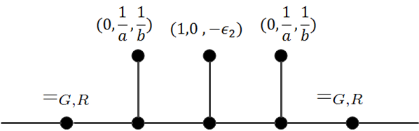
Figure 3: A binary gadget.

Next we use the gadget depicted in Figure 3 to construct another binary function over domain $\{G,R\}$, whose signature is calculated with the techniques of Section 2.4

$$\begin{bmatrix}\epsilon_{1}&1&0\\ \epsilon_{2}&0&1\end{bmatrix}\begin{bmatrix}g+\epsilon_{2}b&-a&0\\ -a&\epsilon_{1}a&0\\ 0&0&0\end{bmatrix}\begin{bmatrix}\epsilon_{1}&\epsilon_{2}\\ 1&0\\ 0&1\end{bmatrix}=\begin{bmatrix}-g-\epsilon_{1}a-\epsilon_{2}b&\epsilon_{1}\epsilon_{2}(g+\epsilon_{1}a+\epsilon_{2}b)\\ \epsilon_{1}\epsilon_{2}(g+\epsilon_{1}a+\epsilon_{2}b)&-g-\epsilon_{2}b\end{bmatrix}.$$

If $g+\epsilon_{1}a+\epsilon_{2}b\neq 0$, this symmetric binary signature can not be of the form $[*,0,*]$ or $[0,*,0]$, and it is not degenerate as its determinant is nonzero. Therefore the problem is #P-hard.

If $g+\epsilon_{1}a+\epsilon_{2}b=0$, we show that this is indeed a tractable case in Theorem 3.1. It is of the second form in Theorem 3.1 where $\mbox{\boldmath$\alpha$}=(0,0,0)^{\tt T},\mbox{\boldmath$\beta_{1}$}=\sqrt[3]{a}(\epsilon_{1},1,0)^{\tt T}$ and $\mbox{\boldmath$\beta_{2}$}=\sqrt[3]{b}(\epsilon_{2},0,1)^{\tt T}$.

If statement (2) $f_{1}=0$ holds for all $(\alpha,\beta,\gamma)$, we have $x=y=0$ or $z=w=0$. If $x=y=0$, the ternary function (16) is as follows

			$g$
		$0$		$w$
	$0$		$0$		$z$
$a$		$0$		$0$		$b$

Then $G$ is separated from $B$-$R$, and by Lemma 5.6, we are done. The case $z=w=0$ is similar.

If statement (3) $f_{1}^{2}=f_{0}f_{2}$ holds for all $(\alpha,\beta,\gamma)$, we have

$$(\alpha x+\beta a)^{2}(\alpha z+\gamma b)^{2}+(\alpha x+\beta a)^{2}(\alpha w+\gamma z)^{2}+(\alpha y+\beta x)^{2}(\alpha z+\gamma b)^{2}=0.$$ (17)

Let $\alpha=a$ and $\beta=-x$, we have $(ay-x^{2})^{2}(az+\gamma b)^{2}=0$ holds for all $\gamma$. Since $b\neq 0$, we can choose $\gamma$ such that $az+\gamma b\neq 0$ and conclude that $ay-x^{2}=0$. Similarly, let $\alpha=b$ and $\gamma=-z$, we can get $bw-z^{2}=0$. Then let $\beta=\gamma=1$ and $\alpha=0$ in (17), we have

$$a^{2}b^{2}+a^{2}z^{2}+b^{2}x^{2}=0.$$

Denote by $p=\frac{x}{a}$ and $q=\frac{z}{b}$, we have $p^{2}+q^{2}+1=0$ and the ternary signature in (16) has the following form

			$g$
		$ap^{2}$		$bq^{2}$
	$ap$		$0$		$bq$
$a$		$0$		$0$		$b$

If $p=0$ or $q=0$, then the function is separable and we are done by Lemma 5.6. In the following, we assume that $pq\neq 0$.

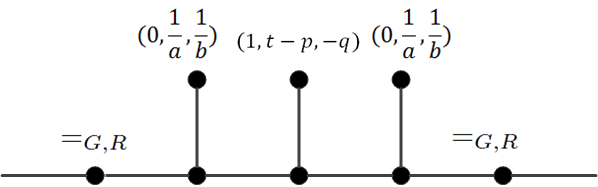
Figure 4: A binary gadget.

Then we use the gadget in Figure 4 to construct another binary function over domain $\{G,R\}$, whose signature is

$$\begin{bmatrix}p&1&0\\ q&0&1\end{bmatrix}\begin{bmatrix}g-bq^{3}-ap^{3}+ap^{2}t&apt&0\\ apt&at&0\\ 0&0&0\end{bmatrix}\begin{bmatrix}p&q\\ 1&0\\ 0&1\end{bmatrix}=\begin{bmatrix}p^{2}\delta+at(p^{2}+1)^{2}&pq\delta+apqt(p^{2}+1)\\ pq\delta+apqt(p^{2}+1)&q^{2}\delta+ap^{2}q^{2}t\end{bmatrix},$$

where $\delta=g-ap^{3}-bq^{3}$. We denote this symmetric binary function as $[g_{0},g_{1},g_{2}]$.

If $\delta=0$, one can verify that this is indeed a tractable case of Theorem 3.1. This is of the third form of Theorem 3.1, where $\mbox{\boldmath$\beta$}=(1,-p,-q)^{\tt T},\mbox{\boldmath$\gamma$}=(0,0,0)^{\tt T}$, and $\mathbf{F}_{\beta}$ is the given function $\mathbf{F}$.

Now we assume that $\delta\neq 0$. If there exists some $t$ such that this binary function is not of the form $[*,0,*]$, $[0,*,0]$, or degenerate, then the problem is #P-hard and we are done. Otherwise, by the same argument as above, at least one of the three statements (i) $g_{0}=g_{2}=0$, (ii) $g_{1}=0$, or (iii) $g_{1}^{2}=g_{0}g_{2}$ holds for all $t$. Choose $t=0$, we have all three $g_{0},g_{1},g_{2}\neq 0$. Therefore, the only possibility is that $g_{1}^{2}=g_{0}g_{2}$ holds for all $t$. However, this is also impossible which can be seen by choosing $t=\frac{1}{a}$. One can calculate the determinant $\det\begin{bmatrix}g_{0}&g_{1}\\ g_{1}&g_{2}\end{bmatrix}=\delta q^{2}\not=0$. This completes the proof for the case $\mathbf{F}^{*{}=\{G,R\}}=H[a,0,0,b]^{\tt T}$.

Case 2: $\mathbf{F}^{*\rightarrow\{G,R\}}=Z[a,0,0,b]^{\tt T},~{}~{}~{}ab\not=0$.

The problem Holant${}^{*}(\{\mathbf{F},=_{G,R}\})$ can be written as Holant${}^{*}(=_{2}|\{\mathbf{F},=_{G,R}\})$, where $*$ means that both sides can use all unary functions. After a holographic transformation under the matrix $\tilde{Z}=\begin{bmatrix}1&\mathbf{0}\\ \mathbf{0}&Z\end{bmatrix}$, we can get an equivalent problem Holant${}^{*}(\neq_{B;G,R}|\{\tilde{Z}^{-1}\mathbf{F},\neq_{G,R}\})$, where the two binary functions are, respectively,

$$(\neq_{B;G,R})=\tilde{Z}^{\tt T}(=_{2})\tilde{Z}=\begin{bmatrix}1&0&0\\ 0&0&1\\ 0&1&0\end{bmatrix},~{}~{}~{}\mbox{and}~{}~{}~{}(\neq_{G,R})=\tilde{Z}^{-1}(=_{G,R})(\tilde{Z}^{-1})^{\tt T}=\begin{bmatrix}0&0&0\\ 0&0&1\\ 0&1&0\end{bmatrix}.$$ (18)

We use $\mathbf{\tilde{F}}$ to denote the ternary function $\tilde{Z}^{-1}\mathbf{F}$ after the transformation. Then we have $\mathbf{\tilde{F}}^{*\rightarrow\{G,R\}}=[a,0,0,b]$. By connecting $\neq_{B;G,R}$ to both sides of $\neq_{G,R}$, we can get the function $\neq_{G,R}$ on the LHS. For a bipartite holant problem Holant${}^{*}([f_{0},f_{1},f_{2}]|[a,0,0,b])$ over domain size 2, the problem is #P-hard unless the binary function $[f_{0},f_{1},f_{2}]$ is of the form $[*,0,*]$, $[0,*,0]$, or degenerate [15]. Therefore, we will try to construct binary functions in the LHS of Holant${}^{*}(\{\neq_{B;G,R},\neq_{G,R}\}|\{\mathbf{\tilde{F}},\neq_{G,R}\})$ over domain $\{G,R\}$.

Our ternary function $\mathbf{\tilde{F}}$ is as follows

			$\tilde{F}_{BBB}$
		$\tilde{F}_{BBG}$		$\tilde{F}_{BBR}$
	$\tilde{F}_{BGG}$		$\tilde{F}_{BGR}$		$\tilde{F}_{BRR}$
$a$		$0$		$0$		$b$

If $\tilde{F}_{BGR}\neq 0$, we can realized a binary function $[\tilde{F}_{BRR},,\tilde{F}_{BGR},\tilde{F}_{BGG}+at]$ over domain $\{G,R\}$ by connecting this ternary function to a unary function $(1,t,0)$ and putting $\neq_{G,R}$ on the other two dangling edges. Since $a\neq 0$ and we can choose any $t$, we can make the third entry of $[\tilde{F}_{BRR},,\tilde{F}_{BGR},\tilde{F}_{BGG}+at]$ arbitrary and the function is not in all three tractable binary forms. Therefore the problem is #P-hard. Now we can assume that $\tilde{F}_{BGR}=0$. To simplify notations, we use variables to denote the function entries as follows

			$g$
		$y$		$w$
	$x$		$0$		$z$
$a$		$0$		$0$		$b$

Then we use the gadget depicted in Figure 5 to construct another binary function in the LHS.

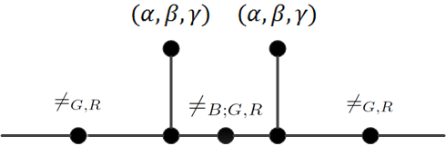
Figure 5: A binary gadget.

The signature of this binary function is

$$[f_{0},f_{1},f_{2}]=[(\alpha w+\gamma z)^{2},(\alpha y+\beta x)(\alpha w+\gamma z)+(\alpha x+\beta a)(\alpha z+\gamma b),(\alpha y+\beta x)^{2}].$$

If there exists some $(\alpha,\beta,\gamma)$ such that this $[f_{0},f_{1},f_{2}]$ is not of the form $[*,0,*]$, $[0,*,0]$, or degenerate, then the problem is #P-hard and we are done. Otherwise, for all $(\alpha,\beta,\gamma)$, we have (1) $f_{0}=f_{2}=0$, (2) $f_{1}=0$, or (3) $f_{1}^{2}=f_{0}f_{2}$. Since all the conditions are polynomials of $(\alpha,\beta,\gamma)$, we can conclude that at least one of the three conditions (1), (2), or (3) holds for all $(\alpha,\beta,\gamma)$.

If condition (1) $f_{0}=f_{2}=0$ holds for all $(\alpha,\beta,\gamma)$, we have $x=y=z=w=0$ and the problem is separable and therefore tractable. And it can be easily verified that this is the second form of Theorem 3.1, where $\mbox{\boldmath$\alpha$}=\sqrt[3]{g}(1,0,0)^{\tt T}$, $\mbox{\boldmath$\beta_{1}$}=\frac{\sqrt[3]{a}}{\sqrt{2}}(0,1,i)^{\tt T}$ and $\mbox{\boldmath$\beta_{2}$}=\frac{\sqrt[3]{b}}{\sqrt{2}}(0,1,-i)^{\tt T}$.

If condition (2) $f_{1}=0$ holds for all $(\alpha,\beta,\gamma)$, we have that

$$xz+yw=xb+yz=az+xw=ab+xz=0.$$

Since $xz=-ab\neq 0$, we can conclude from above that

$$\frac{x}{a}=\frac{y}{x}=p,~{}~{}~{}\frac{z}{b}=\frac{w}{z}=q,~{}~{}~{}\mbox{and}~{}~{}~{}pq=-1.$$

The ternary signature has the form

			$g$
		$ap^{2}$		$bq^{2}$
	$ap$		$0$		$bq$
$a$		$0$		$0$		$b$

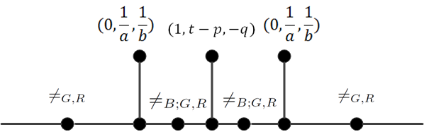
Figure 6: A binary gadget.

Then we use the gadget in Figure 6 to construct another binary function over domain $\{G,R\}$, whose signature is

$$\begin{bmatrix}q&0&1\\ p&1&0\end{bmatrix}\begin{bmatrix}g-bq^{3}-ap^{3}+ap^{2}t&0&apt\\ 0&0&0\\ apt&0&at\end{bmatrix}\begin{bmatrix}q&p\\ 0&1\\ 1&0\end{bmatrix}=\begin{bmatrix}q^{2}\delta+at(pq+1)^{2}&pq\delta+ap^{2}t(pq+1)\\ pq\delta+ap^{2}t(pq+1)&p^{2}\delta+ap^{4}t\end{bmatrix},$$

where $\delta=g-ap^{3}-bq^{3}$. We denote this symmetric binary function as $[g_{0},g_{1},g_{2}]$.

If $\delta=0$, i.e., $g=ap^{3}+bq^{3}$, we show that this is indeed a tractable case of Theorem 3.1 as follows. The ternary function $\mathbf{\tilde{F}}$ can be written as

$$\mathbf{\tilde{F}}=a\begin{bmatrix}p\\ 1\\ 0\end{bmatrix}^{\otimes 3}+b\begin{bmatrix}q\\ 0\\ 1\end{bmatrix}^{\otimes 3}.$$

And

$$\mathbf{F}=\tilde{Z}\mathbf{\tilde{F}}=a\begin{bmatrix}p\\ \frac{1}{\sqrt{2}}\\ \frac{i}{\sqrt{2}}\end{bmatrix}^{\otimes 3}+b\begin{bmatrix}q\\ \frac{1}{\sqrt{2}}\\ -\frac{i}{\sqrt{2}}\end{bmatrix}^{\otimes 3}.$$

This is of the first form of tractable cases in Theorem 3.1, where $\mbox{\boldmath$\alpha$}=\sqrt[3]{a}(p,\frac{1}{\sqrt{2}},\frac{i}{\sqrt{2}})^{\tt T}$, $\mbox{\boldmath$\beta$}=\sqrt[3]{b}(q,\frac{1}{\sqrt{2}},-\frac{i}{\sqrt{2}})^{\tt T}$ and $\mbox{\boldmath$\gamma$}=(0,0,0)^{\tt T}$. We note that the condition $\langle\mbox{\boldmath$\alpha$},\mbox{\boldmath$\beta$}\rangle=0$ is guaranteed by $pq=-1$.

Now we assume that $\delta\neq 0$. If there exists some $t$ such that the binary function $[g_{0},g_{1},g_{2}]$ is not of the form $[*,0,*]$, $[0,*,0]$, or degenerate, then the problem is #P-hard and we are done. Otherwise, by the same argument as above, at least one of the three statements holds for all $t$: (i) $g_{0}=g_{2}=0$, (ii) $g_{1}=0$, or (iii) $g_{1}^{2}=g_{0}g_{2}$. Choose $t=0$, we have $g_{0}g_{1}g_{2}\neq 0$. Therefore, the only possibility is that $g_{1}^{2}=g_{0}g_{2}$ holds for all $t$. However, this is also a contradiction which can be seen by choosing $t=\frac{1}{a}$. One can calculate the determinant $\det\begin{bmatrix}g_{0}&g_{1}\\ g_{1}&g_{2}\end{bmatrix}=\delta p^{2}\not=0$.

If condition (3) $f_{1}^{2}=f_{0}f_{2}$ holds for all $(\alpha,\beta,\gamma)$, we have

$$0=f_{1}^{2}-f_{0}f_{2}=2(\alpha y+\beta x)(\alpha w+\gamma z)(\alpha x+\beta a)(\alpha z+\gamma b)+(\alpha x+\beta a)^{2}(\alpha z+\gamma b)^{2}.$$ (19)

Let $\alpha=x$ and $\beta=-y$, we have $(x^{2}-ay)^{2}(xz+\gamma b)^{2}=0$ holds for all $\gamma$. Since $b\neq 0$, we conclude that $ay-x^{2}=0$. Similarly, let $\alpha=z$ and $\gamma=-w$, we can get $bw-z^{2}=0$. Then let $\beta=\gamma=1$ and $\alpha=0$ in (19), we have

$$ab+2xz=0.$$

Denote by $p=\frac{x}{a}$ and $q=\frac{z}{b}$, we have $pq=-\frac{1}{2}$ and the ternary signature has the form

			$g$
		$ap^{2}$		$bq^{2}$
	$ap$		$0$		$bq$
$a$		$0$		$0$		$b$

Figure 7: A binary gadget.

Then we use the gadget in Figure 7 to construct another binary function over domain $\{G,R\}$, whose signature is

$$\begin{bmatrix}q&0&1\\ p&1&0\end{bmatrix}\begin{bmatrix}g-bq^{3}-ap^{3}+ap^{2}t&0&apt\\ 0&0&0\\ apt&0&at\end{bmatrix}\begin{bmatrix}q&p\\ 0&1\\ 1&0\end{bmatrix}=\begin{bmatrix}q^{2}\delta+at(pq+1)^{2}&pq\delta+ap^{2}t(pq+1)\\ pq\delta+ap^{2}t(pq+1)&p^{2}\delta+ap^{4}t\end{bmatrix},$$

where $\delta=g-ap^{3}-bq^{3}$. We denote this symmetric binary function as $[g_{0},g_{1},g_{2}]$. (This is the same construction as in Figure 6, but $p$ and $q$ have a different meaning.)

If $\delta=0$, we show that this is indeed a tractable case of Theorem 3.1 as follows. The ternary function $\mathbf{\tilde{F}}$ can be written as

$$\mathbf{\tilde{F}}=a\begin{bmatrix}p\\ 1\\ 0\end{bmatrix}^{\otimes 3}+b\begin{bmatrix}q\\ 0\\ 1\end{bmatrix}^{\otimes 3}.$$

And

$$\mathbf{F}=\tilde{Z}\mathbf{\tilde{F}}=a\begin{bmatrix}p\\ \frac{1}{\sqrt{2}}\\ \frac{i}{\sqrt{2}}\end{bmatrix}^{\otimes 3}+b\begin{bmatrix}q\\ \frac{1}{\sqrt{2}}\\ -\frac{i}{\sqrt{2}}\end{bmatrix}^{\otimes 3}.$$

This is of the third form of tractable case in Theorem 3.1, where $\mathbf{F}_{\beta}$ is the given function $\mathbf{F}$ and $\mbox{\boldmath$\beta$}=(-\sqrt{2},p+q,-pi+qi)^{\tt T},\mbox{\boldmath$\gamma$}=(0,0,0)^{\tt T}$. We note that $pq=-\frac{1}{2}$ implies that $\langle\mbox{\boldmath$\beta$},\mbox{\boldmath$\beta$}\rangle=0$.

Now we assume that $\delta\neq 0$. If there exists some $t$ such that this binary function is not of the form $[*,0,*]$, $[0,*,0]$, or degenerate, then the problem is #P-hard and we are done. Otherwise, by the same argument as above, at least one of the three (i) $g_{0}=g_{2}=0$, (ii) $g_{1}=0$, or (iii) $g_{1}^{2}=g_{0}g_{2}$ holds for all $t$. Choose $t=0$, we have $g_{0}g_{1}g_{2}\neq 0$. Therefore, the only possibility is that $g_{1}^{2}=g_{0}g_{2}$ holds for all $t$. However, this is also a contradiction which can be seen by choosing $t=\frac{1}{a}$. One can calculate the determinant $\det\begin{bmatrix}g_{0}&g_{1}\\ g_{1}&g_{2}\end{bmatrix}=\delta p^{2}\not=0$. This completes the proof for the case $\mathbf{F}^{*\rightarrow\{G,R\}}=Z[a,0,0,b]^{\tt T}$.

Case 3: $\mathbf{F}^{*\rightarrow\{G,R\}}=Z[a,b,0,0]^{\tt T},~{}~{}~{}b\not=0$.

Here we only prove for the case $Z=\frac{1}{\sqrt{2}}\begin{bmatrix}1&1\\ i&-i\end{bmatrix}$. The other case is symmetric. The Holant problem can be written as Holant${}^{*}(=_{2}|\{\mathbf{F},=_{G,R}\})$, where $*$ means that both sides can use unary functions. After a holographic transformation under the matrix $\tilde{Z}=\begin{bmatrix}1&\mathbf{0}\\ \mathbf{0}&Z\end{bmatrix}$, we can get an equivalent problem Holant${}^{*}(\neq_{B;G,R}|\{\tilde{Z}^{-1}\mathbf{F},\neq_{G,R}\})$, where the two binary functions $\neq_{B;G,R}$ and $\neq_{G,R}$ are given in (18). We use $\mathbf{\tilde{F}}$ to denote this ternary function after the transformation $\tilde{Z}^{-1}\mathbf{F}$. Then we have $\mathbf{\tilde{F}}^{*\rightarrow\{G,R\}}=[a,b,0,0]$. And after a scaling, we assume that $\mathbf{\tilde{F}}^{*\rightarrow\{G,R\}}=[a,1,0,0]$. By connecting $\neq_{B;G,R}$ to both sides of $\neq_{G,R}$, we can get a $\neq_{G,R}$ on the LHS. For a bipartite holant problem Holant${}^{*}([f_{0},f_{1},f_{2}]|[a,1,0,0])$ over domain size 2, the problem is #P-hard unless the binary function $[f_{0},f_{1},f_{2}]$ is of the form $[0,*,*]$ or degenerate. This can be seen as follows: Clearly for such $[f_{0},f_{1},f_{2}]$ it is tractable, as $[0,*,*]$ requires the number of edges assigned 0 to be at most the number assigned 1, while $[a,1,0,0]$ requires the number of edges assigned 0 to be strictly more than the number assigned 1. Suppose $[f_{0},f_{1},f_{2}]$ is nondegenerate and not of this form, we may normalize it to $[1,b,c]$ where $c\not=b^{2}$. Consider the holographic reduction defined by $M=\begin{bmatrix}1&b\\ 0&\sqrt{c-b^{2}}\end{bmatrix}$. The matrix form for $[1,0,1]M^{\otimes 2}$ is $M^{\tt T}I_{2}M=\begin{bmatrix}1&b\\ b&c\end{bmatrix}$, namely $[1,b,c]$, while $M^{\otimes 3}[a,1,0,0]$ is

$$\begin{bmatrix}1&b\\ 0&\sqrt{c-b^{2}}\end{bmatrix}^{\otimes 3}\left[a\begin{bmatrix}1\\ 0\end{bmatrix}^{\otimes 3}+\begin{bmatrix}1\\ 0\end{bmatrix}\otimes\begin{bmatrix}1\\ 0\end{bmatrix}\otimes\begin{bmatrix}0\\ 1\end{bmatrix}+\begin{bmatrix}1\\ 0\end{bmatrix}\otimes\begin{bmatrix}0\\ 1\end{bmatrix}\otimes\begin{bmatrix}1\\ 0\end{bmatrix}+\begin{bmatrix}0\\ 1\end{bmatrix}\otimes\begin{bmatrix}1\\ 0\end{bmatrix}\otimes\begin{bmatrix}1\\ 0\end{bmatrix}\right],$$

which is $[a+3b,\sqrt{c-b^{2}},0,0]$. By Theorem 2.5, Holant${}^{*}([a+3b,\sqrt{c-b^{2}},0,0])$ is #P-hard. Therefore, to show #P-hardness, we will construct binary functions in the LHS of Holant${}^{*}(\{\neq_{B;G,R},\neq_{G,R}\}|\mathbf{\tilde{F}})$ over domain $\{G,R\}$.

Now we have the ternary function $\mathbf{\tilde{F}}$ as follows

			$\tilde{F}_{BBB}$
		$\tilde{F}_{BBG}$		$\tilde{F}_{BBR}$
	$\tilde{F}_{BGG}$		$\tilde{F}_{BGR}$		$\tilde{F}_{BRR}$
$a$		$1$		$0$		$0$

If $\tilde{F}_{BRR}\neq 0$, we can realized a binary function $[\tilde{F}_{BRR},\tilde{F}_{BGR}+t,\tilde{F}_{BGG}+at]$ in LHS over domain $\{G,R\}$ by connecting this ternary function to a unary function $(1,t,0)$ and putting $\neq_{G,R}$ on the other two dangling edges. It can be easily seen that we can choose some $t$ such that $[\tilde{F}_{BRR},\tilde{F}_{BGR}+t,\tilde{F}_{BGG}+at]$ is not degenerate. And it is not of the form $[0,*,*]$ since $\tilde{F}_{BRR}\neq 0$. Therefore the problem is #P-hard. Now we can assume that $\tilde{F}_{BRR}=0$. To simplify notations, we use variables to denote the function entries of $\mathbf{\tilde{F}}$ as follows

$$g$$

(20)

Then we use the gadget in Figure 8 to construct another binary function.

Figure 8: A binary gadget.

The signature of this binary function is

$$[f_{0},f_{1},f_{2}]=[(\alpha w+\beta y)^{2},(\alpha w+\beta y)(\alpha z+\beta x+\gamma y)+(\alpha y+\beta)^{2},(\alpha z+\beta x+\gamma y)^{2}+2(\alpha y+\beta)(\alpha x+\beta a+\gamma)].$$

If there exists some $(\alpha,\beta,\gamma)$ such that this $[f_{0},f_{1},f_{2}]$ is not of the form $[0,*,*]$ or degenerate, then the problem is #P-hard and we are done. Otherwise, for all $(\alpha,\beta,\gamma)$, we have the equalities (1) $f_{0}=0$ or (2) $f_{1}^{2}=f_{0}f_{2}$. Since these are polynomials of $(\alpha,\beta,\gamma)$, at least one of (1) $f_{0}=0$ or (2) $f_{1}^{2}=f_{0}f_{2}$ holds for all $(\alpha,\beta,\gamma)$.

If equality (1) $f_{0}=0$ holds for all $(\alpha,\beta,\gamma)$, we have $y=w=0$. We will verify that the problem is tractable, and it is of the third form of Theorem 3.1. We use $\mathbf{\tilde{F}}_{\beta}$ to denote the following ternary function

			$g$
		$z$		$0$
	$x$		$0$		$0$
$a$		$0$		$0$		$0$

Let $\tilde{\beta}=(0,1,0)^{\tt T}$ and $\tilde{\gamma}=(0,0,1)^{\tt T}$. Compared to (20) we have

$$\mathbf{\tilde{F}}=\mathbf{\tilde{F}_{\beta}}+\mathbf{\tilde{\beta}}^{\otimes 2}\otimes\tilde{\gamma}+\tilde{\beta}\otimes\tilde{\gamma}\otimes\tilde{\beta}+\tilde{\gamma}\otimes\mathbf{\tilde{\beta}}^{\otimes 2}.$$

Therefore applying the transformation $\tilde{Z}$, we have

$$\mathbf{F}=\tilde{Z}\mathbf{\tilde{F}}=\tilde{Z}\mathbf{\tilde{F}_{\beta}}+{(\tilde{Z}\tilde{\beta})}^{\otimes 2}\otimes(\tilde{Z}\tilde{\gamma})+(\tilde{Z}\tilde{\beta})\otimes(\tilde{Z}\tilde{\gamma})\otimes(\tilde{Z}\tilde{\beta})+(\tilde{Z}\tilde{\gamma})\otimes{(\tilde{Z}\tilde{\beta})}^{\otimes 2}.$$

We verify that this is in the third form of Theorem 3.1, with $\mathbf{F}_{\beta}=\tilde{Z}\mathbf{\tilde{F}_{\beta}}$, $\mbox{\boldmath$\beta$}=\tilde{Z}\tilde{\beta}$ and $\mbox{\boldmath$\gamma$}=\tilde{Z}\tilde{\gamma}$. First it is easy to verify that $\langle\mbox{\boldmath$\beta$},\mbox{\boldmath$\beta$}\rangle=0$. Second $\langle(0,0,1),\mathbf{\tilde{F}_{\beta}}\rangle=\mathbf{0}$, and $\tilde{\beta}^{\tt T}\tilde{Z}^{T}\tilde{Z}=(0,0,1)$, hence

$$\langle\mbox{\boldmath$\beta$},\mathbf{{F}_{\beta}}\rangle=\mathbf{0}.$$

If equality (2) $f_{1}^{2}=f_{0}f_{2}$ holds for all $(\alpha,\beta,\gamma)$, we have

$$0=f_{0}f_{2}-f_{1}^{2}=(\alpha y+\beta)(2(\alpha w+\beta y)^{2}(\alpha x+\beta a+\gamma)-2(\alpha w+\beta y)(\alpha z+\beta x+\gamma y)(\alpha y+\beta)-(\alpha y+\beta)^{3}).$$

As a product of two polynomials in $(\alpha,\beta,\gamma)$, to be identically zero, one of them must be identically zero. Since $\alpha y+\beta$ is not identically zero, we have

$$2(\alpha w+\beta y)^{2}(\alpha x+\beta a+\gamma)-2(\alpha w+\beta y)(\alpha z+\beta x+\gamma y)(\alpha y+\beta)-(\alpha y+\beta)^{3}=0,$$ (21)

for all $(\alpha,\beta,\gamma)$.

Let $\alpha=y$ and $\beta=-w$, we have $w=y^{2}$. Substituting $w=y^{2}$ in (21), we have

$$2y^{2}(\alpha x+\beta a+\gamma)-2y(\alpha z+\beta x+\gamma y)-(\alpha y+\beta)=0,$$

for all $(\alpha,\beta,\gamma)$. And we conclude that $y(2xy-2z-1)=0$ and $2ay^{2}-2xy-1=0$. The second equation implies that $y\not=0$. So we have $2xy-2z-1=0$.

Then the ternary signature has the form

$$g$$

(22)

If $g=ay^{3}-\frac{3}{2}y$, we show that this problem is indeed tractable. We show that this $\mathbf{F}$ is of the third form in Theorem 3.1, where $\mathbf{F}_{\beta}$ is the given function $\mathbf{F}$, and

$$\mbox{\boldmath$\beta$}=(1,-\frac{y}{\sqrt{2}}+\frac{1}{2\sqrt{2}y},\frac{yi}{\sqrt{2}}+\frac{i}{2\sqrt{2}y})^{\tt T},~{}~{}~{}~{}\mbox{\boldmath$\gamma$}=(0,0,0)^{\tt T}.$$

First it is easy to verify that $\langle\mbox{\boldmath$\beta$},\mbox{\boldmath$\beta$}\rangle=0$. We also need to verify $\langle\mbox{\boldmath$\beta$},\mathbf{F}\rangle=\mathbf{0}$, or $\langle\mbox{\boldmath$\beta$},\tilde{Z}\mathbf{\tilde{F}}\rangle=\mathbf{0}$, which is equivalent to $\langle\tilde{Z}^{\tt T}\mbox{\boldmath$\beta$},\mathbf{\tilde{F}}\rangle=\mathbf{0}$. This $\tilde{Z}^{\tt T}\mbox{\boldmath$\beta$}$ is $(1,-y,\frac{1}{2y})^{\tt T}$, and it is easy to see that indeed this unary function annihilates $\mathbf{\tilde{F}}$ in (22), using the “calculus” from Section 2.4.

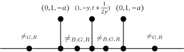
Figure 9: A binary gadget.

Now we assume that $g\neq ay^{3}-\frac{3}{2}y$. We denote by $\delta=g-ay^{3}+\frac{3}{2}y$. Then we use the gadget in Figure 9 to construct another binary function over domain $\{G,R\}$, whose signature is

$$\begin{bmatrix}y&1&0\\ -\frac{1}{2y}&0&1\end{bmatrix}\begin{bmatrix}\delta+y^{2}t&0&yt\\ 0&0&0\\ yt&0&t\end{bmatrix}\begin{bmatrix}y&-\frac{1}{2y}\\ 1&0\\ 0&1\end{bmatrix}=\begin{bmatrix}y^{2}\delta+y^{4}t&-\frac{\delta}{2}+\frac{y^{2}t}{2}\\ -\frac{\delta}{2}+\frac{y^{2}t}{2}&\frac{\delta}{4y^{2}}+\frac{t}{4}\end{bmatrix}.$$

We denote this symmetric binary function as $[g_{0},g_{1},g_{2}]$. If there exists some $t$ such that this binary function is not of the form $[0,*,*]$, or degenerate, then the problem is #P-hard and we are done. Otherwise, by the same argument as above, at least one of the two equations (i) $g_{0}=0$ or (ii) $g_{1}^{2}=g_{0}g_{2}$ holds for all $t$. Choose $t=0$, we have $g_{0}=y^{2}\delta\neq 0$. Choose $t=\frac{\delta}{y^{2}}$, we can verify that the signature is not degenerate. This completes the proof for the case $\mathbf{F}^{*\rightarrow\{G,R\}}=Z[a,b,0,0]^{\tt T}$.

We have completed the proof of Theorem 5.7 when $\mathbf{F}^{*\rightarrow\{G,R\}}$ is non-degenerate.

5.4 $\mathbf{F}^{*\rightarrow\{G,R\}}$ is $[1,0,0,0]$ After an Orthogonal Transformation

We have proved our dichotomy theorem Theorem 3.1 when $\mathbf{F}^{*\rightarrow\{G,R\}}$ is non-degenerate. In the rest of this paper we deal with the case when $\mathbf{F}^{*\rightarrow\{G,R\}}$ is degenerate. We first suppose it has rank 1, and therefore has the form $(a,b)^{\otimes 3}$. In this subsection we assume $(a,b)$ is non-isotropic.

Thus, possibly after a reversal, which is an orthogonal transformation, $\mathbf{F}^{*\rightarrow\{G,R\}}$ is degenerate of the form $c[1,\lambda,\lambda^{2},\lambda^{3}]^{\tt T}$, where $c\not=0$ and $\lambda\not\in\{i,-i\}$. As $(1,\lambda)$ is not isotropic, we can perform an orthogonal transformation, after which, and ignoring a non-zero scalar multiple, we may assume the bottom line $\mathbf{F}^{*\rightarrow\{G,R\}}$ is $[1,0,0,0]^{\tt T}$.

Suppose $\mathbf{F}=[u;t,r;s,p,q;1,0,0,0]$, namely

$$u$$

(23)

Our general method will be to construct some gadgets which can realize certain functions, and under some conditions we can use them to show that Holant${}^{*}(\mathbf{F})$ is #P-hard. We first construct the following function $\mathbf{H}(x_{1},x_{2},x_{3},x_{4})=(\sum_{y\in\{B,G,R\}}\mathbf{F}(x_{1},x_{2},y)\mathbf{F}(y,x_{3},x_{4}))^{*\rightarrow\{G,R\}}$, which can be realized by connecting two copies of $\mathbf{F}$ by one edge, and then connecting $=_{B,G}$ on all four external edges. Denote by $\mathcal{T}$ the set of functions of arity at most 2, and $\langle\mathcal{T}\rangle$ the tensor product closure of $\mathcal{T}$.

Lemma 5.8.

If $p\neq 0$ or $q\neq 0$, then $\mathbf{H}\not\in\langle\mathcal{T}\rangle$.

Proof.

By the definition of $\mathbf{H}$, we have $\mathbf{H}(x_{1},x_{2},x_{3},x_{4})=\mathbf{H}(x_{2},x_{1},x_{3},x_{4})=\mathbf{H}(x_{1},x_{2},x_{4},x_{3})$, because $\mathbf{F}$ is a symmetric function. We prove the lemma by a contradiction. Suppose $\mathbf{H}\in\langle\mathcal{T}\rangle$. Then, either $\mathbf{H}(x_{1},x_{2},x_{3},x_{4})=\mathbf{P}(x_{1},x_{2})\mathbf{Q}(x_{3},x_{4})$, or $\mathbf{H}(x_{1},x_{2},x_{3},x_{4})=\mathbf{P}(x_{1},x_{3})\mathbf{Q}(x_{2},x_{4})$ for some binary functions $\mathbf{P}$ and $\mathbf{Q}$.

The matrix form $\mathbf{H}_{x_{1}x_{2},~{}x_{3}x_{4}}$ (whose rows are indexed by $x_{1}x_{2}$ and columns are indexed by $x_{3}x_{4}$, and are in the order $GG,GR,RG,RR$) of the function $\mathbf{H}$ is

$$\left[\begin{array}[]{cccc}s^{2}+1&sp&sp&sq\\ sp&p^{2}&p^{2}&pq\\ sp&p^{2}&p^{2}&pq\\ sq&pq&pq&q^{2}\end{array}\right].$$

If $\mathbf{H}(x_{1},x_{2},x_{3},x_{4})=\mathbf{P}(x_{1},x_{2})\mathbf{Q}(x_{3},x_{4})$ for some binary functions $\mathbf{P}$ and $\mathbf{Q}$, then $\mathbf{H}_{x_{1}x_{2},~{}x_{3}x_{4}}=\mathbf{P}_{4\times 1}(\mathbf{Q}_{4\times 1})^{\tt T}$ has rank at most 1, where we use the vector form $\mathbf{P}_{4\times 1}$ and $\mathbf{Q}_{4\times 1}$ for the functions $\mathbf{P}$ and $\mathbf{Q}$. This implies that $p=q=0$, by taking some $2\times 2$ determinantal minors. A contradiction.

The matrix form $\mathbf{H}_{x_{1}x_{3},~{}x_{2}x_{4}}$ (also in index order $GG,GR,RG,RR$) of the function $\mathbf{H}$ is

$$\left[\begin{array}[]{cccc}s^{2}+1&sp&sp&p^{2}\\ sp&sq&p^{2}&pq\\ sp&p^{2}&sq&pq\\ p^{2}&pq&pq&q^{2}\end{array}\right].$$

If $\mathbf{H}(x_{1},x_{2},x_{3},x_{4})=\mathbf{P}(x_{1},x_{3})\mathbf{Q}(x_{2},x_{4})$ for some binary functions $\mathbf{P}$ and $\mathbf{Q}$, by the same argument, the matrix $\mathbf{H}_{x_{1}x_{3},~{}x_{2}x_{4}}$ has rank at most 1. If $p\neq 0$, then because the submatrix indexed by $(RG,RR)\times(GG,GR)$ is singular, we get $sq=p^{2}$. Similarly if $q\neq 0$, by the submatrix indexed by $(RG,RR)\times(RG,RR)$, we also get $sq=p^{2}$. Hence, $sq=p^{2}$ holds. We also have the determinantal minor indexed by $(GG,GR)\times(GG,GR)$, $\left|\begin{array}[]{cc}s^{2}+1&sp\\ sp&sq\end{array}\right|=p^{2}=0$ and the minor indexed by $(GG,RR)\times(GG,RR)$, $\left|\begin{array}[]{cc}s^{2}+1&p^{2}\\ p^{2}&q^{2}\end{array}\right|=q^{2}=0$. A contradiction. ∎

We have proved that $\mathbf{H}\not\in\langle\mathcal{T}\rangle$ under the condition $p\neq 0$ or $q\neq 0$.

Lemma 5.9.

In Holant${}^{*}(\mathbf{F})$, if $p\neq 0$ or $q\neq 0$, either for each tractable class $\mathcal{P}_{a,b}$ and $\mathcal{P}$, we can construct a symmetric non-degenerate binary function not in it, or the domain is separated and the complexity dichotomy holds.

Proof.

Define binary functions $\mathbf{R}_{x}=\langle(1,x,0),\mathbf{F}\rangle^{*\rightarrow\{G,R\}}$, which are clearly realizable, where $x$ is an arbitrary (algebraic) complex number. In symmetric signature notation on the Boolean domain $\mathbf{R}_{x}=[s+x,p,q]$. If $p\neq 0$ or $q\neq 0$, there is at most one value $x$ such that $\mathbf{R}_{x}$ is degenerate. Assume $p\neq 0$. For any $a\neq 0$, obviously there exists an $x$ such that a non-degenerate $\mathbf{R}_{x}\not\in\mathcal{P}_{a,b}$, since the coefficient of $x$ in the linear equation requirement for $\mathbf{R}_{x}\in\mathcal{P}_{a,b}$ (for both alternative forms in $\mathcal{P}_{a,b}$) is not zero. For $a=0$, then $b\not=0$, and because the middle entry of $\mathbf{R}_{x}$ is $p\neq 0$, there exists an $x$ such that a non-degenerate $\mathbf{R}_{x}\not\in\mathcal{P}_{0,b}$. By the same reasoning, there exists an $x$ such that a non-degenerate $\mathbf{R}_{x}\not\in\mathcal{P}$. This completes the proof of the lemma for the case $p\not=0$.

If $p=0$, we have $q\neq 0$. For each tractable class $\mathcal{P}_{a,b}$ and $\mathcal{P}$, except for $\mathcal{P}_{0,b}$, the function $\mathbf{R}_{x}$ still handles it for all but finitely many values of $x$. The exception is $\mathcal{P}_{0,b}$, which has the normalized form $\mathcal{P}_{0,1}$. We prove this case according to $s\neq 0$ or $s=0$.

The matrix form $\mathbf{H}_{x_{1}x_{2},~{}x_{3}x_{4}}$ (in index order $GG,GR,RG,RR$) of the function $\mathbf{H}$ is

$$\left[\begin{array}[]{cccc}s^{2}+1&sp&sp&sq\\ sp&p^{2}&p^{2}&pq\\ sp&p^{2}&p^{2}&pq\\ sq&pq&pq&q^{2}\end{array}\right]=\left[\begin{array}[]{cccc}s^{2}+1&0&0&sq\\ 0&0&0&0\\ 0&0&0&0\\ sq&0&0&q^{2}\end{array}\right].$$

Since $q\not=0$, the following binary function on $x_{1},x_{3}$ is non-degenerate and realizable

$$\sum_{x_{2},x_{4}\in\{G,R\}}\mathbf{H}(x_{1},x_{2},x_{3},x_{4})=[s^{2}+1,sq,q^{2}].$$

For $s\neq 0$ (and $q\not=0$), it is easy to check that $[s^{2}+1,sq,q^{2}]\not\in\mathcal{P}_{0,1}$.

Now we suppose $s=0$ (and $p=0$), the simpler construction does not work and we use a slightly more complicated construction. Suppose the binary function $\mathbf{P}=\langle(\alpha,\beta,\gamma),\mathbf{F}\rangle=\left[\begin{array}[]{ccc}a&b&c\\ b&e&d\\ c&d&f\end{array}\right]$, where $\alpha,\beta,\gamma$ are to be determined. We construct

$$\mathbf{Q}(x_{1},x_{2},x_{3},x_{4})=\left(\sum_{y_{1},y_{2}\in\{B,G,R\}}\mathbf{F}(x_{1},x_{2},y_{1})\mathbf{P}(y_{1},y_{2})\mathbf{F}(y_{2},x_{3},x_{4})\right)^{*\rightarrow\{G,R\}}.$$

This is realizable by connecting three copies of $\mathbf{F}$ in a chain with the middle copy connected to a unary $(\alpha,\beta,\gamma)$ on one edge, and then connecting $=_{B,G}$ on four external edges. The matrix form $\mathbf{Q}_{x_{1}x_{2},~{}x_{3}x_{4}}$ (in index order $GG,GR,RG,RR$) of the function $\mathbf{Q}$ is

$$\begin{bmatrix}s&1&0\\ p&0&0\\ p&0&0\\ q&0&0\end{bmatrix}\begin{bmatrix}a&b&c\\ b&e&d\\ c&d&f\end{bmatrix}\begin{bmatrix}s&p&p&q\\ 1&0&0&0\\ 0&0&0&0\end{bmatrix}=\begin{bmatrix}as^{2}+2bs+e&asp+bp&asp+bp&asq+bq\\ asp+bp&ap^{2}&ap^{2}&apq\\ asp+bp&ap^{2}&ap^{2}&apq\\ asq+bq&apq&apq&aq^{2}\end{bmatrix}=\begin{bmatrix}e&0&0&bq\\ 0&0&0&0\\ 0&0&0&0\\ bq&0&0&aq^{2}\end{bmatrix}.$$

Let $\mathbf{S}=\sum_{x_{2},x_{4}\in\{G,R\}}\mathbf{Q}(x_{1},x_{2},x_{3},x_{4})=[e,bq,aq^{2}]$, which is realizable. We want to show that there exists $(\alpha,\beta,\gamma)$ such that a non-degenerate $\mathbf{S}\not\in\mathcal{P}_{0,1}$. This means a non-degenerate $\mathbf{S}$ satisfies $bq\neq 0$ and ($e\neq 0$ or $aq^{2}\neq 0$). The violation of these requirements are specified by polynomial equations on $(\alpha,\beta,\gamma)$, therefore we only need to show there exists $(\alpha,\beta,\gamma)$ satisfying each condition separately.

By definition $e=P_{GG}=s\alpha+1\beta+0\gamma=\beta$ is not the zero polynomial (in $\alpha,\beta,\gamma$). Similarly, by the “calculus” from Section 2.4, $a=P_{BB}=u\alpha+t\beta+r\gamma$ and $b=P_{BG}=t\alpha$. $\mathbf{S}$ is non-degenerate iff $b^{2}-ae\neq 0$, since $q\not=0$. If $t\neq 0$, then $b^{2}-ae$, $bq$ and $e$ are all non-zero polynomials in $\alpha,\beta,\gamma$. Hence, if $t\neq 0$, we can get a non-degenerate binary function not in $\mathcal{P}_{0,1}$.

If $t=0$ (and $p=s=0$), for the domain of $\mathbf{F}$, $\{G\}$ is separated from $\{B,R\}$. The validity of Theorem 3.1 for such cases follows from the complexity dichotomy Theorem 2.5. ∎

The two lemmas above solve the case $p\neq 0$ or $q\neq 0$. Now, we consider $p=q=0$, and $\mathbf{F}=[u;t,r;s,0,0;1,0,0,0]$:

			$u$
		$t$		$r$
	$s$		$0$		$0$
$1$		$0$		$0$		$0$

If $r=0$, the domain is separated, and this is handled as before.

Now we suppose $r\neq 0$.

Lemma 5.10.

For $\mathbf{F}$ given in (23) where $p=q=0$ and $r\not=0$, (i.e., $\mathbf{F}$ is given in the table above with $r\not=0$), the problem Holant${{}^{*}}(\mathbf{F})$ is #P-hard, unless $s=t=0$ and the domain is separated (in which case Theorem 3.1 holds).

Proof.

Consider $\langle(0,1,x),\mathbf{F}\rangle=[t+xr;s,0;1,0,0]$, for any complex $x$. This is

		$t+xr$
	$s$		$0$
$1$		$0$		$0$

We can pick an $x$, and use it to realize $=_{B,G}$ by interpolation. Then we can utilize $=_{B,G}$ to reduce a #P-hard problem on the Boolean domain $\{B,G\}$ to Holant${{}^{*}}(\mathbf{F})$.

Over the domain $\{B,G\}$, we try to prove the following: We construct a function not in $\langle\mathcal{T}\rangle$, and for each tractable class $\mathcal{P}_{a,b}$ and $\mathcal{P}$, we construct a binary function not in it. We construct binary functions first.

• $s\neq 0$

  By choosing an $x$, we can realize a non-degenerate binary function $[t+xr,s,1]$ in domain $\{B,G\}$ using $\langle(0,1,x),\mathbf{F}\rangle$ and $=_{B,G}$. The rest of the proof is the same: For each tractable class $\mathcal{P}_{a,b}$ and $\mathcal{P}$, we find a suitable $x$ such that a non-degenerate $[t+xr,s,1]$ does not belong to $\mathcal{P}_{a,b}$ and $\mathcal{P}$.

• $s=0$

  $\diamond$ $t=0$

  The domain is separated.

  $\diamond$ $t\neq 0$

  For any $x$, we can realize a non-degenerate binary function $[u+xr,t,0]$ in domain $\{B,G\}$ using $\langle(1,0,x),\mathbf{F}\rangle$ and $=_{B,G}$. For each tractable class $\mathcal{P}_{a,b}$ and $\mathcal{P}$, there is some $x$ such that $[u+xr,t,0]$ is non-degenerate and not in the class.

Now we construct a suitable ternary function. Obviously, we can realize the ternary function $[u,t,s,1]$ in domain $\{B,G\}$, using $=_{B,G}$. If it is not in $\langle\mathcal{T}\rangle$, we are done.

Suppose we have $[u,t,s,1]\in\langle\mathcal{T}\rangle$. A symmetric ternary signature $[u,t,s,1]$ being decomposable in $\langle\mathcal{T}\rangle$ can only be degenerate, of the form $(s,1)^{\otimes 3}$. That is, $\mathbf{F}=[s^{3};s^{2},r;s,0,0;1,0,0,0]$.

			$s^{3}$
		$s^{2}$		$r$
	$s$		$0$		$0$
$1$		$0$		$0$		$0$

We construct $\langle(1,-s,1),\mathbf{F}\rangle=[r;0,r;0,0,0]$, which is

		$r$
	$0$		$r$
$0$		$0$		$0$

We can use this to realize $=_{B,R}$ by interpolation, using the fact that $r\not=0$. Then on domain $\{B,R\}$, the problem Holant${}^{*}(\mathbf{F^{\prime}})$ is #P-hard for $\mathbf{F^{\prime}}=\mathbf{F}^{*\rightarrow\{B,R\}}=[s^{3},r,0,0]$.

∎

5.5 $\mathbf{F}^{*\rightarrow\{G,R\}}$ Is Degenerate Of Rank 1 And Isotropic

Suppose $\mathbf{F}^{*\rightarrow\{G,R\}}$ is degenerate of rank 1, therefore of the form $(a,b)^{\otimes 3}$, however in this subsection we assume $(a,b)$ is isotropic. The high level proof strategy is similar to that of subsection 5.4, but the execution is considerably more complicated. We only need to prove the case when $\mathbf{F}^{*\rightarrow\{G,R\}}$ is $[1,i,-1,-i]$. The case with $[1,-i,-1,i]$ is the same, and follows formally by taking the conjugation. Let $\mathbf{F}=[u;t,r;s,p,q;1,i,-1,-i]$, namely

$$u$$

(24)

Suppose $\mathbf{T}=\langle(\alpha,\beta,\gamma),\mathbf{F}\rangle=\alpha\mathbf{A}+\beta\mathbf{B}+\gamma\mathbf{C}$, where $\mathbf{A}=\mathbf{F}^{1=B}$, $\mathbf{B}=\mathbf{F}^{1=G}$ and $\mathbf{C}=\mathbf{F}^{1=R}$. Construct

$$\mathbf{H}(x_{1},x_{2},x_{3},x_{4})=\left(\sum_{y_{1},y_{2}\in\{B,G,R\}}\mathbf{F}(x_{1},x_{2},y_{1})\mathbf{T}(y_{1},y_{2})\mathbf{F}(y_{2},x_{3},x_{4})\right)^{*\rightarrow\{G,R\}}.$$

Because $\mathbf{F}$ is symmetric, $\mathbf{H}$ satisfies the condition in Fact 5, and we can use the partial symmetry argument to prove it is not in $\langle\mathcal{T}\rangle$, by showing two decompositions are impossible.

Let $\mathbf{S}=\left[\begin{array}[]{ccc}s&1&i\\ p&i&-1\\ p&i&-1\\ q&-1&-i\end{array}\right]$, indexed by $\{G,R\}^{2}\times\{B,G,R\}$ in lexicographic order. Then the arity 4 function $\mathbf{H}$ has a matrix form $\mathbf{H}_{1}=\mathbf{S}\mathbf{T}\mathbf{S}^{\tt T}$, where the rows are indexed by $(x_{1},x_{2})\in\{G,R\}^{2}$ and the columns are indexed by $(x_{3},x_{4})\in\{G,R\}^{2}$. The other matrix form of $\mathbf{H}$ is $\mathbf{H}_{2}$ indexed by $(x_{1},x_{3})$ and $(x_{2},x_{4})$. $\mathbf{H}$ has decomposition form $\mathbf{K}(x_{1},x_{2})\mathbf{L}(x_{3},x_{4})$ (resp. $\mathbf{K}(x_{1},x_{3})\mathbf{L}(x_{2},x_{4})$) iff $\mathbf{H}_{1}$ (resp. $\mathbf{H}_{2}$) has rank at most 1.

Let $\mathbf{P}=\left[\begin{array}[]{cc}s&1\\ p&i\\ p&i\\ q&-1\end{array}\right]$ and $\mathbf{Q}=\left(\begin{array}[]{ccc}1&0&0\\ 0&1&i\end{array}\right)$. Then, $\mathbf{S}=\mathbf{P}\mathbf{Q}$. By associativity, we can multiply $\mathbf{Q}\mathbf{T}\mathbf{Q}^{\tt T}$ first in $\mathbf{H}_{1}=\mathbf{P}\mathbf{Q}\mathbf{T}\mathbf{Q}^{\tt T}\mathbf{P}^{\tt T}$. We have

$$\mathbf{Q}\mathbf{A}\mathbf{Q}^{\tt T}=\left(\begin{array}[]{cc}u&t+ir\\ t+ir&s+2ip-q\end{array}\right),~{}~{}~{}\mathbf{Q}\mathbf{B}\mathbf{Q}^{\tt T}=\left(\begin{array}[]{cc}t&s+ip\\ s+ip&0\end{array}\right),~{}~{}~{}\mathbf{Q}\mathbf{C}\mathbf{Q}^{\tt T}=\left(\begin{array}[]{cc}r&p+iq\\ p+iq&0\end{array}\right),$$

and

$$\mathbf{Q}\mathbf{T}\mathbf{Q}^{\tt T}=\left(\begin{array}[]{cc}u\alpha+t\beta+r\gamma&(t+ir)\alpha+(s+ip)\beta+(p+iq)\gamma\\ (t+ir)\alpha+(s+ip)\beta+(p+iq)\gamma&(s+2ip-q)\alpha\end{array}\right).$$

Lemma 5.11.

If $p\neq is$ or $q\neq ip$, then there exist some $\alpha,\beta,\gamma$, such that $\mathbf{H}\not\in\langle\mathcal{T}\rangle$.

Proof.

The proofs under both conditions are the same. W.l.o.g. we assume $p\neq is$. The proof is composed of three steps. We will use different matrix or vector representations of $\mathbf{H}$. The goal is to show that there are some $\alpha,\beta,\gamma$, such that the two matrix forms of $\mathbf{H}$ both have rank at least two.

In the first step, we use the matrix form $\mathbf{H}_{1}=\mathbf{P}(\mathbf{Q}\mathbf{T}\mathbf{Q}^{\tt T})\mathbf{P}^{\tt T}$ of $\mathbf{H}$, and show that for some $\alpha,\beta,\gamma$, this matrix has rank at least 2.

The submatrix $\left(\begin{array}[]{cc}s&1\\ p&i\end{array}\right)$ of $\mathbf{P}$ has full rank. We only need to show that $\left(\begin{array}[]{cc}s&1\\ p&i\end{array}\right)(\mathbf{Q}\mathbf{T}\mathbf{Q}^{\tt T})\left(\begin{array}[]{cc}s&1\\ p&i\end{array}\right)^{\tt T}$, a $2\times 2$ submatrix of $\mathbf{H}_{1}$, is of full rank. $\det(\mathbf{Q}\mathbf{T}\mathbf{Q}^{\tt T})$ is a polynomial whose coefficient of $\beta^{2}$ is the nonzero number $-(s+ip)^{2}$. For any fixed $\alpha$ and $\gamma$, there are 3 different values $c_{1},c_{2},(c_{1}+c_{2})/2$ (these may depend on $\alpha,\gamma$), such that when $\beta$ takes any one of these values, $\det(\mathbf{Q}\mathbf{T}\mathbf{Q}^{\tt T})\neq 0$ and consequently $\mathbf{H}_{1}$ has rank at least 2.

In the second and third steps we mainly consider the rank of $\mathbf{H}_{2}$. This is done in a two-step process. Either we establish that $\mathbf{H}_{2}$ has rank least 2 for some setting $c_{1},c_{2},(c_{1}+c_{2})/2$ for which $\mathbf{H}_{1}$ also has rank at least 2, or we get some additional condition. Then in the third step we establish the existence of the required $\alpha,\beta,\gamma$ for both $\mathbf{H}_{1}$ and $\mathbf{H}_{2}$ under the additional condition.

We start our second step by considering the matrix form $\mathbf{H}_{2}=\mathbf{H}_{x_{1}x_{3},~{}x_{2}x_{4}}$. If at least one of the three matrices $\mathbf{H}_{2}$ given by $(\alpha,c_{1},\gamma)$, $(\alpha,c_{2},\gamma)$ and $(\alpha,(c_{1}+c_{2})/2,\gamma)$ has rank at least two, by the partial symmetry argument , $\mathbf{H}\not\in\langle\mathcal{T}\rangle$.

Now suppose all three matrices $\mathbf{H}_{2}$ given by $(\alpha,c_{1},\gamma)$, $(\alpha,c_{2},\gamma)$ and $(\alpha,(c_{1}+c_{2})/2,\gamma)$ have rank at most 1. By the conclusion $\det(\mathbf{Q}\mathbf{T}\mathbf{Q}^{\tt T})\neq 0$ in the first step, $\mathbf{H}_{2}\not=\mathbf{0}$ for all three settings, their ranks are exactly 1.

Let the matrices $\mathbf{H}_{2}$ given by $(\alpha,c_{1},\gamma)$ and $(\alpha,c_{2},\gamma)$ be $\mathbf{u}\mathbf{u}^{\tt T}$ and $\mathbf{v}\mathbf{v}^{\tt T}$ for some column vectors $\mathbf{u}$ and $\mathbf{v}$. Then the matrix $\mathbf{H}_{2}$ given by $(\alpha,(c_{1}+c_{2})/2,\gamma)$ is $(\mathbf{u}\mathbf{u}^{\tt T}+\mathbf{v}\mathbf{v}^{\tt T})/2$. If $\mathbf{u}$ and $\mathbf{v}$ are linearly independent, then $(\mathbf{u}\mathbf{u}^{\tt T}+\mathbf{v}\mathbf{v}^{\tt T})/2$ has rank 2. (It certainly has rank at most two, since its image as a linear map is contained in the span of $\{\mathbf{u},\mathbf{v}\}$. By linear independence, there are $\mathbf{w}$ satisfying $\mathbf{u}^{\tt T}\mathbf{w}=0$ but $\mathbf{v}^{\tt T}\mathbf{w}\neq 0$. Thus the image contains $\mathbf{v}$, and similarly it also contains $\mathbf{u}$.) Hence $\mathbf{u}$ and $\mathbf{v}$ are linearly dependent. It follows that the matrices $\mathbf{u}\mathbf{u}^{\tt T}$ and $\mathbf{v}\mathbf{v}^{\tt T}$ are also linearly dependent. This linear dependence remains the same when we write these two matrices as vectors.

We use the vector form $\mathbf{H}_{3}$ of $\mathbf{H}$ to show the consequence of this observation. This form helps to explain getting rid of $\mathbf{P}$ and $\mathbf{P}^{\tt T}$. Let $\widetilde{\mathbf{A}}$ denote the column vector form of $\mathbf{Q}\mathbf{A}\mathbf{Q}^{\tt T}$, namely $\widetilde{\mathbf{A}}=(u,t+ir,t+ir,s+2ip-q)^{\tt T}$. Similarly, let $\widetilde{\mathbf{B}}=(t,s+ip,s+ip,0)^{\tt T}$ and $\widetilde{\mathbf{C}}=(r,p+iq,p+iq,0)^{\tt T}$ be the column vector forms of $\mathbf{Q}\mathbf{B}\mathbf{Q}^{\tt T}$ and $\mathbf{Q}\mathbf{C}\mathbf{Q}^{\tt T}$, respectively. Then $\mathbf{H}_{3}=\mathbf{P}^{\otimes 2}(\alpha\widetilde{\mathbf{A}}+\beta\widetilde{\mathbf{B}}+\gamma\widetilde{\mathbf{C}})$, which lists all entries of $\mathbf{H}$, and therefore also all entries of $\mathbf{H}_{2}$, in some order. Notice that the submatrix $\left(\begin{array}[]{cc}s&1\\ p&i\end{array}\right)^{\otimes 2}$ of $\mathbf{P}^{\otimes 2}$ is of full rank. Let $\alpha=1$ and $\gamma=0$, we get $\widetilde{\mathbf{A}}+c_{1}\widetilde{\mathbf{B}}$ and $\widetilde{\mathbf{A}}+c_{2}\widetilde{\mathbf{B}}$ are linearly dependent, where $c_{1}\not=c_{2}$. It follows that $\widetilde{\mathbf{A}}$ and $\widetilde{\mathbf{B}}$ are linearly dependent. Because the entry $s+ip$ in $\widetilde{\mathbf{B}}$ is nonzero, $\widetilde{\mathbf{A}}$ is a multiple of $\widetilde{\mathbf{B}}$, and $s+2ip-q=0$ as the corresponding entry in $\widetilde{\mathbf{B}}$ is 0. This is just $(s+ip)+i(p+iq)=0$. Hence we have $p+iq=i(s+ip)\neq 0$.

In the third step, we fix $\alpha=0,\beta=1,\gamma=0$. Obviously, $\mathbf{H}_{1}$ has rank at least 2, since $\det(\mathbf{Q}\mathbf{B}\mathbf{Q}^{\tt T})=-(s+ip)^{2}\not=0$. We consider $\mathbf{H}_{2}$. Since the matrix $\left(\begin{array}[]{cc}s&1\\ p&i\end{array}\right)$ has rank 2, and $\begin{pmatrix}t\\ s+ip\end{pmatrix}$ is a nonzero vector, we have either $\left(\begin{array}[]{cc}s&1\end{array}\right)\left(\begin{array}[]{c}t\\ s+ip\end{array}\right)\neq 0$ or $\left(\begin{array}[]{cc}p&i\end{array}\right)\left(\begin{array}[]{c}t\\ s+ip\end{array}\right)\neq 0$.

Suppose the first is not zero. Consider the $(GG,GR)\times(GG,GR)$ submatrix of $\mathbf{H}_{2}$, whose row index is by $x_{1}x_{3}$ and the column index is by $x_{2}x_{4}$. They are precisely the entries in the first row $(GG,GG),(GG,GR),(GG,RG)$ and $(GG,RR)$ of $\mathbf{H}_{1}$. Recall that $\mathbf{H}_{1}=\mathbf{P}(\mathbf{Q}\mathbf{T}\mathbf{Q}^{\tt T})\mathbf{P}^{\tt T}=\mathbf{P}(\mathbf{Q}\mathbf{B}\mathbf{Q}^{\tt T})\mathbf{P}^{\tt T}$, after our choice $\alpha=0,\beta=1,\gamma=0$. The first row of $\mathbf{P}$ is $\left(\begin{array}[]{cc}s&1\end{array}\right)$. Let

$$\left(\begin{array}[]{cc}a&b\end{array}\right)=\left(\begin{array}[]{cc}s&1\end{array}\right)\left(\begin{array}[]{cc}t&s+ip\\ s+ip&0\end{array}\right).$$

Then the first row of $\mathbf{H}_{1}$ is

$$\left(\begin{array}[]{cc}s&1\end{array}\right)\mathbf{Q}\mathbf{B}\mathbf{Q}^{\tt T}\mathbf{P}^{\tt T}=\left(\begin{array}[]{cc}s&1\end{array}\right)\left(\begin{array}[]{cc}t&s+ip\\ s+ip&0\end{array}\right)\left(\begin{array}[]{cccc}s&p&p&q\\ 1&i&i&-1\end{array}\right)=\left(\begin{array}[]{cc}a&b\end{array}\right)\left(\begin{array}[]{cccc}s&p&p&q\\ 1&i&i&-1\end{array}\right).$$

Because $s+2ip-q=0$, which we proved in the second step, we have the linear dependence $\left(\begin{array}[]{c}s\\ 1\end{array}\right)+2i\left(\begin{array}[]{c}p\\ i\end{array}\right)-\left(\begin{array}[]{c}q\\ -1\end{array}\right)=0$. Therefore the four entries in the first row of $\mathbf{H}_{1}$ are $(k,l,l,k+2il)$, where $k=as+b$ and $l=ap+bi$. If the submatrix of $\mathbf{H}_{2}$ indexed by $(GG,GR)\times(GG,GR)$ is not of full rank, then $l^{2}=k(k+2il)$, which is $(l-ik)^{2}=0$. Hence $l=ik$. It follows that $ap=ias$. Notice that $a=\left(\begin{array}[]{cc}s&1\end{array}\right)\left(\begin{array}[]{c}t\\ s+ip\end{array}\right)\neq 0$. We get $p=is$, a contradiction.

If $\left(\begin{array}[]{cc}p&i\end{array}\right)\left(\begin{array}[]{c}t\\ s+ip\end{array}\right)\neq 0$, the proof is similar. Consider the $(GG,GR)\times(RG,RR)$ submatrix of $\mathbf{H}_{2}$ indexed by $x_{1}x_{3}$ and $x_{2}x_{4}$. They are precisely the second row entries $(GR,GG),(GR,GR),(GR,RG)$ and $(GR,RR)$ of $\mathbf{H}_{1}$. The rest of the proof is the same as in the previous case.

∎

It is straightforward that $[p=is\text{ and }q=ip]$ iff $[s+q=0\text{ and }s+2ip-q=0]$. In the next three lemmas we will complete the case stipulated in this Section 5.5, namely $\mathbf{F}^{*\rightarrow\{G,R\}}$ is degenerate of rank 1 and isotropic, when the negation $[p\neq is\text{ or }q\neq ip]$ holds. We will show that Holant${{}^{*}}(\mathbf{F})$ is #P-hard in this case. The method is to construct a suitable binary signature, or to show directly the problem is #P-hard. After that we will deal with the case $[p=is\text{ and }q=ip]$.

Lemma 5.12.

If $p\not=is\text{ or }q\not=ip$, or equivalently, if $s+q\neq 0\text{ or }s+2ip-q\neq 0$, then for any $(a,b)\neq(0,0)$, we can construct a nondegenerate symmetric binary function $\mathbf{W}\not\in\mathcal{P}_{a,b}$, and a nondegenerate symmetric binary function $\mathbf{W}\not\in\mathcal{P}$, except in two cases where this simple construction does not work:

• Case 1. For $\mathcal{P}_{i,-2}$, when $s+q\neq 0$ and $s+2ip-q=0$;

• Case 2. For $\mathcal{P}$, when $s+q=0$ and $s+2ip-q\neq 0$.

Proof.

For any complex number $x$, we can construct $\mathbf{W}=\langle F,(1,x,0)\rangle^{*\rightarrow\{G,R\}}=[s,p,q]+x[1,i,-1]$. We write

$$\mathbf{W}=[f_{0},f_{1},f_{2}]=[s+x,p+xi,q-x].$$

The determinant of the matrix form of the binary signature $\mathbf{W}$ is $\det(\mathbf{W})=-(s+2ip-q)x+(sq-p^{2})$.

There are 4 requirements related to the conclusion about this symmetric binary function.

1. Nondegenerate, that is, $-(s+2ip-q)x+(sq-p^{2})\neq 0$.

2. $f_{0}+f_{1}\neq 0$, that is, $s+q\neq 0$.

3. $a(f_{0}-f_{2})+bf_{1}\neq 0$, that is, $\langle(a,b),((s-q,p)+x(2,i))\rangle\neq 0$.

4. $f_{0}-f_{2}\neq 0$, that is, $2x+s-q\neq 0$.

Each requirement is a polynomial in $x$. The following conditions can guarantee each requirement polynomial in $x$ is not the zero polynomial respectively.

1. $s+q\neq 0\text{ or }s+2ip-q\neq 0$.

   If $s+2ip-q\neq 0$, $\det(\mathbf{W})$ is not zero obviously. If $s+2ip-q=0$ but $s+q\neq 0$, we claim $sq-p^{2}\neq 0$. Assume $p^{2}=sq$, then $(s-q)^{2}=-4p^{2}=-4sq$ which gives $(s+q)^{2}=0$. A contradiction.

2. $s+q\neq 0$.

3. • Whenever $(a,b)$ is not a multiple of $(i,-2)$, it is always a nonzero polynomial, since the coefficient of $x$ is $2a+ib$.

   • $s+2ip-q\neq 0$.

     Because $\det\begin{bmatrix}s-q&p\\ 2&i\end{bmatrix}=i(s+2ip-q)\neq 0$, for any $(a,b)\neq(0,0)$, $\begin{bmatrix}a&b\end{bmatrix}\begin{bmatrix}s-q&p\\ 2&i\end{bmatrix}\not=\mathbf{0}$ (the zero vector), so that there is some $x$ such that $\begin{bmatrix}a&b\end{bmatrix}\begin{bmatrix}s-q&p\\ 2&i\end{bmatrix}\begin{bmatrix}1\\ x\end{bmatrix}\not=0$. Hence $(a,b)$ is not orthogonal to $(s-q,p)+x(2,i)$. Therefore, for all nonzero $(a,b)$, the polynomial $\langle(a,b),((s-q,p)+x(2,i))\rangle\neq 0$.

4. This is a not a zero polynomial.

Recall the definitions of $\mathcal{P}_{a,b}$ and $\mathcal{P}$ in (6). For $\mathcal{P}_{a,b}$, items 1, 2 and 3 are sufficient conditions, and for $\mathcal{P}$, items 1, 2 and 4 are sufficient. We have 3 cases according to the values of $s+q$ and $s+2ip-q$.

1. $s+q\neq 0$ and $s+2ip-q\neq 0$.

   All four conditions are satisfied. For every set $\mathcal{P}_{a,b}$ and $\mathcal{P}$, we have a proper function not in it.

2. $s+q\neq 0$ and $s+2ip-q=0$.

   All four conditions are satisfied, except for $\mathcal{P}_{i,-2}$ from item 3.

3. $s+q=0$ and $s+2ip-q\neq 0$.

   All conditions are satisfied, except for $\mathcal{P}$ from item 2.

∎

For the two exceptional cases of Lemma 5.12 (i.e., exactly one of $s+q$ and $s+2ip-q$ is 0), we can not get all the desired binary functions by the simple construction $\langle\mathbf{F},(\alpha,\beta,\gamma)\rangle$. We go back to analyze the function $\mathbf{H}$ in Lemma 5.11 and some other more complicated constructions. The proof of Lemma 5.11 not only establishes the conclusion $\mathbf{H}\not\in\langle\mathcal{T}\rangle$. It uses the polynomial argument that we will combine with additional requirements.

Let $Z_{1}=\frac{1}{2}\left(\begin{array}[]{cc}1&1\\ i&-i\end{array}\right)$ and $Z_{2}=\frac{1}{2}\left(\begin{array}[]{cc}1&1\\ -i&i\end{array}\right)$. Then $\mathcal{P}_{i,-2}$ is composed of binary symmetric functions in $\langle Z_{1}\mathcal{M}\rangle$. More concretely, nondegenerate signatures in $\mathcal{P}_{i,-2}$ are precisely functions of the form $Z_{1}^{\otimes 2}[a,b,0]$, for $b\not=0$.

Lemma 5.13.

When $\mathbf{F}^{*\rightarrow\{G,R\}}=[1,i,-1,-i]$ and $s+q\neq 0$, $s+2ip-q=0$, the problem Holant${{}^{*}}(\mathbf{F})$ is #P-hard.

Proof.

Let $\mathbf{H}$ be the function in Lemma 5.11 with the matrix form $\mathbf{H}_{1}=\mathbf{P}\mathbf{Q}\mathbf{T}\mathbf{Q}^{\tt T}\mathbf{P}^{\tt T}$, with $\alpha,\beta,\gamma$ to be set as we wish. By Lemma 5.11, we already have some $(\alpha,\beta,\gamma)$, such that $\mathbf{H}\not\in\langle\mathcal{T}\rangle$. Under the condition $s+q\not=0$, we can further construct a non-degenerate binary function not in each of the tractable classes $\langle H\mathcal{E}\rangle$, or $\langle Z\mathcal{E}\rangle$ for $Z=Z_{1}$ or $Z_{2}$, or $\langle Z_{2}\mathcal{M}\rangle$ by Lemma 5.12. Note that when $s+q\not=0$, the only exception to the binary function construction in Lemma 5.12 is $\mathcal{P}_{i,-2}$ which corresponds to $\langle Z_{1}\mathcal{M}\rangle$. If we can prove for some $(\alpha,\beta,\gamma)$, a nondegenerate $\mathbf{H}\not\in\langle Z_{1}\mathcal{M}\rangle$, then we will have proved #P-hardness.

Consider $(Z_{1}^{-1})^{\otimes 4}\mathbf{H}$, where $Z_{1}^{-1}=\left(\begin{array}[]{cc}1&-i\\ 1&i\end{array}\right)$. Let $\mathbf{R}=(Z_{1}^{-1})^{\otimes 2}\mathbf{P}=\left(\begin{array}[]{cc}s-2ip-q&4\\ s+q&0\\ s+q&0\\ s+2ip-q&0\end{array}\right)=\begin{pmatrix}-4ip&4\\ s+q&0\\ s+q&0\\ 0&0\end{pmatrix}$. Then a matrix form of $(Z_{1}^{-1})^{\otimes 4}\mathbf{H}$ is $\mathbf{R}\mathbf{Q}\mathbf{T}\mathbf{Q}^{\tt T}\mathbf{R}^{\tt T}$. For $(Z_{1}^{-1})^{\otimes 4}\mathbf{H}$, we only need to show that for some $(\alpha,\beta,\gamma)$, $(Z_{1}^{-1})^{\otimes 4}\mathbf{H}\not\in\langle\mathcal{M}\rangle$. This is equivalent to $\mathbf{H}\not\in\langle Z_{1}\mathcal{M}\rangle$. Denote $(Z_{1}^{-1})^{\otimes 4}\mathbf{H}$ by $\widetilde{\mathbf{H}}$. The domain of $\mathbf{H}$ is $\{G,R\}^{4}$, and we denote the domain of $\widetilde{\mathbf{H}}$ by $\{0,1\}^{4}$.

We will show that if at least one of $u,t,r$ is not zero, then $\widetilde{\mathbf{H}}\not\in\langle\mathcal{M}\rangle$ for some $(\alpha,\beta,\gamma)$, by the polynomial argument . Because $Z_{1}$ is an invertible matrix, $\mathbf{H}\in\langle\mathcal{T}\rangle$ iff $\widetilde{\mathbf{H}}\in\langle\mathcal{T}\rangle$. By Lemma 5.11, there is a $\widetilde{\mathbf{H}}\not\in\langle\mathcal{T}\rangle$. For this $\widetilde{\mathbf{H}}$, there are two $2\times 2$ submatrices of its matrix forms $\widetilde{\mathbf{H}}_{1}$ and $\widetilde{\mathbf{H}}_{2}$ respectively, both are of full rank. Thus, the determinants of the two submatrices, as polynomials in $(\alpha,\beta,\gamma)$, are nonzero polynomials. The requirements that their values are nonzero are the first two conditions in this application of the polynomial argument . The last condition is $\widetilde{\mathbf{H}}(0,1,0,1)\not=0$.

Which pairs of submatrices have rank 2 depend on the specific values, $p,q,r$ etc, of $\mathbf{F}$. We do not analyze the various cases explicitly. We know there is always one pair that works. For any case which contains a particular set of values for which a particular pair works, we use this pair of determinants as the first two conditions in this application of the polynomial argument.

The value of $\widetilde{\mathbf{H}}$ at the input $(0,1,0,1)$ of Hamming weight 2 is $\left(\begin{array}[]{cc}s+q&0\end{array}\right)\mathbf{Q}\mathbf{T}\mathbf{Q}^{\tt T}\left(\begin{array}[]{c}s+q\\ 0\end{array}\right)=(s+q)^{2}(u\alpha+t\beta+r\gamma)$, which is not the zero polynomial.

By the polynomial argument , there is an $\widetilde{\mathbf{H}}$ that satisfies all three polynomial conditions. By Fact 4 and 5, this $\widetilde{\mathbf{H}}$ is indecomposable, because by the partial symmetry argument every decomposition leads to one of the two special decompositions, that is, rank at most one for $\widetilde{\mathbf{H}}_{1}$ and $\widetilde{\mathbf{H}}_{2}$. $\widetilde{\mathbf{H}}$ is indecomposable implies that if $\widetilde{\mathbf{H}}\in\langle\mathcal{M}\rangle$, then $\widetilde{\mathbf{H}}\in\mathcal{M}$. The third condition says $\widetilde{\mathbf{H}}\not\in\mathcal{M}$.

Now we focus on the case $u=t=r=0$. We apply a domain separated holographic reduction (see Fact. 1) by $\mathbf{M}=\begin{pmatrix}\sqrt{2}&\mathbf{0}\\ \mathbf{0}&Z_{1}^{-1}\end{pmatrix}=\left(\begin{array}[]{ccc}\sqrt{2}&0&0\\ 0&1&-i\\ 0&1&i\end{array}\right)$ to the bipartite form of the Holant problem Holant${}^{*}(=_{2}\mid=_{G,R},\mathbf{F})$. We remark that this holographic reduction is only for the convenience in calculating the signature of the gadget to be constructed.

$\mathbf{M}^{\otimes 3}\mathbf{F}$ is given by

			$0$
		$0$		$0$
	$-4\sqrt{2}ip$		$\sqrt{2}(s+q)$		$0$
$8$		$0$		$0$		$0$

This calculation can be done per each row in the table for $\mathbf{F}$. E.g., the third row in the table is $\mathbf{F}^{1=B}=[s,p,q]$. As a column vector it is $\begin{pmatrix}s&p&p&q\end{pmatrix}^{\tt T}$ and is transformed to $\sqrt{2}(Z_{1}^{-1})^{\otimes 2}[s,p,q]=\sqrt{2}[s-2ip-q,s+q,s+2ip-q]=[-4\sqrt{2}ip,\sqrt{2}(s+q),0]$.

After factoring out the constant 8, we will write $\mathbf{M}^{\otimes 3}\mathbf{F}$ as $\widetilde{\mathbf{F}}$:

			$0$
		$0$		$0$
	$a$		$b$		$0$
$1$		$0$		$0$		$0$

where $a=-ip/\sqrt{2}$ and $b=\sqrt{2}(s+q)/8$. Note crucially that $b\neq 0$. Up to a constant factor, the problem Holant${}^{*}(=_{2}\mid=_{G,R},\mathbf{F})$ becomes Holant${}^{*}(\mathbf{L}_{1}\mid\mathbf{L}_{2},\widetilde{\mathbf{F}})$, where $\mathbf{L}_{1}=\left(\begin{array}[]{ccc}1&0&0\\ 0&0&1\\ 0&1&0\end{array}\right)$ and $\mathbf{L}_{2}=\left(\begin{array}[]{ccc}0&0&0\\ 0&0&1\\ 0&1&0\end{array}\right)$.

Now we construct the following ternary triangular gadget with three external dangling edges. We denote its signature as $\mathbf{V}$. Each of the three vertices incident to the dangling edges is assigned $\widetilde{\mathbf{F}}$, and each of the three edges of the triangle is composed of a chain linked by $\mathbf{L}_{1}$, $\langle\widetilde{\mathbf{F}},(0,1,0)\rangle$ and $\mathbf{L}_{1}$. (A simpler triangular gadget does not work here.) Calculation shows that the function $\mathbf{V}$ of this gadget restricted to $\{G,R\}$ is $\mathbf{V}^{*\rightarrow\{G,R\}}=[3b^{4}+16a^{3}b^{3},8a^{2}b^{4},4ab^{5},2b^{6}]=2b^{3}\left(\begin{array}[]{c}2a\\ b\end{array}\right)^{\otimes 3}+3b^{4}\left(\begin{array}[]{c}1\\ 0\end{array}\right)^{\otimes 3}$. We remark that this restriction of $\mathbf{V}$ in its domain set is only for the purpose of calculation later on. While $\mathbf{V}$ is realizable in the right hand side of Holant${}^{*}(\mathbf{L}_{1}\mid\mathbf{L}_{2},\widetilde{\mathbf{F}})$, we do not claim its restriction $\mathbf{V}^{*\rightarrow\{G,R\}}$ is a realizable signature.

The realizability of $\mathbf{V}$ in Holant${}^{*}(\mathbf{L}_{1}\mid\mathbf{L}_{2},\widetilde{\mathbf{F}})$ means that in problem Holant${}^{*}(=_{2}\mid=_{G,R},\mathbf{F})$, we can realize ${(\mathbf{M}^{-1})}^{\otimes 3}\mathbf{V}$ in the right hand side. As in Lemma 5.12, we want to get a nondegenerate symmetric binary function $\mathbf{W}\not\in\mathcal{P}_{i,-2}$. For this purpose, we only need to show that $(Z_{1}^{-1})^{\otimes 2}\mathbf{W}\not\in\mathcal{M}$ and it is nondegenerate.

The logical process is the following: start from ${(\mathbf{M}^{-1})}^{\otimes 3}\mathbf{V}$ in the right hand side of Holant${}^{*}(=_{2}\mid=_{G,R},\mathbf{F})$, we connect it with an arbitrary unary function $\mathbf{u}$, and then restrict the input to $\{G,R\}$, finally perform a holographic transformation by $Z_{1}^{-1}$. At this stage we wish to obtain a nondegenerate signature not in $\langle\mathcal{M}\rangle$ (being nondegenerate and of arity 2 this is the same as being not in $\mathcal{M}$), by setting the unary function appropriately. The restriction to $\{G,R\}$ is equivalent to a transformation by $\mathbf{N}_{1}=\begin{pmatrix}0&1&0\\ 0&0&1\end{pmatrix}$. Let $\mathbf{N}=\begin{pmatrix}0&0&0\\ 0&1&0\\ 0&0&1\end{pmatrix}$, then note that $\mathbf{N}_{1}=\mathbf{N}_{1}\mathbf{N}$, and $\mathbf{M}\mathbf{N}=\mathbf{N}\mathbf{M}$.

$$(Z_{1}^{-1})^{\otimes 2}\mathbf{N}_{1}^{\otimes 2}\langle{(\mathbf{M}^{-1})}^{\otimes 3}\mathbf{V},\mathbf{u}\rangle = (Z_{1}^{-1})^{\otimes 2}\mathbf{N}_{1}^{\otimes 2}\mathbf{N}^{\otimes 2}\langle{(\mathbf{M}^{-1})}^{\otimes 3}\mathbf{V},\mathbf{u}\rangle$$

$$= (Z_{1}^{-1})^{\otimes 2}\mathbf{N}_{1}^{\otimes 2}\mathbf{N}^{\otimes 2}{(\mathbf{M}^{-1})}^{\otimes 2}\langle\mathbf{V},\mathbf{u^{\prime}}\rangle$$

$$= (Z_{1}^{-1})^{\otimes 2}\mathbf{N}_{1}^{\otimes 2}{(\mathbf{M}^{-1})}^{\otimes 2}\mathbf{N}^{\otimes 2}\langle\mathbf{V},\mathbf{u^{\prime}}\rangle$$

$$= (Z_{1}^{-1})^{\otimes 2}\mathbf{N}_{1}^{\otimes 2}{(\mathbf{M}^{-1})}^{\otimes 2}\langle\mathbf{N}^{\otimes 3}\mathbf{V},\mathbf{u^{\prime\prime}}\rangle$$

$$= (Z_{1}^{-1})^{\otimes 2}\begin{pmatrix}\mathbf{0}&Z_{1}\end{pmatrix}^{\otimes 2}\langle\mathbf{N}^{\otimes 3}\mathbf{V},\mathbf{u^{\prime\prime}}\rangle$$

$$= \begin{pmatrix}0&1&0\\ 0&0&1\end{pmatrix}^{\otimes 2}\langle\mathbf{N}^{\otimes 3}\mathbf{V},\mathbf{u^{\prime\prime}}\rangle$$

$$= \langle\mathbf{N}_{1}^{\otimes 3}\mathbf{V},\mathbf{u^{\prime\prime\prime}}\rangle$$

$$= \langle\mathbf{V}^{*\rightarrow\{G,R\}},\mathbf{u^{\prime\prime\prime}}\rangle$$

where $\mathbf{u},\mathbf{u^{\prime}},\mathbf{u^{\prime\prime}},\mathbf{u^{\prime\prime\prime}}$ are unary signatures, and $\mathbf{u^{\prime\prime\prime}}$ is on domain $\{G,R\}$, and $\mathbf{u^{\prime\prime\prime}}$ can be arbitrary.

If $a=0$, take $\mathbf{u^{\prime\prime\prime}}=(1,1)$, we get $\langle\mathbf{V}^{*\rightarrow\{G,R\}},\mathbf{u^{\prime\prime\prime}}\rangle=2b^{4}\begin{pmatrix}0\\ b\end{pmatrix}^{\otimes 2}+3b^{4}\begin{pmatrix}1\\ 0\end{pmatrix}^{\otimes 2}\not\in\langle\mathcal{M}\rangle$. If $a\neq 0$, take $\mathbf{u^{\prime\prime\prime}}=(1,0)$, we get $\langle\mathbf{V}^{*\rightarrow\{G,R\}},\mathbf{u^{\prime\prime\prime}}\rangle=4ab^{3}\begin{pmatrix}2a\\ b\end{pmatrix}^{\otimes 2}+3b^{4}\begin{pmatrix}1\\ 0\end{pmatrix}^{\otimes 2}\not\in\langle\mathcal{M}\rangle$. In either case we realized a nondegenerate symmetric binary signature $\mathbf{W}=\mathbf{N}_{1}^{\otimes 2}\langle{(\mathbf{M}^{-1})}^{\otimes 3}\mathbf{V},\mathbf{u}\rangle$ in Holant${}^{*}(\{=_{G,R},\mathbf{F}\})$, such that $(Z_{1}^{-1})^{\otimes 2}\mathbf{W}\not\in\langle\mathcal{M}\rangle$, thus $\mathbf{W}\not\in\langle Z_{1}\mathcal{M}\rangle$.

∎

In the next lemma we finish off Case 2 from Lemma 5.12. We note that $\mathcal{P}$ is composed of symmetric functions in $\langle Z_{1}\mathcal{E}\rangle=\langle Z_{2}\mathcal{E}\rangle$. Note that for $\tau=\begin{pmatrix}0&1\\ 1&0\end{pmatrix}$, $Z_{1}=Z_{2}\tau$ and $\tau\mathcal{E}=\mathcal{E}$.

Lemma 5.14.

When $\mathbf{F}^{*\rightarrow\{G,R\}}=[1,i,-1,-i]$ and $s+q=0$, $s+2ip-q\neq 0$, the problem Holant${{}^{*}}(\mathbf{F})$ is #P-hard.

Proof.

We still use the function $\mathbf{H}$ whose matrix form is $\mathbf{P}\mathbf{Q}\mathbf{T}\mathbf{Q}^{\tt T}\mathbf{P}^{\tt T}$ from Lemma 5.11. We employ the same general approach as in Lemma 5.13. If we can prove for some $(\alpha,\beta,\gamma)$, a non-degenerate $\mathbf{H}\not\in\langle Z_{1}\mathcal{E}\rangle$, then we will have proved #P-hardness. The existence of $(\alpha,\beta,\gamma)$ such that $\mathbf{H}\not\in\langle\mathcal{T}\rangle$ was already proved by Lemma 5.11. Note that by Lemma 5.12, we can construct a nondegenerate binary function not in the other tractable classes $\langle H\mathcal{E}\rangle$, or $\langle Z_{1}\mathcal{M}\rangle$, or $\langle Z_{2}\mathcal{M}\rangle$.

Consider $\widetilde{\mathbf{H}}=(Z_{1}^{-1})^{\otimes 4}\mathbf{H}$, where $Z_{1}^{-1}=\left(\begin{array}[]{cc}1&-i\\ 1&i\end{array}\right)$. Let $\mathbf{R}=(Z_{1}^{-1})^{\otimes 2}\mathbf{P}=\left(\begin{array}[]{cc}2s-2ip&4\\ 0&0\\ 0&0\\ 2s+2ip&0\end{array}\right)$. Then a matrix form of $\widetilde{\mathbf{H}}$ is $\mathbf{R}\mathbf{Q}\mathbf{T}\mathbf{Q}^{\tt T}\mathbf{R}^{\tt T}$. We only need to show that for some $(\alpha,\beta,\gamma)$, a non-degenerate $\widetilde{\mathbf{H}}\not\in\langle\mathcal{E}\rangle$. This is equivalent to $\mathbf{H}\not\in\langle Z_{1}\mathcal{E}\rangle$. We will in fact show that $\widetilde{\mathbf{H}}\not\in\langle\mathcal{T}\rangle\cup\mathcal{E}$ for some $(\alpha,\beta,\gamma)$; being not in $\langle\mathcal{T}\rangle$ means that $\widetilde{\mathbf{H}}$ is indecomposable, and consequently $\widetilde{\mathbf{H}}\not\in\langle\mathcal{E}\rangle$ is equivalent to $\widetilde{\mathbf{H}}\not\in\mathcal{E}$. Utilizing Lemma 5.11 as how it is used in 5.13, we only need to prove $\widetilde{\mathbf{H}}\not\in\mathcal{E}$.

Obviously, $\widetilde{\mathbf{H}}$ only has at most 4 nonzero entries by the form of $\mathbf{R}$. They are indexed by $\{GG,RR\}\times\{GG,RR\}$, and we list them as

$$\mathbf{K}=\left(\begin{array}[]{cc}a&b\\ b&c\end{array}\right)=\mathbf{L}\mathbf{Q}\mathbf{T}\mathbf{Q}^{\tt T}\mathbf{L}^{\tt T},$$

where $\mathbf{L}=\left(\begin{array}[]{cc}2s-2ip&4\\ 2s+2ip&0\end{array}\right)$. The matrix form of $\widetilde{\mathbf{H}}$ with row index $x_{1}x_{2}$ and column index $x_{3}x_{4}$ is $\left(\begin{array}[]{cccc}a&0&0&b\\ 0&0&0&0\\ 0&0&0&0\\ b&0&0&c\end{array}\right)$.

Obviously, $\widetilde{\mathbf{H}}\not\in\mathcal{E}$ iff $\mathbf{K}\not\in\mathcal{E}$ iff one column or one row of $\mathbf{K}$ has two nonzero entries.

Recall that, with $s+q=0$,

$$\mathbf{Q}\mathbf{A}\mathbf{Q}^{\tt T}=\left(\begin{array}[]{cc}u&t+ir\\ t+ir&2(s+ip)\end{array}\right),~{}~{}\mathbf{Q}\mathbf{B}\mathbf{Q}^{\tt T}=\left(\begin{array}[]{cc}t&s+ip\\ s+ip&0\end{array}\right),~{}~{}\mathbf{Q}\mathbf{C}\mathbf{Q}^{\tt T}=\left(\begin{array}[]{cc}r&-i(s+ip)\\ -i(s+ip)&0\end{array}\right).$$

$$\mathbf{Q}\mathbf{T}\mathbf{Q}^{\tt T}=\alpha\mathbf{Q}\mathbf{A}\mathbf{Q}^{\tt T}+\beta\mathbf{Q}\mathbf{B}\mathbf{Q}^{\tt T}+\gamma\mathbf{Q}\mathbf{C}\mathbf{Q}^{\tt T}.$$

Note that $s+2ip-q=2(s+ip)\not=0$. $\det\begin{pmatrix}2s-2ip&4\\ 2s+2ip&0\end{pmatrix}\not=0$.

Assume the first rows $(u,t+ir)$, $(t,s+ip)$ and $(r,-i(s+ip))$ are linearly independent. Then the first row of $\mathbf{Q}\mathbf{T}\mathbf{Q}^{\tt T}$ can be any vector, so that we can pick $(\alpha,\beta,\gamma)$ such that this row vector when multiplied to the right by $\mathbf{L}^{\tt T}$ has two nonzero entries. Consider the second row $\begin{pmatrix}2s+2ip&0\end{pmatrix}$ of $\mathbf{L}$. It follows that the second row of $\mathbf{K}$ has two nonzero entries.

From now on, we have $(u,t+ir)$, $(t,s+ip)$ and $(r,-i(s+ip))$ are linearly dependent. Hence, $r=-it$ and $u(s+ip)=2t^{2}$.

If $t=0$, we have $r=0$, and $u=0$ since $s+ip\not=0$. Then for any $x,y$, $\left(\begin{array}[]{cc}0&x\\ x&y\end{array}\right)$ can be realized by $\mathbf{Q}\mathbf{T}\mathbf{Q}^{\tt T}$. The first row of $\mathbf{K}$ is $(4x,2(s-ip)x+4y)\mathbf{L}^{\tt T}$, which can be set to any vector by setting $x$ and $y$, and in particular we set $x$ and $y$ so that the first row of $\mathbf{K}$ has two nonzero entries.

From now on, we have $t\neq 0$. $\mathbf{F}$ becomes

			$2\sqrt{2}u$
		$0$		$4t$
	$2\sqrt{2}(s-ip)$		$0$		$2\sqrt{2}(s+ip)$
$8$		$0$		$0$		$0$

after a domain separated holographic reduction $\mathbf{M}=\left(\begin{array}[]{ccc}\sqrt{2}&0&0\\ 0&1&-i\\ 0&1&i\end{array}\right)$. Normalizing by the constant factor $1/8$, we have $\mathbf{G}$, which has the form

			$a^{2}$
		$0$		$ab$
	$c$		$0$		$b^{2}$
$1$		$0$		$0$		$0$

where $a=(\sqrt{2}u)^{1/2}/2$, $b=t/(2a)$, and $c=\sqrt{2}(s-ip)/4$. We have obtained $t,u\not=0$, so $a,b\not=0$ and are well-defined. The fact that the three terms $\sqrt{2}u/4$, $t/2$ and $\sqrt{2}(s+ip)/4$ form a geometric progression $a^{2}$, $ab$ and $b^{2}$ follows from the conditions we have proved. We can verify that $b^{2}=\sqrt{2}(s+ip)/4$, and $c=-b/a$. The problem becomes Holant${}^{*}(\mathbf{L}_{1}\mid\mathbf{L}_{2},\mathbf{G})$, where $\mathbf{L}_{1}$ and $\mathbf{L}_{2}$ are as before.

We use the triangular gadget again. If we use the chain $\mathbf{L}_{1},\langle\mathbf{G},(0,0,1)\rangle,\mathbf{L}_{1}$ at each edge, when restricted to $\{G,R\}$, we get the edge signature $[-2b^{9}/a^{3},b^{8},-a^{3}b^{7},a^{6}b^{6}]$. Up to a nonzero factor, this is $[-2,d,-d^{2},d^{3}]$, where $d=a^{3}/b\not=0$. This is nondegenerate. We can realize Holant${}^{*}([0,1,0]|[-2,d,-d^{2},d^{3}])$. Under a holographic transformation, Holant${}^{*}([0,1,0]|[-2,d,-d^{2},d^{3}])$ is equivalent to

$${\rm Holant}^{*}\left([1,0,1]\left|\left(\begin{array}[]{cc}1&1\\ i&-i\end{array}\right)^{\otimes 3}[-2,d,-d^{2},d^{3}]\right).\right.$$

Write $[-2,d,-d^{2},d^{3}]=-\begin{bmatrix}1\\ 0\end{bmatrix}^{\otimes 3}-\begin{bmatrix}1\\ -d\end{bmatrix}^{\otimes 3}$, then

$$\begin{bmatrix}1&1\\ i&-i\end{bmatrix}^{\otimes 3}[-2,d,-d^{2},d^{3}]=-\begin{bmatrix}1\\ 1\end{bmatrix}^{\otimes 3}-\begin{bmatrix}1-d\\ i+di\end{bmatrix}^{\otimes 3}.$$

This is not in any tractable classes of Theorem 2.5.

∎

We summarize the previous few lemmas in this subsection so far:

Corollary 5.15.

When $\mathbf{F}^{*\rightarrow\{G,R\}}=[1,i,-1,-i]$ and $p\not=is$ or $q\neq ip$, the problem Holant${}^{*}(\mathbf{F})$ is #P-hard.

If $p=is$ and $q=ip$, the signature $\mathbf{F}$ is of the form

$$u$$

(25)

If $r=it$, $\mathbf{F}$ is in the third form of Theorem 3.1, since $\langle(0,1,i),\mathbf{F}\rangle=\mathbf{0}$. Hence Holant${}^{*}(\mathbf{F})$ is tractable.

Now we suppose $r\not=it$. We shall prove that the problem is #P-hard. We first consider the gadget in Figure 10.

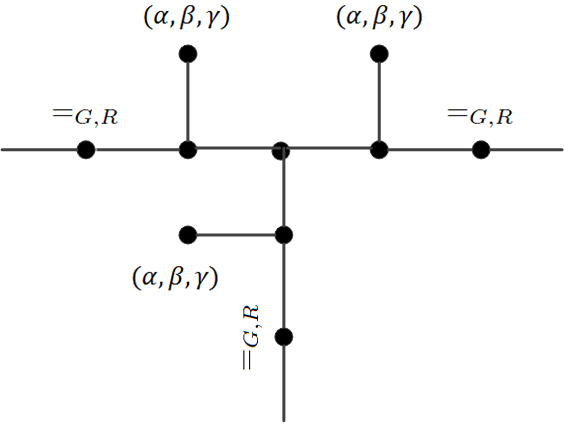
Figure 10: A ternary gadget.

We choose a unary $\mathbf{u}=(\alpha,\beta,0)$, such that the matrix form of $\langle\mathbf{u},\mathbf{F}\rangle$ is $M=\begin{bmatrix}w&x&y\\ x&z&iz\\ y&iz&-z\end{bmatrix}$, where $w=\alpha u+\beta t$, $x=\alpha t+\beta s$, $y=\alpha r+\beta is$ and $z=\alpha s+\beta$.

We wish to compute the signature of this construction, namely the ternary function $(M^{\otimes 3}\mathbf{F})^{*\rightarrow\{G,R\}}$ on domain size two. Consider the $2\times 3$ matrix $\begin{bmatrix}x&z&zi\\ y&zi&-z\end{bmatrix}$, which we decompose to $M_{1}M_{2}$, where $M_{1}=\begin{bmatrix}x&z&0\\ y&zi&0\end{bmatrix}$, and $M_{2}=\begin{bmatrix}1&0&0\\ 0&1&i\\ 0&0&0\end{bmatrix}$. Then $(M^{\otimes 3}\mathbf{F})^{*\rightarrow\{G,R\}}$ is $M_{1}^{\otimes 3}(M_{2}^{\otimes 3}\mathbf{F})$.

As $M_{2}$ has a separated domain form, $(M_{2}^{\otimes 3}\mathbf{F})^{*\rightarrow\{G,R\}}$ is identically 0, since these values are combinations of values from the bottom line $\mathbf{F}^{*\rightarrow\{G,R\}}$. Formally,

$$(M_{2}^{\otimes 3}\mathbf{F})^{*\rightarrow\{G,R\}}=\begin{bmatrix}0&1&i\\ 0&0&0\end{bmatrix}^{\otimes 3}\mathbf{F}=\begin{bmatrix}1&i\\ 0&0\end{bmatrix}^{\otimes 3}\begin{bmatrix}0&1&0\\ 0&0&1\end{bmatrix}^{\otimes 3}\mathbf{F}=\begin{bmatrix}1&i\\ 0&0\end{bmatrix}^{\otimes 3}\mathbf{F}^{*\rightarrow\{G,R\}}=\begin{bmatrix}1&i\\ 0&0\end{bmatrix}^{\otimes 3}\begin{bmatrix}1\\ i\end{bmatrix}^{\otimes 3}=\mathbf{0}.$$

To compute the other values of $M_{2}^{\otimes 3}\mathbf{F}$, we may set one input of $M_{2}^{\otimes 3}\mathbf{F}$ to $B$, which by the form of $M_{2}$ is the same as $M_{2}^{\otimes 2}(\mathbf{F}^{1=B})$. This can be computed as a matrix product $M_{2}\begin{bmatrix}u&t&r\\ t&s&is\\ r&is&-s\end{bmatrix}M_{2}^{\tt T}$, and the result is $\begin{bmatrix}u&t+ir&0\\ t+ir&0&0\\ 0&0&0\end{bmatrix}$. Thus the signature $M_{2}^{\otimes 3}\mathbf{F}$ is

			$u$
		$t+ir$		$0$
	$0$		$0$		$0$
$0$		$0$		$0$		$0$

which is

$$u\begin{bmatrix}1\\ 0\\ 0\end{bmatrix}^{\otimes 3}+(t+ir)\cdot\frac{1}{2}{\rm Sym}\left[\begin{bmatrix}1\\ 0\\ 0\end{bmatrix}^{\otimes 2}\otimes\begin{bmatrix}0\\ 1\\ 0\end{bmatrix}\right].$$

(The symmetrization Sym has six terms.)

Now we apply $M_{1}$, and get

$$u\begin{bmatrix}x\\ y\end{bmatrix}^{\otimes 3}+(t+ir)\cdot\frac{z}{2}{\rm Sym}\left[\begin{bmatrix}x\\ y\end{bmatrix}^{\otimes 2}\otimes\begin{bmatrix}1\\ i\end{bmatrix}\right].$$

If we can set $y=0$, with $x\neq 0$ and $z\not=0$, then this signature has the form $[a,b,0,0]$, with $b\not=0$. This defines a #P-hard problem on domain size two by Theorem 2.5. Similarly if we can set $x=0$, with $y\neq 0$ and $z\not=0$, then this signature has the form $[0,0,b,a]$, with $b\not=0$. This also defines a #P-hard problem by Theorem 2.5.

We will now show that if $s\not=0$, or if $s=0$ but $r\not=-it$, then we can indeed set $x$, $y$ and $z$ accordingly, and we will have proved the #P-hardness of Holant${}^{*}(\mathbf{F})$.

First suppose $s\not=0$. Since we have $r\not=it$, either $t\not=s^{2}$ or $r\not=is^{2}$. Set any $\alpha\not=0$. If $t\not=s^{2}$, then set $\beta=-\alpha t/s$ we get $x=\alpha t+\beta s=0$, and $y=\alpha r+\beta is=\alpha(r-it)\not=0$, and $z=\alpha s+\beta=\alpha(s^{2}-t)/s\not=0$. Similarly if $r\not=is^{2}$, then set $\beta=\alpha ir/s$ we get $y=\alpha r+\beta is=0$, and $x=\alpha t+\beta s=\alpha(t+ir)\not=0$, and $z=\alpha s+\beta=\alpha(s^{2}+ir)/s\not=0$.

Now suppose $s=0$. Then $x=\alpha t$, $y=\alpha r$ and $z=\beta$. We set $\beta=1/(t+ir)$ (recall that we have $r\not=it$). Then $(M^{\otimes 3}\mathbf{F})^{*\rightarrow\{G,R\}}$ is $\alpha^{2}\widehat{f}$, where

$$\widehat{f}=\alpha u\begin{bmatrix}t\\ r\end{bmatrix}^{\otimes 3}+\frac{1}{2}{\rm Sym}\left[\begin{bmatrix}t\\ r\end{bmatrix}^{\otimes 2}\otimes\begin{bmatrix}1\\ i\end{bmatrix}\right]$$ (26)

For $\alpha\not=0$, we can ignore the factor $\alpha^{2}$. When $u=0$ we can show the signature

$$f=\frac{1}{2}{\rm Sym}\left[\begin{bmatrix}t\\ r\end{bmatrix}^{\otimes 2}\otimes\begin{bmatrix}1\\ i\end{bmatrix}\right]=[3t^{2},t^{2}i+2tr,2tri+r^{2},3r^{2}i]$$

gives a #P-hard Holant^∗ problem as follows, by Theorem 2.5. First, $f$ is nondegenerate. After a holographic reduction $\begin{bmatrix}t&1\\ r&i\end{bmatrix}^{-1}$ this signature is $\tilde{f}=\frac{1}{2}{\rm Sym}\left[\begin{bmatrix}1\\ 0\end{bmatrix}^{\otimes 2}\otimes\begin{bmatrix}0\\ 1\end{bmatrix}\right]$. $f$ is degenerate iff $\tilde{f}$ is, and if this were the case, then $\tilde{f}=\begin{bmatrix}a\\ b\end{bmatrix}^{\otimes 3}$, for some $a$ and $b$. Taking $\langle\begin{bmatrix}1&0\end{bmatrix}^{\otimes 2},\tilde{f}\rangle$, we get $a=0$, and similarly, $\langle\begin{bmatrix}0&1\end{bmatrix}^{\otimes 2},\tilde{f}\rangle$ gives us $b=0$, a contradiction. Checking against the tractability criterion of Theorem 2.5, we find that Holant${}^{*}(f)$ is #P-hard, unless $t^{2}+r^{2}=0$. As $t+ir\not=0$, we get the only exceptional case $t-ir=0$.

Now we claim that the proof above also shows that for all $u$ not necessarily 0, the problem is #P-hard, assuming $t-ir\not=0$. This is because the conditions on degeneracy and on tractability are all expressed in terms polynomial equations on the entries of the signature. For any fixed $u$, if the conditions fail to be satisfied for $\widehat{f}$ at $\alpha=0$ (which is the same as when $u=0$ in (26), as has been shown), then the conditions also fail to be satisfied for some nonzero $\alpha$ sufficiently small. This shows that for all $u$ the problem Holant${}^{*}(\widehat{f})$, for some nonzero $\alpha$, is #P-hard. But for any nonzero $\alpha$, the problem Holant${}^{*}(\widehat{f})$ is equivalent to Holant${}^{*}((M^{\otimes 3}\mathbf{F})^{*\rightarrow\{G,R\}})$. Hence Holant${}^{*}(\mathbf{F})$ is #P-hard.

Now we suppose $s=0$, $t=ir$ and $u\neq 0$. As $t+ir\not=0$ we have $t\not=0$. We will use a slightly more complicated gadget as depicted in Figure 11, where the outer unary function is $\mathbf{u}_{1}=(1/t,1,0)$, and the inner unary function is $\mathbf{u}_{2}=(x,1,0)$.

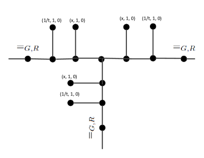
Figure 11: A ternary gadget.

We can calculate the binary function that is the linked chain of $\langle\mathbf{u}_{1},\mathbf{F}\rangle$ and $\langle\mathbf{u}_{2},\mathbf{F}\rangle$, and in matrix form it is

$$\begin{bmatrix}*&*&*\\ X&Z&-iZ\\ Y&-iZ&-Z\end{bmatrix}$$

where $X=x(u+2t)+t$, $Y=-iX+4ixt$ and $Z=xt$.

We can write $\begin{bmatrix}X&Z&-iZ\\ Y&-iZ&-Z\end{bmatrix}$ as $M_{1}M_{2}$, where

$$M_{1}=\begin{bmatrix}X&Z&0\\ Y&-iZ&0\end{bmatrix}\mbox{ and }M_{2}=\begin{bmatrix}1&0&0\\ 0&1&-i\\ 0&0&0\end{bmatrix}$$

It can be verified that $(M_{2})^{\otimes 3}\mathbf{F}$ is

			$u$
		$0$		$0$
	$0$		$0$		$0$
$8$		$0$		$0$		$0$

So the signature of the gadget is

$$(M_{1})^{\otimes 3}[(M_{2})^{\otimes 3}\mathbf{F}]=u\begin{bmatrix}X\\ Y\end{bmatrix}^{\otimes 3}+8\begin{bmatrix}Z\\ -iZ\end{bmatrix}^{\otimes 3}.$$

Since $X=x(u+2t)+t$, $Y=-iX+4ixt$ and $Z=xt$, we can always either set $X=0$ and $YZ\not=0$, or set $Y=0$ and $XZ\not=0$. (When $u+2t\not=0$, we can set $x=-t/(u+2t)\not=0$. When $u+2t=0$, then $X=t\not=0$, and we set $x=1/4$.) This proves #P-hardness given $u\neq 0$.

Finally, we suppose $s=0$, $t=ir$ and $u=0$. As $r\not=it$, we have $r,t\not=0$. $\mathbf{F}$ is

			$0$
		$ir$		$r$
	$0$		$0$		$0$
$1$		$i$		$-1$		$-i$

After a holographic reduction by the matrix $T=\left(\begin{array}[]{ccc}\sqrt{2}&0&0\\ 0&1&-i\\ 0&1&i\end{array}\right)$, $\mathbf{F}$ becomes $\mathbf{H}=T^{\otimes 3}\mathbf{F}=$

			$0$
		$0$		$4ri$
	$0$		$0$		$0$
$8$		$0$		$0$		$0$

Our problem Holant${}^{*}(\mathbf{F})$ can be restated as Holant$(\{=_{2}\}\cup\mathcal{U}|\{\mathbf{F}\}\cup\mathcal{U})$. The left hand side $=_{2}$ becomes ${(T^{-1})}^{\tt T}I_{3}T^{-1}$ which is a constant $1/2$ multiplied by $(\neq_{B;G,R})$ (see equation (18)). Holant${}^{*}(\mathbf{F})$ is holographic equivalent to Holant$(\{\neq_{B;G,R}\}\cup\mathcal{U}|\{\mathbf{H}\}\cup\mathcal{U})$.

We can realize on the right hand side $\langle\mathbf{H},(x,y,z)\rangle$, with a unary $(x,y,z)$, and on the left hand side $(\neq_{B;G,R})^{\otimes 3}\mathbf{H}=$

			$0$
		$4ri$		$0$
	$0$		$0$		$0$
$0$		$0$		$0$		$8$

It is easy to see that Holant$(\{(\neq_{B;G,R})^{\otimes 3}\mathbf{H}\}\cup\mathcal{U}\mid\{\langle\mathbf{H},(x,y,z)\rangle\}\cup\mathcal{U})$ can be simulated by, and therefore reducible to, Holant$(\{\neq_{G,R}\}\cup\mathcal{U}\mid\{\mathbf{H}\}\cup\mathcal{U})$.

Setting $x=0,y=\frac{1}{8},z=\frac{1}{4ri}$, we have the binary function which is an equality on $\{B,G\}$ and zero elsewhere, $\langle\mathbf{H},(x,y,z)\rangle=(=_{B,G})$. Then we can apply $(=_{B,G})$ to restrict $(\neq_{G,R})^{\otimes 3}\mathbf{H}$ to the subdomain $\{B,G\}$. Notice that $[(\neq_{G,R})^{\otimes 3}\mathbf{H}]^{*\rightarrow\{B,G\}}$ is $4ri[0,1,0,0]$, where $[0,1,0,0]$ is the Perfect Matching function of 3-regular graphs on the domain $\{B,G\}$. Hence we get a #P-hard problem.

5.6 $\mathbf{F}^{*\rightarrow\{G,R\}}=[0,0,0,0]$

We deal with the final case where $\mathbf{F}^{*\rightarrow\{G,R\}}$ is identically 0. The signature $\mathbf{F}$ is of the form

			$u$
		$t$		$r$
	$s$		$p$		$q$
$0$		$0$		$0$		$0$

Let $x$ and $y$ be such that $x^{2}+y^{2}=1$, then $H=\begin{bmatrix}x&y\\ y&-x\end{bmatrix}$ is an orthogonal matrix. Note that $y\neq\pm xi$. We will use $H$ to normalize $(s,p,q)$. This transformation happens in the domain $\{G,R\}$. Formally, we perform a transformation in the whole domain $\{B,G,R\}$ using the orthogonal matrix $\hat{H}=\begin{bmatrix}1&0&0\\ 0&x&y\\ 0&y&-x\end{bmatrix}$. Note that in $\hat{H}$ the domain $\{G,R\}$ is separated from $\{B\}$. $(\hat{H}^{\otimes 3}\mathbf{F})^{*\rightarrow\{G,R\}}$ is still [0,0,0,0]. This is because a value of $\hat{H}^{\otimes 3}\mathbf{F}$ under any assignment that is restricted to $\{G,R\}$ only, after the transformation $\hat{H}$, becomes a combination of values of $\mathbf{F}^{*\rightarrow\{G,R\}}$ under a tensor transformation of $H$, hence 0. To compute the rest of the signature of $\hat{H}^{\otimes 3}\mathbf{F}$, we may assign one input to $B$, and compute the binary signature $(\hat{H}^{\otimes 3}\mathbf{F})^{1=B}$ on $\{B,G,R\}$. By the form of $\hat{H}$ this is the same as $\hat{H}^{\otimes 2}(\mathbf{F}^{1=B})$. The matrix form is the matrix product $\hat{H}(\mathbf{F}^{1=B})\hat{H}^{\tt T}$, where the matrix form of $\mathbf{F}^{1=B}$ is $\begin{bmatrix}u&t&r\\ t&s&p\\ r&p&q\end{bmatrix}$. Thus $\hat{H}^{\otimes 3}\mathbf{F}$ is

			$u^{\prime}$
		$t^{\prime}$		$r^{\prime}$
	$s^{\prime}$		$p^{\prime}$		$q^{\prime}$
$0$		$0$		$0$		$0$

where

$$u^{\prime} = u$$

$$t^{\prime} = tx+ry$$

$$r^{\prime} = -rx+ty$$

$$s^{\prime} = sx^{2}+2pxy+qy^{2}$$

$$p^{\prime} = -px^{2}+(s-q)xy+py^{2}$$

$$q^{\prime} = qx^{2}-2pxy+sy^{2}$$

We easily verify that $(q^{\prime}-s^{\prime}\pm 2ip^{\prime})=(x\mp iy)^{2}(q-s\mp 2ip)$. Thus, for any given $x\not=\pm iy$, we have $q-s\mp 2ip\not=0$ iff $q^{\prime}-s^{\prime}\pm 2ip^{\prime}\not=0$.

1. Consider the case $s=p=q=0$. If $r=\pm it$, then $\mathbf{F}$ is in the third form of Theorem 3.1, since the isotropic $(0,1,\pm i)$ annihilates $\mathbf{F}$, namely $\langle(0,1,\pm i),\mathbf{F}\rangle=\mathbf{0}$. If $r\not=\pm it$, we can apply an orthogonal transformation $\hat{H}$ with $rx=ty$, such that $\mathbf{F}$ becomes

   			$u$
   		$t^{\prime}$		$0$
   	$0$		$0$		$0$
   $0$		$0$		$0$		$0$

   where $t^{\prime}=tx+ry\not=0$. This gives a #P-hard problem on the domain $\{B,G\}$.

   From now on not all $s,p,q=0$.

2. Suppose $p=0$. But either $s\not=0$ or $q\not=0$. Suppose $s\not=0$, by symmetry. We get the binary $\mathbf{F}^{1=G}$

   		$t$
   	$s$		$0$
   $0$		$0$		$0$

   which is effectively a domain two binary signature $[t,s,0]$. We can use this to interpolate $=_{B,G}$. Then it becomes a solved case before, by the substitution of $\{B,G\}$ for $\{G,R\}$. Note that $\mathbf{F}^{*\rightarrow\{B,G\}}$ is not identically 0.

   From now on $p\not=0$.

3. Suppose $q\not=s\pm 2ip$. We can set $y/x$ to be a solution to $Y^{2}+\frac{s-q}{p}Y-1=0$, such that $Y\not=\pm i$. Then $\hat{H}^{\otimes 3}\mathbf{F}$ has $p^{\prime}=0$. Note that $q^{\prime}\not=s^{\prime}\pm 2ip^{\prime}=s^{\prime}$, thus at least one of $s^{\prime}$ or $q^{\prime}\not=0$. Thus we have reduced this case to the previous case.

   From now on $q=s\pm 2ip$.

4. Suppose $p\not=0$, $q=s\pm 2ip$, and either $s=0$ or $q=0$. Then either $q=\pm 2ip$ or $s=\mp 2ip$. By symmetry assume $q=0$. We can get the binary $\mathbf{F}^{1=R}$

   		$r$
   	$p$		$0$
   $0$		$0$		$0$

   which is effectively a domain two binary signature $[r,p,0]$ on $\{B,G\}$. We can use this to interpolate $=_{B,G}$. Then it becomes a solved case before, by the substitution of $\{B,G\}$ for $\{G,R\}$, since $\mathbf{F}^{*\rightarrow\{B,G\}}$ is not identically 0.

   From now on both $s\not=0$ and $q\not=0$.

5. $s,p,q\not=0$, $q=s\pm 2ip$, but suppose $q\not=-s$. Setting $y/x=\frac{2p}{s}\mp i$, we can verify that this gives an orthogonal matrix $H$ such that $q^{\prime}=0$. This reduces to the previous case.

6. Finally we have $s,p,q\not=0$ and $q=s\pm 2ip=-s$. Then $p=\mp si$ and $(s,p,q)=s(1,\mp i,-1)$. We may normalize to $s=1$. We consider the case $(1,i,-1)$; the case $(1,-i,-1)$ is symmetric.

   If $r=it$, $\mathbf{F}$ is in the third form of Theorem 3.1, since $\langle(0,1,i),\mathbf{F}\rangle=\mathbf{0}$. Now we suppose $r\not=it$. We shall prove that the problem is #P-hard using the gadget in Figure 12.

   

   Figure 12: A ternary gadget.

   The unary $\mathbf{u}=(\alpha,\beta,\gamma)$ with $\alpha=1,\gamma=0$ is chosen such that the matrix form of $\langle\mathbf{u},\mathbf{F}\rangle$ is $M=\begin{bmatrix}z&x&y\\ x&1&i\\ y&i&-1\end{bmatrix}$, where $x=t+\beta,y=r+i\beta$. Note that the ratio of $x,y$ can be arbitrary, by choosing $\beta$.

   We wish to compute the signature of the gadget, which is the domain two signature of the ternary function $(M^{\otimes 3}\mathbf{F})^{*\rightarrow\{B,G\}}$. We can decompose the $2\times 3$ matrix $\begin{bmatrix}x&1&i\\ y&i&-1\end{bmatrix}$ as the product $M_{1}M_{2}$, where $M_{1}=\begin{bmatrix}x&1&0\\ y&i&0\end{bmatrix}$, and $M_{2}=\begin{bmatrix}1&0&0\\ 0&1&i\\ 0&0&0\end{bmatrix}$. Therefore we wish to compute $M_{1}^{\otimes 3}(M_{2}^{\otimes 3}\mathbf{F})$.

   As $M_{2}$ has a separated domain form, $(M_{2}^{\otimes 3}\mathbf{F})^{*\rightarrow\{G,R\}}$ is identically 0, since these values are combinations of values from the bottom line $\mathbf{F}^{*\rightarrow\{G,R\}}$ by a tensor transformation. To compute the other values of $M_{2}^{\otimes 3}\mathbf{F}$, we may set one input of $M_{2}^{\otimes 3}\mathbf{F}$ to $B$, which by the form of $M_{2}$ is the same as $M_{2}^{\otimes 2}(\mathbf{F}^{1=B})$. This can be computed by a matrix product and the result is $\begin{bmatrix}u&t+ir&0\\ t+ir&0&0\\ 0&0&0\end{bmatrix}$. Thus the signature $M_{2}^{\otimes 3}\mathbf{F}$ is

   			$u$
   		$t+ir$		$0$
   	$0$		$0$		$0$
   $0$		$0$		$0$		$0$

   which is

   $$u\begin{bmatrix}1\\ 0\\ 0\end{bmatrix}^{\otimes 3}+(t+ir)\cdot\frac{1}{2}{\rm Sym}\left[\begin{bmatrix}1\\ 0\\ 0\end{bmatrix}^{\otimes 2}\otimes\begin{bmatrix}0\\ 1\\ 0\end{bmatrix}\right].$$

   (The symmetrization has six terms.)

   Now we apply $M_{1}$, and get

   $$u\begin{bmatrix}x\\ y\end{bmatrix}^{\otimes 3}+(t+ir)\cdot\frac{1}{2}{\rm Sym}\left[\begin{bmatrix}x\\ y\end{bmatrix}^{\otimes 2}\otimes\begin{bmatrix}1\\ i\end{bmatrix}\right].$$

   If we set $\beta=ir$, then $x=t+ir\not=0$ and $y=0$. This signature is $[(u+1)x^{3},ix^{3},0,0]$. Since $x\not=0$ this defines a #P-hard problem on domain size two by Theorem 2.5.

References

- [1] Ali Al-Bashabsheh and Yongyi Mao. Normal factor graphs and holographic transformations. IEEE Transactions on Information Theory, 57(2):752–763, 2011.
- [2] Ali Al-Bashabsheh, Yongyi Mao, and Pascal O. Vontobel. Normal factor graphs: A diagrammatic approach to linear algebra. In Alexander Kuleshov, Vladimir Blinovsky, and Anthony Ephremides, editors, ISIT, pages 2178–2182. IEEE, 2011.
- [3] R.J. Baxter. Exactly solved models in statistical mechanics. Academic press London, 1982.
- [4] A. Bulatov, M. Dyer, L.A. Goldberg, M. Jalsenius, and D. Richerby. The complexity of weighted boolean #CSP with mixed signs. Theoretical Computer Science, 410(38-40):3949–3961, 2009.
- [5] Andrei A. Bulatov. A dichotomy theorem for constraint satisfaction problems on a 3-element set. J. ACM, 53(1):66–120, 2006.
- [6] Andrei A. Bulatov. The complexity of the counting constraint satisfaction problem. In Luca Aceto, Ivan Damgård, Leslie Ann Goldberg, Magnús M. Halldórsson, Anna Ingólfsdóttir, and Igor Walukiewicz, editors, ICALP (1), volume 5125 of Lecture Notes in Computer Science, pages 646–661. Springer, 2008.
- [7] Andrei A. Bulatov and Víctor Dalmau. Towards a dichotomy theorem for the counting constraint satisfaction problem. In FOCS, pages 562–571. IEEE Computer Society, 2003.
- [8] Andrei A. Bulatov and Martin Grohe. The complexity of partition functions. Theor. Comput. Sci., 348(2-3):148–186, 2005.
- [9] Jin-Yi Cai and Xi Chen. Complexity of counting csp with complex weights. In Howard J. Karloff and Toniann Pitassi, editors, STOC, pages 909–920. ACM, 2012.
- [10] Jin-Yi Cai, Xi Chen, and Pinyan Lu. Graph homomorphisms with complex values: A dichotomy theorem. In Samson Abramsky, Cyril Gavoille, Claude Kirchner, Friedhelm Meyer auf der Heide, and Paul G. Spirakis, editors, ICALP (1), volume 6198 of Lecture Notes in Computer Science, pages 275–286. Springer, 2010.
- [11] Jin-Yi Cai, Xi Chen, and Pinyan Lu. Non-negatively weighted #CSP: An effective complexity dichotomy. In IEEE Conference on Computational Complexity, pages 45–54, 2011.
- [12] Jin-Yi Cai, Sangxia Huang, and Pinyan Lu. From holant to #CSP and back: Dichotomy for holant problems. In Otfried Cheong, Kyung-Yong Chwa, and Kunsoo Park, editors, ISAAC (1), volume 6506 of Lecture Notes in Computer Science, pages 253–265. Springer, 2010.
- [13] Jin-Yi Cai, Pinyan Lu, and Mingji Xia. Holographic algorithms by fibonacci gates and holographic reductions for hardness. In FOCS ’08: Proceedings of the 49th Annual IEEE Symposium on Foundations of Computer Science, Washington, DC, USA, 2008. IEEE Computer Society.
- [14] Jin-Yi Cai, Pinyan Lu, and Mingji Xia. Holant problems and counting CSP. In Michael Mitzenmacher, editor, STOC, pages 715–724. ACM, 2009.
- [15] Jin-Yi Cai, Pinyan Lu, and Mingji Xia. Computational complexity of holant problems. SIAM J. Comput., 40(4):1101–1132, 2011.
- [16] Jin-Yi Cai, Pinyan Lu, and Mingji Xia. Dichotomy for holant∗ problems of boolean domain. In SODA ’11: Proceedings of the nineteenth annual ACM-SIAM symposium on Discrete algorithms, 2011.
- [17] Nadia Creignou and Miki Hermann. Complexity of generalized satisfiability counting problems. Inf. Comput., 125(1):1–12, 1996.
- [18] C. T. J. Dodson and T. Poston. Tensor Geometry. Graduate Texts in Mathematics 130. Springer-Verlag, New York, 1991.
- [19] Martin E. Dyer, Leslie Ann Goldberg, and Mark Jerrum. The complexity of weighted boolean csp. SIAM J. Comput., 38(5):1970–1986, 2009.
- [20] M.E. Dyer and C. Greenhill. The complexity of counting graph homomorphisms. In Proceedings of the 9th International Conference on Random Structures and Algorithms, pages 260–289, 2000.
- [21] M.E. Dyer and D.M. Richerby. On the complexity of #CSP. In Proceedings of the 42nd ACM symposium on Theory of computing, pages 725–734, 2010.
- [22] M.E. Dyer and D.M. Richerby. The #CSP dichotomy is decidable. In Proceedings of the 28th Symposium on Theoretical Aspects of Computer Science, 2011.
- [23] T. Feder and M.Y. Vardi. The computational structure of monotone monadic SNP and constraint satisfaction: A study through Datalog and group theory. SIAM Journal on Computing, 28(1):57–104, 1998.
- [24] R.P. Feynman. Feynman lectures on physics. Addison Wesley Longman, 1970.
- [25] M. Freedman, L. Lovász, and A. Schrijver. Reflection positivity, rank connectivity, and homomorphism of graphs. J. AMS, 20:37–51, 2007.
- [26] Leslie Ann Goldberg, Martin Grohe, Mark Jerrum, and Marc Thurley. A complexity dichotomy for partition functions with mixed signs. SIAM J. Comput., 39(7):3336–3402, 2010.
- [27] Leslie Ann Goldberg and Mark Jerrum. Approximating the partition function of the ferromagnetic potts model. In Proceedings of the 37th international colloquium conference on Automata, languages and programming, ICALP ’10, pages 396–407, Berlin, Heidelberg, 2010. Springer-Verlag.
- [28] Leslie Ann Goldberg, Mark Jerrum, and Mike Paterson. The computational complexity of two-state spin systems. Random Struct. Algorithms, 23(2):133–154, 2003.
- [29] Heng Guo, Pinyan Lu, and Leslie G. Valiant. The complexity of symmetric boolean parity holant problems - (extended abstract). In Luca Aceto, Monika Henzinger, and Jiri Sgall, editors, ICALP (1), volume 6755 of Lecture Notes in Computer Science, pages 712–723. Springer, 2011.
- [30] Sangxia Huang and Pinyan Lu. A dichotomy for real weighted holant problems. to appear at CCC 2012.
- [31] E. Ising. Beitrag zur theorie des ferromagnetismus. Zeitschrift für Physik A Hadrons and Nuclei, 31(1):253–258, 1925.
- [32] Mark Jerrum and Alistair Sinclair. Polynomial-time approximation algorithms for the ising model. SIAM Journal on Computing, 22(5):1087–1116, 1993.
- [33] G. David Forney Jr. Codes on graphs: Normal realizations. IEEE Transactions on Information Theory, 47(2):520–548, 2001.
- [34] G. David Forney Jr. and Pascal O. Vontobel. Partition functions of normal factor graphs. CoRR, abs/1102.0316, 2011.
- [35] P. W. Kasteleyn. The statistics of dimers on a lattice. Physica, 27:1209–1225, 1961.
- [36] Richard E. Ladner. On the structure of polynomial time reducibility. J. ACM, 22(1):155–171, 1975.
- [37] L. Lovász. Operations with structures. Acta Math. Hung., 18:321–328, 1967.
- [38] B.M. McCoy and T.T. Wu. The two-dimensional Ising model. Harvard University Press Cambridge, 1973.
- [39] T.J. Schaefer. The complexity of satisfiability problems. In Proceedings of the 10th annual ACM symposium on Theory of computing, pages 216–226, 1978.
- [40] N. H. Scott. A new canonical form for complex symmetric matrices. Proceedings: Mathematical and Physical Sciences, 441(1913):pp. 625–640, 1993.
- [41] H. N. V. Temperley and M. E. Fisher. Dimer problem in statistical mechanics c an exact result. Philosophical Magazine, 6:1061 C 1063, 1961.
- [42] Leslie G. Valiant. Accidental algorthims. In FOCS ’06: Proceedings of the 47th Annual IEEE Symposium on Foundations of Computer Science, pages 509–517, Washington, DC, USA, 2006. IEEE Computer Society.
- [43] Leslie G. Valiant. Holographic algorithms. SIAM J. Comput., 37(5):1565–1594, 2008.