Abstract

We consider mean curvature flow of $n$-dimensional surface clusters. At $(n-1)$-dimensional triple junctions an angle condition is required which in the symmetric case reduces to the well-known 120 degree angle condition. Using a novel parametrization of evolving surface clusters and a new existence and regularity approach for parabolic equations on surface clusters we show local well-posedness by a contraction argument in parabolic Hölder spaces.

Key words: Mean curvature flow, triple lines, local existence result, parabolic Hölder theory, free boundary problem.

AMS-Classification: 53C44, 35K55, 35R35, 58J35.

1 Introduction

Motion by mean curvature for evolving hypersurfaces in $\mathbb{R}^{n+1}$ is given by

$$V=H\,,$$

where $V$ is the normal velocity and $H$ is the mean curvature of the evolving surface. Mean curvature flow for closed surfaces is the $L^{2}$-gradient flow of the area functional and many results for this flow have been established over the last 30 years, see e.g. Huisken [19], Gage and Hamilton [14], Ecker [9], Giga [17], Mantegazza [24] and the references therein.

Less is known for mean curvature flow of surfaces with boundaries. In the simplest cases one either prescribes fixed Dirichlet boundary data or one requires that surfaces meet a given surface with a $90$ degree angle. The last situation can be interpreted as the $L^{2}$-gradient flow of area taking the side constraint into account that the boundary of the surface has to lie on a given external surface. A setting where the surface is given as a graph was studied by Huisken [20], who could also analyze the long time behaviour in the case where the evolving surface was given as the graph over a fixed domain. Local well-posedness for general geometries was shown by Stahl [29] who was also able to formulate a continuation criterion. In addition he showed that surfaces converge asymptotically to a half sphere before they vanish.

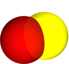
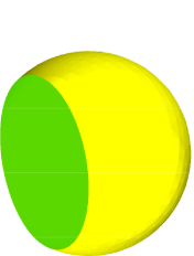
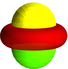
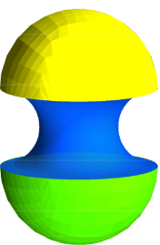
Figure 1: A surface cluster consisting of three hypersurfaces with boundary and one triple line on the left; and a surface cluster with four hypersurfaces, where the topology of the individual surfaces is not the same for all on the right; taken from [3].

Much less is known about the gradient flow dynamics for surface clusters. In this case hypersurfaces $\Gamma^{1},\dots,\Gamma^{N}$ in $\mathbb{R}^{n+1}$ with boundaries $\partial\Gamma^{1},\dots,\partial\Gamma^{N}$ meet at $(n-1)$-dimensional triple junctions, see e.g. Figure 1. Here, boundary conditions at the triple junction which can be derived variationally have to be described. In what follows we briefly discuss how to derive these boundary conditions. We define the weighted surface free energy

$$\mathcal{F}(\Gamma):=\sum^{N}_{i=1}\int\limits_{\Gamma^{i}}\gamma^{i}d\mathcal{H}^{n}$$

for a given surface cluster $\Gamma=(\Gamma^{1},\dots,\Gamma^{N})$ (and constant surface energy densities $\gamma_{i}>0$, $i=1,\ldots,N$) and consider a given smooth vector field

$$\zeta:\mathbb{R}^{n+1}\to\mathbb{R}^{n+1}\,.$$

Then we can define a variation $\Gamma(\varepsilon)$ of $\Gamma$ in the direction $\zeta$ via

$$\Gamma^{i}(\varepsilon)=\{x+\varepsilon\zeta(x)\mid x\in\Gamma^{i}\}\,.$$

A transport theorem now gives

$$\frac{d}{d\varepsilon}\int\limits_{\Gamma^{i}(\varepsilon)}1d\mathcal{H}^{n}=-\int\limits_{\Gamma^{i}(\varepsilon)}V^{i}H^{i}d\mathcal{H}^{n}+\int\limits_{\partial\Gamma^{i}(\varepsilon)}v^{i}d\mathcal{H}^{n-1}\,,$$

where $V^{i}$ is the normal velocity and $H^{i}$ is the mean curvature of $\Gamma^{i}$. In addition $v^{i}$ is the outer conormal velocity of the surface, i.e. we have $v^{i}=\langle\zeta,\nu^{i}\rangle$, where $\nu^{i}$ is the outer unit conormal of $\partial\Gamma^{i}$ (for details we refer to Garcke, Wieland [16] and Depner, Garcke [8]).

The first variation of $\mathcal{F}$ is now given by

$$\frac{d}{d\varepsilon}\mathcal{F}(\Gamma(\varepsilon))=\sum_{i}\int_{\Gamma^{i}(\varepsilon)}\left(-\gamma^{i}V^{i}H^{i}\right)d\mathcal{H}^{n}+\sum_{i}\int_{\partial\Gamma^{i}(\varepsilon)}\gamma^{i}v^{i}d\mathcal{H}^{n-1}$$

and hence a suitably weighted $L^{2}$-gradient flow is given by

$$V^{i}=\beta^{i}H^{i} \mbox{on }\Gamma^{i}\mbox{ and}$$ (1.1)

$$\sum^{3}_{i=1}\gamma^{i}\nu^{i}=0 \mbox{at triple junctions}.$$ (1.2)

We remark that the last condition reduces to a $120^{\circ}$ angle condition in the case that all $\gamma_{i}$’s are equal.

Local well-posedness for curves in the plane has been shown by Bronsard and Reitich [6] in a $C^{2+\alpha,1+\frac{\alpha}{2}}$ setting using parabolic regularity theory and a fixed point argument (for a typical solution see Figure 2). Kinderlehrer and Liu [21] derived global existence of a planar network of grain boundaries driven by curvature close to an equilibrium. Mantegazza, Novaga and Tortorelli [25] were able to establish continuation criteria and Schnürer et al. [27] and Bellettini and Novaga [4] considered the asymptotic behaviour of lens-shaped geometries. We remark that all of these results are restricted to the planar case.

$\underset{\mbox{equal area}}{\includegraphics[angle={-90},width=159.3382pt]{MC2}}$   $\underset{\mbox{non-equal area}}{\includegraphics[angle={-90},width=159.3382pt]{MC3}}$

Figure 2: Mean curvature flow of a double bubble in the plane, see [3] for results in $\mathbb{R}^{3}$.

The higher dimensional situation is much more involved as the triple junction now is at least one-dimensional and a tangential degree of freedom arises at the triple junction. In addition, all mathematical descriptions of the problem result in formulations which lead to a free boundary problem. Only recently, Freire [13] was able to show local well-posedness in the case of graphs. Of course most situations cannot be represented as graphs. We use a new parametrization of surface clusters introduced in Depner and Garcke [8] to state the problem (1.1), (1.2) as a system of non-local, quasilinear parabolic partial differential equations of second order. The PDEs are defined on a surface cluster and are non-trivially coupled at the junctions. To simplify the presentation, we will now stick to the situation of three surfaces meeting at one common triple junction. But we remark that generalizations of our approach to more general surface clusters are possible as long as different triple junctions do not meet. Of course this can happen for soap bubble clusters, see Taylor [30] and Morgan [26]. In addition we want to remark that in the situation on the left in Figure 1 it is in principle possible to use one global parametrization for all three evolving hypersurfaces. In this case we would get a system of PDEs on one reference configuration. Due to the topological restrictions this is not possible any more in the situation on the right in Figure 1. But since we only use local parametrizations, our method works also in this case.

We hence look for families of evolving hypersurfaces $\Gamma^{i}(t)\subset\mathbb{R}^{n+1}$ ($i=1,2,3$) governed by the mean curvature flow, which is weighted by $\beta^{i}>0$ ($i=1,2,3$). These hypersurfaces meet at their boundaries as follows

$$\partial\Gamma^{1}(t)=\partial\Gamma^{2}(t)=\partial\Gamma^{3}(t)\,(=:\Sigma(t)),$$

which is an $(n-1)$-dimensional manifold. Also, the angles between hypersurfaces are prescribed. More precisely, we consider

$$\left\{\begin{array}[]{l}V^{i}=\beta^{i}H^{i}\,\,\ \mbox{on}\,\,\ \Gamma^{i}(t),\ t\in[0,T]\,\ (i=1,2,3),\\[2.84544pt] \angle(\Gamma^{i}(t),\Gamma^{j}(t))=\theta^{k}\,\,\ \mbox{on}\,\ \Sigma(t),\ t\in[0,T],\\[2.84544pt] \qquad((i,j,k)=(1,2,3),\,(2,3,1),\,(3,1,2)),\\[2.84544pt] \Gamma^{i}(t)|_{t=0}=\Gamma^{i}_{0}\,\ (i=1,2,3),\end{array}\right.$$ (1.7)

where $\Gamma^{i}_{0}$ ($i=1,2,3$) are given initial hypersurfaces, which meet at their boundary, i.e. $\partial\Gamma_{0}^{1}=\partial\Gamma_{0}^{2}=\partial\Gamma_{0}^{3}\,(=:\Sigma_{0})$, and fulfill the angle conditions as above. Here, $V^{i}$ and $H^{i}$ are the normal velocity and mean curvature of $\Gamma^{i}(t)$, respectively.

In (1.7), $\theta^{1},\theta^{2}$ and $\theta^{3}$ are given contact angles with $0<\theta^{i}<\pi$, which fulfill $\theta^{1}+\theta^{2}+\theta^{3}=2\pi$ and Young’s law

$$\frac{\sin\theta^{1}}{\gamma^{1}}=\frac{\sin\theta^{2}}{\gamma^{2}}=\frac{\sin\theta^{3}}{\gamma^{3}}\;.$$ (1.8)

Let $\nu^{i}(\cdot,t)$ ($i=1,2,3$) be the outer conormals at $\partial\Gamma^{i}(t)$. Then, introducing the angle conditions as in (1.7), one can show that (1.8) is equivalent to

$$\gamma^{1}\nu^{1}(\cdot,t)+\gamma^{2}\nu^{2}(\cdot,t)+\gamma^{3}\nu^{3}(\cdot,t)=0\,\,\ \mbox{on}\,\,\ \Sigma(t),$$ (1.9)

which is the condition (1.2) stated above. To choose appropriate normals $N^{i}(\cdot,t)$ of $\Gamma^{i}(t)$, we observe that due to the appearance of a triple junction $\Sigma(t)$ the six vectors $N^{i}(\cdot,t)$, $\nu^{i}(\cdot,t)$, $i=1,2,3$ on $\Sigma(t)$ all lie in a two-dimensional space, namely the orthogonal complement $\left(T_{\sigma}\Sigma(t)\right)^{\perp}$ of the triple junction. In this two-dimensional space we choose an oriented basis and a corresponding counterclockwise rotation $R$ around $90$ degree. Then we set

$$N^{i}(\cdot,t):=R\nu^{i}(\cdot,t)\quad\mbox{ on }\;\Sigma(t)$$

and extend these normals by continuity to all of $\Gamma^{i}(t)$. Then we can write instead of (1.9)

$$\gamma^{1}N^{1}(\cdot,t)+\gamma^{2}N^{2}(\cdot,t)+\gamma^{3}N^{3}(\cdot,t)=0\,\,\ \mbox{on}\,\,\ \Sigma(t).$$ (1.10)

In the following the angle conditions at the triple line are written as

$$\langle N^{i}(\cdot,t),N^{j}(\cdot,t)\rangle=\cos\theta^{k}$$ (1.11)

on $\Sigma(t)$ for $(i,j,k)=(1,2,3)$, $(2,3,1)$, and $(3,1,2)$. Here and hereafter, $\langle\,\cdot\,,\,\cdot\,\rangle$ means the inner product in ${\mathbb{R}}^{n+1}$.

We are able to show the following result (for a precise formulation of the result we refer to Section 5):

Main result.
Let $(\Gamma^{1}_{0},\Gamma^{2}_{0},\Gamma^{3}_{0})$ be a $C^{2+\alpha}$ surface cluster with a $C^{2+\alpha}$ triple junction curve $\gamma$. We assume the compatibility conditions

• $(\Gamma^{1}_{0},\Gamma^{2}_{0},\Gamma^{3}_{0})$ fulfill the angle conditions,

• $\gamma^{1}\beta^{1}H^{1}_{0}+\gamma^{2}\beta^{2}H^{2}_{0}+\gamma^{3}\beta^{3}H^{3}_{0}=0$ on the triple line $\partial\Gamma^{1}_{0}=\partial\Gamma^{2}_{0}=\partial\Gamma^{3}_{0}$.

Then there exists a local $C^{2+\alpha,1+\frac{\alpha}{2}}$ solution of

$$V^{i}=H^{i}\,\,\ +\,\,\ \mbox{angle conditions},$$

with initial data $(\Gamma^{1}_{0},\Gamma^{2}_{0},\Gamma^{3}_{0})$.

The idea of the proof is as follows: First we study the linearized problem around a reference configuration with energy methods (this is non-trivial as the system is defined on a surface cluster). Then we show local $C^{2+\alpha,1+\frac{\alpha}{2}}$-regularity of the solutions to the linearized problem. In order to apply classical regularity theory close to the triple junction, we parametrize the cluster locally over one fixed reference domain and check the Lopatinskii-Shapiro condition for the resulting spatially localized system on the flat reference domain directly and for convenience with an energy argument. Finally we use a fixed point argument in $C^{2+\alpha,1+\frac{\alpha}{2}}$ which is non-trivial as the overall system is non-local. In this context ideas of Baconneau and Lunardi [2] are useful.

We remark that we do not need the initial surfaces $\Gamma^{i}_{0}$ to be of class $C^{3+\alpha}$ as in [2] since we linearize around smooth enough reference hypersurfaces, which are close enough to $\Gamma^{i}_{0}$ in the $C^{2+\alpha}$-norm.

We also remark that the overall problem has a structure similar as free boundary problems. This is due to the fact that at the triple junction a motion of the surface cluster in conormal direction is necessary. When formulating the evolution on a fixed reference configuration, we need to take care of the conormal velocity which results in a highly nonlinear nonlocal evolution problem similar as in several free boundary problems, see e.g. Escher and Simonett [11] or Baconneau and Lunardi [2]. In our context an additional difficulty arises due to the fact that three surfaces who all have a conormal velocity meet at the triple junction. The connection to free boundary problems is more apparent in the graph case which has been considered by Freire [13].

2 PDE formulation

2.1 Parametrization of surface clusters

Let us describe $\Gamma^{i}(t)$ with the help of functions $\rho^{i}:\Gamma^{i}_{\ast}\times[0,T]\to\mathbb{R}$ as graphs over some fixed compact reference hypersurfaces $\Gamma^{i}_{\ast}$ ($i=1,2,3$) of class $C^{3+\alpha}$ for some $0<\alpha<1$ with boundary $\partial\Gamma^{i}_{\ast}$. These are supposed to have a common boundary

$$\partial\Gamma^{1}_{\ast}=\partial\Gamma^{2}_{\ast}=\partial\Gamma^{3}_{\ast}\,(=:\Sigma_{\ast})$$ (2.1)

and fulfill the angle conditions from (1.7). As above, we introduce notation such that the outer conormals $\nu^{i}_{\ast}$ at $\partial\Gamma^{i}_{\ast}$ fulfill

$$\gamma^{1}\nu^{1}_{\ast}+\gamma^{2}\nu^{2}_{\ast}+\gamma^{3}\nu^{3}_{\ast}=0\quad\mbox{on }\;\Sigma_{\ast}\;,$$

and the normals $N^{i}_{\ast}$ of $\Gamma^{i}_{\ast}$ are chosen such that

$$\gamma^{1}N^{1}_{\ast}+\gamma^{2}N^{2}_{\ast}+\gamma^{3}N^{3}_{\ast}=0\quad\mbox{on }\;\Sigma_{\ast}\;.$$ (2.2)

Note that we do not assume $\Gamma^{i}_{\ast}$ to be a stationary solution of (1.7), that is the mean curvature of $\Gamma^{i}_{\ast}$ can be arbitrary.

Let $F^{i}\,:\,\Omega^{i}\rightarrow\mathbb{R}^{n+1}$ be a local parametrization with $F^{i}(\Omega^{i})\subset\Gamma_{*}^{i}$ where $\Omega^{i}$ is either an open subset of $\mathbb{R}^{n}$ or $B^{+}(0)=\{x\in\mathbb{R}^{n}\,|\,|x|<1r\,,\;x_{n}\geq 0\}$ in the case that we parametrize around a boundary point. For $\sigma\in\Gamma_{*}^{i}$, we set $F^{-1}(\sigma)=(x_{1}(\sigma),\ldots,x_{n}(\sigma))\in\mathbb{R}^{n}$. Here and hereafter, for simplicity, we use the notation

$$w(\sigma)=w(x_{1},\ldots,x_{n})\quad(\sigma\in\Gamma_{*}^{i})\,,$$

i.e. we omit the parametrization. In particular, we set $\partial_{l}w:=\partial_{x_{l}}(w\circ F)$.

To parametrize a hypersurface close to $\Gamma_{\ast}^{i}$, we define the mapping through

$$\Psi^{i}\,:\,\Gamma^{i}_{\ast}\times(-\varepsilon,\varepsilon)\times(-\delta,\delta)\rightarrow \ \mathbb{R}^{n+1}\;,$$ (2.3)

$$(\sigma,w,r)\mapsto \ \Psi^{i}(\sigma,w,r):=\sigma+w\,N^{i}_{\ast}(\sigma)+r\,\tau^{i}_{\ast}(\sigma)\;,$$

where $\tau^{i}_{\ast}$ is a tangential vector field on $\Gamma^{i}_{\ast}$ with support in a neighbourhood of $\partial\Gamma^{i}_{\ast}$, which equals the conormal $\nu^{i}_{\ast}$ at $\partial\Gamma^{i}_{\ast}$. The index $i$ has range $1,2,3$.

For $i=1,2,3$ and functions

$$\rho^{i}\,:\,\Gamma^{i}_{\ast}\times[0,T]\rightarrow(-\varepsilon,\varepsilon)\,,\quad\mu^{i}\,:\,\Sigma_{\ast}\times[0,T]\rightarrow(-\delta,\delta)$$

we define the mappings $\Phi^{i}=\Phi^{i}_{\rho^{i},\mu^{i}}$ (we often omit the subscript $(\rho^{i},\mu^{i}$) for shortness) through

$$\Phi^{i}:\Gamma^{i}_{\ast}\times[0,T]\rightarrow \ \mathbb{R}^{n+1}\;,\quad\Phi^{i}(\sigma,t):=\Psi^{i}(\sigma,\rho^{i}(\sigma,t),\mu^{i}(\operatorname{pr}^{i}(\sigma),t))\,.$$

Herein $\operatorname{pr}^{i}:\Gamma^{i}_{\ast}\to\partial\Gamma^{i}_{\ast}$ is defined such that $\operatorname{pr}^{i}(\sigma)\in\partial\Gamma^{i}_{\ast}$ is the point on $\partial\Gamma^{i}_{\ast}$ with shortest distance on $\Gamma^{i}_{\ast}$ to $\sigma$. We remark here that $\operatorname{pr}^{i}$ is well-defined and smooth close to $\partial\Gamma^{i}_{\ast}$. Note that we need this mapping just in a (small) neighbourhood of $\partial\Gamma^{i}_{\ast}$, because it is used in the product $\mu^{i}(\operatorname{pr}^{i}(\sigma),t)\,\tau^{i}_{\ast}(\sigma)$, where the second term is zero outside a (small) neighbourhood of $\partial\Gamma^{i}_{\ast}$. For small $\varepsilon,\delta>0$ and fixed $t$ we set

$$(\Phi^{i})_{t}\,:\,\Gamma^{i}_{\ast}\rightarrow\mathbb{R}^{n+1},\,\,\quad(\Phi^{i})_{t}(\sigma):=\Phi^{i}(\sigma,t)\,,$$

and finally we define new hypersurfaces through

$$\Gamma_{\rho^{i},\mu^{i}}(t):=\mbox{image}((\Phi^{i})_{t})\,.$$ (2.4)

We observe that for $\rho^{i}\equiv 0$ and $\mu^{i}\equiv 0$ the resulting surface is simply $\Gamma_{\rho^{i}\equiv 0,\mu^{i}\equiv 0}(t)=\Gamma^{i}_{\ast}$ for every $t$.

Remark 2.1.

We remark that for $\rho^{i}\in C^{2}(\Gamma^{i}_{\ast})$ and $\mu^{i}\in C^{2}(\Sigma_{\ast})$ small enough in the $C^{1}(\Gamma^{i}_{\ast})$- resp. $C^{1}(\Sigma_{\ast})$-norm the mapping $(\Phi^{i})_{t}$ is a local $C^{2}$-diffeomorphism onto its image.

In fact, omitting the time variable $t$ and the index $i$ for the moment, choosing a local parametrization and using the above abbreviations we calculate

$$\partial_{l}\Phi =\partial_{l}q+\partial_{l}\rho\,N_{\ast}+\rho\partial_{l}N_{\ast}+\partial_{l}(\mu\circ\operatorname{pr})\,\tau_{\ast}+(\mu\circ\operatorname{pr})\partial_{l}\tau_{\ast}\,.$$

A rather lengthy, but elementary calculation for $g_{lk}=\langle\partial_{l}\Phi,\partial_{k}\Phi\rangle$ gives

$$g_{lk} =(g_{\ast})_{lk}+P_{lk}(\rho,(\mu\circ\operatorname{pr}),\nabla\rho,\nabla(\mu\circ\operatorname{pr}))\,,$$

where $P_{lk}$ is a polynomial with $P_{lk}(0)=0$. With the help of the Leibniz formula for the determinant we can then derive

$$g=\det\left((g_{lk})_{l,k=1,\ldots,n}\right)=g_{\ast}+P(\rho,(\mu\circ\operatorname{pr}),\nabla\rho,\nabla(\mu\circ\operatorname{pr}))\,,$$

where $P$ is a polynomial with $P(0)=0$. Since $g_{\ast}>0$ we conclude that for $\rho$ and $\mu$ small enough in the $C^{1}$-norms also $g$ is positive. Together with the fact that $(g_{lk})_{l,k=1,\ldots,n}$ is positive semi-definite due to

$$\sum_{l,k=1}^{n}\xi_{l}g_{lk}\xi_{k}=\sum_{l,k=1}^{n}\xi_{l}\langle\partial_{l}\Phi,\partial_{k}\Phi\xi_{k}\rangle=\left|\sum_{l=1}^{n}\xi_{l}\partial_{l}\Phi\right|^{2}\geq 0\;\mbox{ for all }\,\xi\in\mathbb{R}^{n}\,,$$ (2.5)

we conclude the property that $(g_{lk})_{l,k=1,\ldots,n}$ is even positive definite. Hence we obtain a strict inequality in (2.5), whenever $\xi\neq 0$ and we conclude that $\partial_{1}\Phi,\ldots,\partial_{n}\Phi$ are linearly independent, which means that the differential $d\Phi(\sigma)$ has full rank.

Finally with the help of the inverse function theorem we conclude that $(\Phi^{i})_{t}$ is a local diffeomorphism and the image $\Gamma_{i}(t)$ has metric tensor $(g_{lk})_{l,k=1,\ldots,n}$.

In the definition of $\Psi^{i}$ we allow at the triple junction for a movement in normal and tangential direction, and hence there are enough degrees of freedom to formulate the condition, that the hypersurfaces $\Gamma_{i}(t)$ meet in one triple junction $\Sigma(t)$ at their boundary, through

$$\Phi^{1}(\sigma,t)=\Phi^{2}(\sigma,t)=\Phi^{3}(\sigma,t)\quad\mbox{for }\;\sigma\in\Sigma_{\ast}\;,\ t\geq 0\,.$$ (2.6)

We rewrite these equations in the following lemma, which was shown in Depner and Garcke [8].

Lemma 2.2.

Equivalent to the equations (2.6) are the following conditions

$$\left\{\begin{array}[]{cll}(i)&\gamma^{1}\rho^{1}+\gamma^{2}\rho^{2}+\gamma^{3}\rho^{3}=0&\mbox{on }\,\Sigma_{\ast}\,,\\[2.84544pt] (ii)&\mu^{i}=\dfrac{1}{s^{i}}\left(c^{j}\rho^{j}-c^{k}\rho^{k}\right)&\mbox{on }\,\Sigma_{\ast}\,.\rule{0.0pt}{14.22636pt}\end{array}\right.$$ (2.9)

for $(i,j,k)=(1,2,3),(2,3,1)$ and $(3,1,2)$, and where $s^{i}=\sin\theta^{i}$ and $c^{i}=\cos\theta^{i}$.

With the notation $\boldsymbol{\mu}=(\mu^{1},\mu^{2},\mu^{3})$, $\boldsymbol{\rho}=(\rho^{1},\rho^{2},\rho^{3})$ and the matrix

$${\cal T}=\left(\begin{array}[]{ccc}0&\dfrac{c^{2}}{s^{1}}&-\dfrac{c^{3}}{s^{1}}\\[7.11317pt] -\dfrac{c^{1}}{s^{2}}&0&\dfrac{c^{3}}{s^{2}}\\[7.11317pt] \dfrac{c^{1}}{s^{3}}&-\dfrac{c^{2}}{s^{3}}&0\end{array}\right)$$

we can state the linear dependence from $(ii)$ of (2.9) as

$$\boldsymbol{\mu}={\cal T}\boldsymbol{\rho}\quad\;\mbox{ on }\;\Sigma_{\ast}\,.$$ (2.10)

2.2 The nonlocal, nonlinear parabolic boundary value problem

From now on, we always assume condition (2.6). We introduce the notation $\widehat{N}^{i}(\sigma,t)$, $\widehat{V}^{i}(\sigma,t)$ and $\widehat{H}^{i}(\sigma,t)$ which are the normal, the normal velocity and the mean curvature of $\Gamma^{i}(t):=\Gamma_{\rho^{i},\mu^{i}}(t)$ at the point $\Phi^{i}(\sigma,t)$. Then we write equation (1.7) over the fixed hypersurfaces $\Gamma^{1}_{\ast}$, $\Gamma^{2}_{\ast}$, and $\Gamma^{3}_{\ast}$ as follows:

$$\left\{\begin{array}[]{lll}\widehat{V}^{i}(\sigma,t)=\beta^{i}\widehat{H}^{i}(\sigma,t)&\mbox{on }\;\Gamma^{i}_{\ast}\;,\,t\in[0,T]\;,\;i=1,2,3\;,\\ \langle\widehat{N}^{1}(\sigma,t),\widehat{N}^{2}(\sigma,t)\rangle=\cos\theta^{3}&\mbox{on }\;\Sigma_{\ast}\;,\,t\in[0,T]\;,\\ \langle\widehat{N}^{2}(\sigma,t),\widehat{N}^{3}(\sigma,t)\rangle=\cos\theta^{1}&\mbox{on }\;\Sigma_{\ast}\;,\,t\in[0,T]\;,\\ (\rho^{i}(\sigma,0),\mu^{i}(\sigma,0))=(\rho^{i}_{0},\mu^{i}_{0})&\mbox{on }\;\Gamma^{i}_{\ast}\times\Sigma_{\ast}\;,\;i=1,2,3\;,\end{array}\right.$$ (2.15)

where we assume that the initial surfaces $\Gamma^{i}_{0}$ from (1.7) are given as

$$\Gamma^{i}_{0}=\mbox{image}\{\sigma\mapsto\Psi^{i}(\sigma,\rho^{i}_{0}(\sigma),\mu^{i}_{0}(\operatorname{pr}^{i}(\sigma)))\;|\;\sigma\in\Gamma^{i}_{\ast}\}\,.$$

Herein we assume $\rho^{i}_{0}\in C^{2+\alpha}(\Gamma^{i}_{\ast})$ with $\|\rho^{i}_{0}\|_{C^{2+\alpha}}\leq\varepsilon$ for some $\varepsilon>0$, $\mu^{i}_{0}\in C^{2+\alpha}(\Sigma_{\ast})$ given by $\boldsymbol{\mu}_{0}=\mathcal{T}\boldsymbol{\rho}_{0}$ on $\Sigma_{\ast}$ and in addition the angle conditions from (1.7) for $\Gamma^{i}_{0}$ shall be fulfilled. Furthermore, we assume that

$$\gamma^{1}\beta^{1}H_{0}^{1}+\gamma^{2}\beta^{2}H_{0}^{2}+\gamma^{3}\beta^{3}H_{0}^{3}=0\,\,\ \mbox{on}\,\ \Sigma_{*},$$ (2.16)

where $H_{0}^{i}$ is the mean curvature of $\Gamma^{i}_{0}$. Note that equation (2.16) follows for smooth solutions from the first line in problem (2.15) at $t=0$ on $\Sigma_{\ast}$, since for points on the triple junction we can write for the normal velocity $\widehat{V}^{i}=\langle c^{\prime}(0),\widehat{N}^{i}\rangle$ with one curve $c:[0,t_{0}]\to\mathbb{R}^{n+1}$ on $\Sigma_{\ast}$ with $c(t)\in\Sigma(t)$ and use equation (1.10) for $\Gamma^{i}_{0}$ which follows from the angle conditions.

Remark 2.3.

The requirement that the $C^{2+\alpha}$-norm of the initial values $\rho^{i}_{0}$ is small implies that the initial hypersurfaces $\Gamma^{i}_{0}$ are $C^{2+\alpha}$-close to the reference hypersurfaces $\Gamma^{i}_{\ast}$, which are of class $C^{3+\alpha}$. In order to make this compatible to condition (2.16), there are two possibilities.

On the one hand we could start with initial hypersurfaces $\Gamma^{i}_{0}$, which fulfill (2.16) and then choose hypersurfaces $\Gamma^{i}_{\ast}$ of class $C^{3+\alpha}$, which are close enough to $\Gamma^{i}_{0}$. This would imply that condition (2.16) is almost fulfilled for $\Gamma^{i}_{\ast}$ in the sense that $\left|\sum_{i=1}^{3}\gamma^{i}\beta^{i}H^{i}_{\ast}\right|$ is small.

On the other hand we could additionally require condition (2.16) for the reference hypersurfaces $\Gamma^{i}_{\ast}$. In this way the above approach would always work in the sense that there are hypersurfaces $\Gamma^{i}_{0}$ given by $\rho^{i}_{0}$, such that $\|\rho^{i}_{0}\|_{C^{2+\alpha}}$ is small and (2.16) holds.

Due to the condition $\theta^{1}+\theta^{2}+\theta^{3}=2\pi$ and the fact that the surfaces all meet at a triple junction at their boundary, which follows from (2.6), the third angle condition

$$\begin{array}[]{rcll}\langle\widehat{N}^{2}(\sigma,t),\widehat{N}^{3}(\sigma,t)\rangle=\cos\theta^{2}\quad\mbox{on }\;\Sigma_{\ast}\;,\ t\in[0,T]\;,\end{array}$$ (2.17)

is automatically fulfilled and we omit it from now on. The equations (2.15) give a second order system of partial differential equations for the functions $(\rho^{1},\mu^{1},\rho^{2},\mu^{2},\rho^{3},\mu^{3})$.

More precisely, we can obtain the following representation for the equation. For the normal velocities we calculate

$$\widehat{V}^{i}(\sigma,t) =\langle\widehat{N}^{i}(\sigma,t),\partial_{t}\Phi^{i}(\sigma,t)\rangle$$

$$=\langle\widehat{N}^{i}(\sigma,t),\partial_{t}\bigl{\{}\sigma+\rho^{i}(\sigma,t)\,N^{i}_{\ast}(\sigma)+\mu^{i}(\operatorname{pr}^{i}(\sigma),t)\,\tau^{i}_{\ast}(\sigma)\bigr{\}}\rangle$$

$$=\langle\widehat{N}^{i}(\sigma,t),N^{i}_{\ast}(\sigma)\rangle\,\partial_{t}\rho^{i}(\sigma,t)+\langle\widehat{N}^{i}(\sigma,t),\tau^{i}_{\ast}(\sigma)\rangle\,\partial_{t}\mu^{i}(\operatorname{pr}^{i}(\sigma),t)\;.$$

We remark that there is a function $\widetilde{N}^{i}$ such that

$$\widehat{N}^{i}(\sigma,t):=\widetilde{N}^{i}(\sigma,\rho^{i}(\sigma,t),\mu^{i}(\operatorname{pr}^{i}(\sigma),t),\nabla\rho^{i}(\sigma,t),\overline{\nabla}\mu^{i}(\operatorname{pr}^{i}(\sigma),t))$$

is the unit normal vector field of $\Gamma^{i}(t)$, where $\nabla\rho^{i}$ is the gradient of $\rho^{i}$ on the hypersurfaces $\Gamma^{i}_{\ast}$, which is denoted in a local chart by $\nabla_{j}\rho^{i}=\partial_{j}\rho^{i}$ ($j=1,\ldots,n$), and $\overline{\nabla}\mu^{i}$ is the $(n-1)$-dimensional gradient of $\mu^{i}$ on a surface $\Sigma_{\ast}$. A formula for $\widetilde{N}^{i}$ can be given with the help of a local chart through a normalized cross product of the tangential vectors $\partial_{l}\Phi^{i}$. Therefore $\widetilde{N}^{i}$ is a nonlocal operator, since in its formula we find an expression $\mu^{i}(\operatorname{pr}^{i}(\sigma),t)\tau^{i}_{\ast}(\sigma)$ so that we do not only need $\boldsymbol{\rho}$, $\boldsymbol{\mu}$ and its derivatives at the point $\sigma$ but also the point $\operatorname{pr}(\sigma)\in\partial\Gamma^{i}_{\ast}$ in order to calculate $\widetilde{N}^{i}$.

Since

$$(g^{i})_{jk}=\langle\partial_{j}\Phi^{i},\partial_{k}\Phi^{i}\rangle,\quad(h^{i})_{jk}=\langle\widehat{N}^{i},\partial_{j}\partial_{k}\Phi^{i}\rangle,$$

the mean curvature $\widehat{H}^{i}=(g^{i})^{jk}(h^{i})_{jk}$ is represented as

$$\widehat{H}^{i}(\sigma,t):=\widetilde{H}^{i}(\sigma,\rho^{i}(\sigma,t),\mu^{i}(\operatorname{pr}^{i}(\sigma),t),\nabla\rho^{i}(\sigma,t),\overline{\nabla}\mu^{i}(\operatorname{pr}^{i}(\sigma),t),\nabla^{2}\rho^{i}(\sigma,t),\overline{\nabla}^{2}\mu^{i}(\operatorname{pr}^{i}(\sigma),t)),$$

where $\nabla^{2}\rho^{i}$ is the Hessian of $\rho^{i}$ on hypersurfaces $\Gamma_{\ast}^{i}$ defined in a local chart by

$$\nabla^{2}_{j_{1}j_{2}}\rho^{i}=\nabla_{j_{1}}\nabla_{j_{2}}\rho^{i}=\partial_{j_{1}}\partial_{j_{2}}\rho^{i}-\Gamma_{j_{1}j_{2}}^{k}\partial_{k}\rho^{i}\quad(j_{1},j_{2}=1,\ldots,n),$$

where $\Gamma_{j_{1}j_{2}}^{k}$ are the Christoffel symbols for $\Gamma_{*}^{i}$ and we used the sum convention for the last term. The expression $\overline{\nabla}^{2}\mu^{i}$ denotes the Hessian of $\mu^{i}$ on the $(n-1)$-dimensional surface $\Sigma_{\ast}$. Note that the coefficients in front of the term $\overline{\nabla}_{j}\overline{\nabla}_{k}\,\mu^{i}$ in $\widehat{H}^{i}$ are given by

$$(g^{i})^{jk}\langle\tau_{*}^{i},\widehat{N}^{i}\rangle.$$

Thus the mean curvature flow equations can be reformulated as

$$\partial_{t}\rho^{i}=a^{i}(\sigma,\rho^{i},\mu^{i})H^{i}(\sigma,\rho^{i},\mu^{i})+a^{i}_{{\dagger}}(\sigma,\rho^{i},\mu^{i})\mu^{i}_{t},$$ (2.18)

where $H^{i}(\sigma,\rho^{i},\mu^{i}):=\widetilde{H}^{i}(\sigma,\rho^{i},\mu^{i},\nabla\rho^{i},\overline{\nabla}\mu^{i},\nabla^{2}\rho^{i},\overline{\nabla}^{2}\mu^{i})$ and

$$a^{i}(\sigma,\rho^{i},\mu^{i}):=\widetilde{a}^{i}(\sigma,\rho^{i},\mu^{i},\nabla\rho^{i},\overline{\nabla}\mu^{i})=\frac{\beta^{i}}{\langle N_{*}^{i}(\sigma),\widetilde{N}^{i}(\sigma,\rho^{i},\mu^{i},\nabla\rho^{i},\overline{\nabla}\mu^{i})\rangle},$$

$$a^{i}_{{\dagger}}(\sigma,\rho^{i},\mu^{i}):=\widetilde{a}_{{\dagger}}^{i}(\sigma,\rho^{i},\mu^{i},\nabla\rho^{i},\overline{\nabla}\mu^{i})=-\frac{\langle\tau_{*}^{i}(\sigma),\widetilde{N}^{i}(\sigma,\rho^{i},\mu^{i},\nabla\rho^{i},\overline{\nabla}\mu^{i})\rangle}{\langle N_{*}^{i}(\sigma),\widetilde{N}^{i}(\sigma,\rho^{i},\mu^{i},\nabla\rho^{i},\overline{\nabla}\mu^{i})\rangle}\,.$$

Note that we omitted the mapping $\operatorname{pr}^{i}$ in the functions $\mu^{i}$ for reasons of shortness.

Now we will write equation (2.18) as an evolution equation, which is nonlocal in space, solely for the mappings $\rho^{i}$ by using the linear dependence (2.10) on $\Sigma_{\ast}$. To this end, we use (2.10) in the form $\mu^{i}=(\left.\mathcal{T}\boldsymbol{\rho}\right|_{\Sigma_{\ast}})^{i}$ and rewrite (2.18) into

$$\partial_{t}\rho^{i}=\mathcal{F}^{i}(\rho^{i},\left.\boldsymbol{\rho}\right|_{\Sigma_{\ast}})+\mathfrak{a}_{{\dagger}}^{i}(\rho^{i},\left.\boldsymbol{\rho}\right|_{\Sigma_{\ast}})\partial_{t}(\mathcal{T}\boldsymbol{\rho}\circ\operatorname{pr}^{i})^{i}\,,$$ (2.19)

where (omitting the $t$-variable for the moment)

$$\mathcal{F}^{i}(\rho^{i},\left.\boldsymbol{\rho}\right|_{\Sigma_{\ast}})(\sigma) =a^{i}(\sigma,\rho^{i},(\left.\mathcal{T}\boldsymbol{\rho}\right|_{\Sigma_{\ast}})^{i})H^{i}(\sigma,\rho^{i},(\left.\mathcal{T}\boldsymbol{\rho}\right|_{\Sigma_{\ast}})^{i}) \quad\mbox{for }\,\sigma\in\Gamma^{i}_{\ast}\,,$$

$$\mathfrak{a}_{{\dagger}}^{i}(\rho^{i},\left.\boldsymbol{\rho}\right|_{\Sigma_{\ast}})(\sigma) =a^{i}_{\dagger}(\sigma,\rho^{i},(\left.\mathcal{T}\boldsymbol{\rho}\right|_{\Sigma_{\ast}})^{i}) \quad\mbox{for }\,\sigma\in\Gamma^{i}_{\ast}\,.$$

With the following notations on $\Sigma_{\ast}$ given by

$$\mathcal{F}(\boldsymbol{\rho},\left.\boldsymbol{\rho}\right|_{\Sigma_{\ast}})(\sigma) =\left(\mathcal{F}^{i}(\rho^{i},\left.\boldsymbol{\rho}\right|_{\Sigma_{\ast}})(\sigma)\right)_{i=1,2,3} \mbox{for }\,\sigma\in\Sigma_{\ast}\,,$$

$$\mathcal{D}_{\dagger}(\boldsymbol{\rho},\left.\boldsymbol{\rho}\right|_{\Sigma_{\ast}})(\sigma) =\operatorname{diag}\left(\left(\mathfrak{a}^{i}_{\dagger}(\rho^{i},\left.\boldsymbol{\rho}\right|_{\Sigma_{\ast}})(\sigma)\right)_{i=1,2,3}\right) \mbox{for }\,\sigma\in\Sigma_{\ast}$$

we can write (2.19) as vector identity on $\Sigma_{\ast}$ through

$$\partial_{t}\boldsymbol{\rho}=\mathcal{F}(\boldsymbol{\rho},\left.\boldsymbol{\rho}\right|_{\Sigma_{\ast}})+\mathcal{D}_{\dagger}(\boldsymbol{\rho},\left.\boldsymbol{\rho}\right|_{\Sigma_{\ast}})\mathcal{T}(\partial_{t}\boldsymbol{\rho})\,.$$ (2.20)

Rearranging leads to

$$\left(Id-\mathcal{D}_{\dagger}(\boldsymbol{\rho},\left.\boldsymbol{\rho}\right|_{\Sigma_{\ast}})\mathcal{T}\right)\partial_{t}\boldsymbol{\rho}=\mathcal{F}(\boldsymbol{\rho},\left.\boldsymbol{\rho}\right|_{\Sigma_{\ast}})\quad\mbox{on }\,\Sigma_{\ast}\,.$$

Then, with the help of $\mathcal{P}(\boldsymbol{\rho},\left.\boldsymbol{\rho}\right|_{\Sigma_{\ast}})$ given by

$$\mathcal{P}(\boldsymbol{\rho},\left.\boldsymbol{\rho}\right|_{\Sigma_{\ast}}):={\cal T}\left(Id-\mathcal{D}_{\dagger}(\boldsymbol{\rho},\left.\boldsymbol{\rho}\right|_{\Sigma_{\ast}}){\cal T}\right)^{-1},$$ (2.21)

it follows that

$$\mathcal{T}\partial_{t}\boldsymbol{\rho}=\mathcal{P}(\boldsymbol{\rho},\left.\boldsymbol{\rho}\right|_{\Sigma_{\ast}})\mathcal{F}(\boldsymbol{\rho},\left.\boldsymbol{\rho}\right|_{\Sigma_{\ast}})\quad\mbox{on }\;\Sigma_{\ast}\,.$$

In a neighbourhood of $\Sigma_{\ast}$, where $\operatorname{pr}^{i}$ is defined, this leads to

$$\partial_{t}\mu^{i}(\operatorname{pr}^{i}(\sigma))=({\cal T}\partial_{t}\boldsymbol{\rho}(\operatorname{pr}^{i}(\sigma)))^{i}=\left(\left\{\mathcal{P}(\boldsymbol{\rho},\left.\boldsymbol{\rho}\right|_{\Sigma_{\ast}})\mathcal{F}(\boldsymbol{\rho},\left.\boldsymbol{\rho}\right|_{\Sigma_{\ast}})\right\}\circ\operatorname{pr}^{i}\right)^{i}\,.$$

Hence, the equation (2.18) is rewritten as

$$\partial_{t}\rho^{i}=\mathcal{F}^{i}(\rho^{i},\left.\boldsymbol{\rho}\right|_{\Sigma_{\ast}})+\mathfrak{a}_{{\dagger}}^{i}(\rho^{i},\left.\boldsymbol{\rho}\right|_{\Sigma_{\ast}})\left(\left\{\mathcal{P}(\boldsymbol{\rho},\left.\boldsymbol{\rho}\right|_{\Sigma_{\ast}})\mathcal{F}(\boldsymbol{\rho},\left.\boldsymbol{\rho}\right|_{\Sigma_{\ast}})\right\}\circ\operatorname{pr}^{i}\right)^{i}\quad\mbox{on }\;\Gamma^{i}_{\ast}\,.$$

The second term of the right hand side of this equation contains non-local terms including the highest order derivatives, that is, the second order derivatives.

The angle conditions at the triple junction $\Sigma_{\ast}$ can be written as

$$\mathcal{G}^{2}(\boldsymbol{\rho}):=\langle\mathcal{N}^{1}(\boldsymbol{\rho}),\mathcal{N}^{2}(\boldsymbol{\rho})\rangle-\cos\theta^{3} =0\quad\mbox{ on }\,\Sigma_{\ast}\,,\;t\geq 0\,,$$

$$\mathcal{G}^{3}(\boldsymbol{\rho}):=\langle\mathcal{N}^{2}(\boldsymbol{\rho}),\mathcal{N}^{3}(\boldsymbol{\rho})\rangle-\cos\theta^{1} =0\quad\mbox{ on }\,\Sigma_{\ast}\,,\;t\geq 0$$

with the notation ${\cal N}^{i}(\mbox{\boldmath$v$})(\sigma,t):=\widetilde{N}^{i}(\sigma,v^{i}(\sigma,t),({\cal T}(\mbox{\boldmath$v$}\circ\operatorname{pr}(\sigma,t)))^{i},\nabla v^{i}(\sigma,t),\overline{\nabla}({\cal T}(\mbox{\boldmath$v$}\circ\operatorname{pr}(\sigma,t)))^{i})$. Note that due to $\sigma=\operatorname{pr}^{i}(\sigma)$ for $\sigma\in\Sigma_{\ast}$ the operators $\mathcal{G}^{1}$ and $\mathcal{G}^{2}$ are local differential operators and $\mathcal{G}^{2}$ depends only on $\rho^{1}$ and $\rho^{2}$ as well as $\mathcal{G}^{3}$ only on $\rho^{2}$ and $\rho^{3}$.

Finally we have to take care of the equations (2.9), which are needed to make sure that the attachment condition (2.6) holds. Equation (2.9)$(ii)$ is already included implicitly, so that we are left with (2.9)$(i)$ given by

$$\mathcal{G}^{1}(\boldsymbol{\rho}):=\gamma^{1}\rho^{1}+\gamma^{2}\rho^{2}+\gamma^{3}\rho^{3}=0\,\,\ \mbox{on}\,\,\ \Sigma_{\ast}\,,\ t\geq 0\,.$$

Altogether this leads to the following nonlinear, nonlocal problem for $i=1,2,3$:

$$\left\{\begin{array}[]{ll}\partial_{t}\rho^{i}=\mathcal{F}^{i}(\rho^{i},\left.\boldsymbol{\rho}\right|_{\Sigma_{\ast}})+\mathfrak{a}_{{\dagger}}^{i}(\rho^{i},\left.\boldsymbol{\rho}\right|_{\Sigma_{\ast}})\left(\left\{\mathcal{P}(\boldsymbol{\rho},\left.\boldsymbol{\rho}\right|_{\Sigma_{\ast}})\mathcal{F}(\boldsymbol{\rho},\left.\boldsymbol{\rho}\right|_{\Sigma_{\ast}})\right\}\circ\operatorname{pr}^{i}\right)^{i}&\mbox{on}\,\,\ \Gamma^{i}_{\ast}\;,\ t\geq 0\,,\\ \mathcal{G}^{i}(\boldsymbol{\rho})=0&\mbox{on}\,\,\ \Sigma_{\ast}\;,\ t\geq 0\,,\\ \rho^{i}(.\,,0)=\rho^{i}_{0}&\mbox{on}\,\,\ \Gamma^{i}_{\ast}\,.\end{array}\right.$$ (2.25)

2.3 The compatibility conditions

For $\rho^{i}_{0}$ we assume the compatibility conditions

$$\mathcal{G}^{i}(\boldsymbol{\rho}_{0})=0\,\,\ \mbox{on}\,\,\ \Sigma_{\ast}\quad\mbox{ and }\quad\sum_{i=1}^{3}\gamma^{i}\mathcal{K}^{i}(\rho^{i}_{0},\left.\boldsymbol{\rho}_{0}\right|_{\Sigma_{\ast}})=0\,\,\ \mbox{on}\,\,\ \Sigma_{\ast}\,,$$ (2.26)

where $\mathcal{K}^{i}$ denotes the right side of the first line in (2.25). To state all the dependencies explicitly, we remark that by construction there is a function $\widetilde{\mathcal{K}}^{i}$ such that

$$\mathcal{K}^{i}(\rho^{i},\left.\boldsymbol{\rho}\right|_{\Sigma_{\ast}})(\sigma,t)=\widetilde{\mathcal{K}}^{i}\big{(}\sigma, \,\rho^{i}(\sigma,t),\nabla\rho^{i}(\sigma,t),\nabla^{2}\rho^{i}(\sigma,t),\left.\boldsymbol{\rho}\right|_{\Sigma_{\ast}}(\operatorname{pr}^{i}(\sigma),t),\ldots$$

$$\ldots,\overline{\nabla}\left.\boldsymbol{\rho}\right|_{\Sigma_{\ast}}(\operatorname{pr}^{i}(\sigma),t),\overline{\nabla}^{2}\left.\boldsymbol{\rho}\right|_{\Sigma_{\ast}}(\operatorname{pr}^{i}(\sigma),t)\big{)}\,.$$ (2.27)

Note that we always set $\boldsymbol{\mu}_{0}=\mathcal{T}\boldsymbol{\rho}_{0}$ on $\Sigma_{\ast}$ and therefore the geometric compatibility condition (2.16) is fulfilled since we require (2.26) for $\boldsymbol{\rho}_{0}$. This is stated in the following lemma.

Lemma 2.4.

The compatibility conditions (2.26) for $\boldsymbol{\rho}_{0}$ imply the geometric compatibility condition (2.16).

Proof.

Using the abbreviations $\mathcal{K}^{i}_{0}=\mathcal{K}^{i}(\rho^{i}_{0},\left.\boldsymbol{\rho}_{0}\right|_{\Sigma_{\ast}})$ and $\mathcal{L}^{i}_{0}=\left(\mathcal{T}\mathcal{K}_{0}\right)^{i}$, where $\mathcal{K}_{0}=\left(\mathcal{K}^{i}_{0}\right)_{i=1,2,3}$, we get from the second compatibility condition in (2.26) with arguments similar as in the proof of Lemma 2.2 (see [8]) that

$$\mathcal{K}^{i}_{0}N^{i}_{\ast}+\mathcal{L}^{i}_{0}\tau^{i}_{\ast}=\mathcal{K}^{j}_{0}N^{j}_{\ast}+\mathcal{L}^{j}_{0}\tau^{j}_{\ast}\quad\mbox{on }\,\Sigma_{\ast}\,.$$

Now we show on $\Sigma_{\ast}$ the following identity

$$\langle\left(\mathcal{K}^{i}_{0}N^{i}_{\ast}+\mathcal{L}^{i}_{0}\tau^{i}_{\ast}\right),N^{i}_{0}\rangle=\beta^{i}H^{i}_{0}\quad\mbox{on }\,\Sigma_{\ast}\,.$$ (2.28)

To see this, we write in the following an index $0$ on every term to indicate evaluation at $\boldsymbol{\rho}_{0}$ to get

$$\mathcal{K}^{i}_{0} =a^{i}_{0}H^{i}_{0}+a^{i}_{\dagger,0}\left(\mathcal{T}(Id-\mathcal{D}_{\dagger,0}\mathcal{T})^{-1}\mathcal{F}_{0}\right)^{i}$$

$$=a^{i}_{0}H^{i}_{0}+\left(\mathcal{D}_{\dagger,0}\mathcal{T}(Id-\mathcal{D}_{\dagger,0}\mathcal{T})^{-1}\mathcal{F}_{0}\right)^{i}\,,$$

$$\mathcal{K}_{0} =\mathcal{F}_{0}+\mathcal{D}_{\dagger,0}\mathcal{T}(Id-\mathcal{D}_{\dagger,0}\mathcal{T})^{-1}\mathcal{F}_{0}\,,$$

respectively. With the definition of $a^{i}$ and $a^{i}_{\dagger}$ this leads to

$$\mathcal{K}^{i}_{0}\langle N^{i}_{\ast},N^{i}_{0}\rangle =\beta^{i}H^{i}_{0}-\langle\tau^{i}_{\ast},N^{i}_{0}\rangle\left(\mathcal{T}(Id-\mathcal{D}_{\dagger,0}\mathcal{T})^{-1}\mathcal{F}_{0}\right)^{i}.$$

In order to obtain (2.28) it is therefore enough to show that

$$-\langle\tau^{i}_{\ast},N^{i}_{0}\rangle\left(\mathcal{T}(Id-\mathcal{D}_{\dagger,0}\mathcal{T})^{-1}\mathcal{F}_{0}\right)^{i}=-\mathcal{L}^{i}_{0}\langle\tau^{i}_{\ast},N^{i}_{0}\rangle\;$$

which is, without loss of generality, equivalent to

$$\mathcal{T}(Id-\mathcal{D}_{\dagger,0}\mathcal{T})^{-1}\mathcal{F}_{0}=\mathcal{T}\mathcal{K}_{0}\,.$$

To obtain the last equality we observe that

$$(Id-\mathcal{D}_{\dagger,0}\mathcal{T})^{-1}\mathcal{F}_{0}-\mathcal{K}_{0} =(Id-\mathcal{D}_{\dagger,0}\mathcal{T})^{-1}\mathcal{F}_{0}-\mathcal{F}_{0}-\mathcal{D}_{\dagger,0}\mathcal{T}(Id-\mathcal{D}_{\dagger,0}\mathcal{T})^{-1}\mathcal{F}_{0}$$

$$=(Id-\mathcal{D}_{\dagger,0}\mathcal{T})(Id-\mathcal{D}_{\dagger,0}\mathcal{T})^{-1}\mathcal{F}_{0}-\mathcal{F}_{0}$$

$$=0\,,$$

so that finally (2.28) is verified.

Since the term in brackets on the left side of (2.28) is independent of $i$, we can multiply by $\gamma^{i}$, sum over $i=1,2,3$ and use $\eqref{sum_N}$ resulting from the angle conditions for $\Gamma^{i}_{0}$ to derive finally equation (2.16), that is $\sum_{i=1}^{3}\gamma^{i}\beta^{i}H^{i}_{0}=0$ on $\Sigma_{\ast}$. ∎

3 Linearization

In this section we will derive the linearization of the nonlinear nonlocal problem (2.25) around $\boldsymbol{\rho}\equiv\mathbf{0}$, that is around the fixed reference hypersurfaces $\Gamma^{i}_{\ast}$. This will be done by considering the geometric problem (2.15) and linearize this around $(\boldsymbol{\rho},\boldsymbol{\mu})\equiv\mathbf{0}$. For this part we can use the work of Depner and Garcke [8], where the authors considered stationary reference hypersurfaces, and comment on the differences. To explain our notation we give the calculations for the normal velocity and just refer for the linearization of the mean curvature and the angle conditions to [8]. In each term in (2.15), we write $\varepsilon u^{i}$ and $\varepsilon\phi^{i}$ instead of $\rho^{i}$ and $\mu^{i}$ for $i=1,2,3$, differentiate with respect to $\varepsilon$, and set $\varepsilon=0$ in the resulting equations. Here, we have to assume the triple junction condition (2.6) for $\Phi^{i}_{u^{i},\phi^{i}}$, which is nothing else than assuming it for $\Phi^{i}_{\varepsilon u^{i},\varepsilon\phi^{i}}$. In this way, we will get linear partial differential equations, where we then express terms of $\phi^{i}$ as nonlocal terms in $u$ with the help of (2.10) for $u$ and $\boldsymbol{\phi}$.

Linearization of the normal velocity: For the linearization of the normal velocity $\widehat{V}^{i}$, we obtain

$$\left.\frac{d}{d\varepsilon}V^{i}\circ\Phi^{i}_{\varepsilon u^{i},\varepsilon\phi^{i}}(\sigma,t)\right|_{\varepsilon=0}$$

$$=\frac{d}{d\varepsilon}\bigl{\{}\langle N^{i}\circ\Phi^{i}_{\varepsilon u^{i},\varepsilon\phi^{i}},N^{i}_{*}\rangle\,\partial_{t}(\varepsilon u^{i})+\langle N^{i}\circ\Phi^{i}_{\varepsilon u^{i},\varepsilon\phi^{i}},\tau^{i}_{*}\rangle\,\partial_{t}(\varepsilon\phi^{i})\bigr{\}}\biggr{|}_{\varepsilon=0}$$

$$=\underbrace{\langle N^{i}_{\ast}(\sigma),N^{i}_{\ast}(\sigma)\rangle}_{=1}\,\partial_{t}u^{i}(\sigma,t)+\underbrace{\langle N^{i}_{\ast}(\sigma),\tau^{i}_{\ast}(\sigma)\rangle}_{=0}\,\partial_{t}\phi^{i}(\operatorname{pr}^{i}(\sigma),t)$$

$$=\partial_{t}u^{i}(\sigma,t)\,.$$

Linearization of the mean curvature: For the linearization of the mean curvature $\widehat{H}^{i}$, we use the following result, see Depner, Garcke [8] and Depner [7], where [7] contains the detailed calculation:

$$\left.\frac{d}{d\varepsilon}H^{i}\circ\Phi^{i}_{\varepsilon u^{i},\varepsilon\phi^{i}}(\sigma,t)\right|_{\varepsilon=0}$$

$$=\Delta_{\Gamma^{i}_{\ast}}u^{i}(\sigma,t)+|\Pi^{i}_{\ast}|^{2}(\sigma,t)u^{i}(\sigma,t)+\langle\nabla_{\Gamma^{i}_{\ast}}H^{i}(\sigma),\left[\left.\frac{d}{d\varepsilon}\Phi^{i}_{\varepsilon u^{i},\varepsilon\phi^{i}}(\sigma,t)\right|_{\varepsilon=0}\right]^{T}\rangle\;,$$

where $\Delta_{\Gamma^{i}_{\ast}}$ is the Laplace-Beltrami operator on $\Gamma^{i}_{\ast}$, $\Pi^{i}_{\ast}$ denotes the second fundamental form of $\Gamma^{i}_{\ast}$ and $|\Pi^{i}_{\ast}|^{2}$ is the squared norm of $\Pi^{i}_{\ast}$ and hence given as the sum of the squared principal curvatures. Furthermore $\nabla_{\Gamma^{i}_{\ast}}$ is the surface gradient on $\Gamma^{i}_{\ast}$ and $[\,\cdot\,]^{T}$ is the tangential part of a vector. Note that the last term would vanish for reference hypersurfaces with constant mean curvature. For the last term we compute

$$\left[\left.\frac{d}{d\varepsilon}\Phi^{i}_{\varepsilon u^{i},\varepsilon\phi^{i}}(\sigma,t)\right|_{\varepsilon=0}\right]^{T}= \,\left[\left.\frac{d}{d\varepsilon}\left(\sigma+\varepsilon u^{i}(\sigma,t)\,N^{i}_{\ast}(\sigma)+\varepsilon\phi^{i}(\operatorname{pr}^{i}(\sigma),t)\,\tau^{i}_{\ast}(\sigma)\right)\right|_{\varepsilon=0}\right]^{T}$$

$$= \,\left[u^{i}(\sigma,t)\,N^{i}_{\ast}(\sigma)+\phi^{i}(\operatorname{pr}^{i}(\sigma),t)\,\tau^{i}_{\ast}(\sigma)\rule{0.0pt}{9.95863pt}\right]^{T}$$

$$= \,\phi^{i}(\operatorname{pr}^{i}(\sigma),t)\,\tau^{i}_{\ast}(\sigma)\,,$$

so that we get

$$\left.\frac{d}{d\varepsilon}H^{i}\circ\Phi^{i}_{\varepsilon u^{i},\varepsilon\phi^{i}}(\sigma,t)\right|_{\varepsilon=0}$$

$$=\Delta_{\Gamma^{i}_{\ast}}u^{i}(\sigma,t)+|\Pi^{i}_{\ast}|^{2}(\sigma,t)u^{i}(\sigma,t)+\langle\nabla_{\Gamma^{i}_{\ast}}H^{i}(\sigma),\tau^{i}_{\ast}(\sigma)\rangle\,\phi^{i}(\operatorname{pr}^{i}(\sigma),t)\,.$$

Linearization of the angle conditions: The linearization of the angle condition $\langle\widehat{N}^{i},\widehat{N}^{j}\rangle=\cos\theta^{k}$ is the technically most challenging part and we use the following result of Depner and Garcke [8]:

$$\left.\frac{d}{d\varepsilon}\langle N^{i}\circ\Phi^{i}_{\varepsilon u^{i},\varepsilon\phi^{i}},N^{j}\circ\Phi^{j}_{\varepsilon u^{j},\varepsilon\phi^{j}}\rangle\right|_{\varepsilon=0}$$

$$=\partial_{\nu^{i}_{\ast}}u^{i}+\Pi^{i}_{\ast}(\nu^{i}_{\ast},\nu^{i}_{\ast})\phi^{i}-\partial_{\nu^{j}_{\ast}}u^{j}-\Pi^{j}_{\ast}(\nu^{j}_{\ast},\nu^{j}_{\ast})\phi^{j}$$

on $\Sigma_{\ast}$ for $t\geq 0$ and for $(i,j)=(1,2)$ and $(2,3)$. Note that in [8] there was a second equivalent formulation of the above formula, which is not possible here, since the reference hypersurfaces are not stationary. Nevertheless with the help of (2.10) we can get rid of $\phi^{i}$ by expressing it with the help of $u$.

Altogether, we get for the linearization of (2.15) the following linear system of partial differential equations for $(u^{i},\phi^{i})$ and $i=1,2,3$.

$$\left\{\begin{array}[]{ll}\partial_{t}u^{i}=\beta^{i}\left(\Delta_{\Gamma^{i}_{\ast}}u^{i}+|\Pi^{i}_{\ast}|^{2}u^{i}\right)+\beta^{i}\langle\nabla_{\Gamma^{i}_{\ast}}H^{i},\tau^{i}_{\ast}\rangle\,(\phi^{i}\circ\operatorname{pr}^{i})&\mbox{on }\Gamma^{i}_{\ast}\times[0,T]\;,\\[2.84544pt] \gamma^{1}u^{1}+\gamma^{2}u^{2}+\gamma^{3}u^{3}=0&\mbox{on }\Sigma_{\ast}\times[0,T]\,,\\[2.84544pt] \partial_{\nu^{1}_{\ast}}u^{1}+\Pi^{1}_{\ast}(\nu^{1}_{\ast},\nu^{1}_{\ast})\phi^{1}=\partial_{\nu^{2}_{\ast}}u^{2}+\Pi^{2}_{\ast}(\nu^{2}_{\ast},\nu^{2}_{\ast})\phi^{2}&\mbox{on }\Sigma_{\ast}\times[0,T]\,,\\[2.84544pt] \partial_{\nu^{2}_{\ast}}u^{2}+\Pi^{2}_{\ast}(\nu^{2}_{\ast},\nu^{2}_{\ast})\phi^{2}=\partial_{\nu^{3}_{\ast}}u^{3}+\Pi^{3}_{\ast}(\nu^{3}_{\ast},\nu^{3}_{\ast})\phi^{3}&\mbox{on }\Sigma_{\ast}\times[0,T]\,,\\[2.84544pt] (u^{i},\phi^{i})\big{|}_{t=0}=(\rho^{i}_{0},\mu^{i}_{0})&\mbox{on }\Gamma^{i}_{\ast}\,.\end{array}\right.$$ (3.1)

Note that $\phi^{i}\circ\operatorname{pr}^{i}$ can be rewritten as $\left(\mathcal{T}(\mbox{\boldmath$u$}\circ\operatorname{pr}^{i})\right)^{i}$ due to equation (2.10), which also has to hold for $\boldsymbol{\phi}$ and $u$. Now we are able to rewrite the nonlinear, nonlocal problem (2.25) as a perturbation of a linearized problem. Let the operator ${\cal A}^{i}$ and the function $\zeta^{i}$ be given by

$${\cal A}^{i}=\beta^{i}\bigl{\{}\Delta_{\Gamma_{\ast}^{i}}+|\Pi_{\ast}^{i}|^{2}I\bigr{\}},\quad\zeta^{i}(\sigma)=\beta^{i}\langle\nabla_{\Gamma^{i}_{\ast}}H^{i}_{\ast}(\sigma),\tau^{i}_{\ast}(\sigma)\rangle\,.$$

We also introduce an operator corresponding to the linearized boundary conditions given by

$$\displaystyle\sum_{j=1}^{3}{\cal B}^{ij}u^{j} =\left\{\begin{array}[]{ll}\gamma^{1}u^{1}+\gamma^{2}u^{2}+\gamma^{3}u^{3},&i=1,\\[2.84544pt] \langle\nabla_{\Gamma_{\ast}^{1}}u^{1},\nu_{\ast}^{1}\rangle+\dfrac{\kappa_{\ast}^{1}}{s^{1}}(c^{2}u^{2}-c^{3}u^{3})-\bigl{\{}\langle\nabla_{\Gamma_{\ast}^{2}}u^{2},\nu_{\ast}^{2}\rangle+\dfrac{\kappa_{\ast}^{2}}{s^{2}}(c^{3}u^{3}-c^{1}u^{1})\bigr{\}},&i=2,\\[2.84544pt] \langle\nabla_{\Gamma_{\ast}^{2}}u^{2},\nu_{\ast}^{2}\rangle+\dfrac{\kappa_{\ast}^{2}}{s^{2}}(c^{3}u^{3}-c^{1}u^{1})-\bigl{\{}\langle\nabla_{\Gamma_{\ast}^{3}}u^{3},\nu_{\ast}^{3}\rangle+\dfrac{\kappa_{\ast}^{3}}{s^{3}}(c^{1}u^{1}-c^{2}u^{2})\bigr{\}},&i=3,\end{array}\right.$$

where $\kappa_{\ast}^{i}:=\Pi^{i}_{\ast}(\nu^{i}_{\ast},\nu^{i}_{\ast})$ denotes the normal curvature of $\Gamma^{i}_{\ast}$ in direction of $\nu^{i}_{\ast}$.

With this notation we can rewrite the nonlinear nonlocal problem (2.25) into the following one, where $i=1,2,3$:

$$\left\{\begin{array}[]{ll}\partial_{t}u^{i}={\cal A}^{i}u^{i}+\zeta^{i}({\cal T}(\mbox{\boldmath$u$}\circ\operatorname{pr}^{i}))^{i}+\mathfrak{f}^{i}(u^{i},\left.\mbox{\boldmath$u$}\right|_{\Sigma_{\ast}})&\mbox{on }\Gamma^{i}_{\ast}\times[0,T],\\[2.84544pt] \displaystyle\sum_{j=1}^{3}{\cal B}^{ij}u^{j}=\mathfrak{b}^{i}(\mbox{\boldmath$u$})&\mbox{on }\Sigma_{\ast}\times[0,T],\\[17.07182pt] u^{i}\big{|}_{t=0}=\rho^{i}_{0}&\mbox{on }\Gamma^{i}_{\ast}\,.\end{array}\right.$$ (3.2)

Herein, $\mathfrak{f}^{i}$ and $\mathfrak{b}^{i}$ are defined through

$$\begin{split}\mathfrak{f}^{i}(v^{i},\left.\mbox{\boldmath$v$}\right|_{\Sigma_{\ast}}):={}&{\cal F}^{i}(v^{i},\left.\mbox{\boldmath$v$}\right|_{\Sigma_{\ast}})-\Bigl{\{}{\cal A}^{i}v^{i}+\zeta^{i}({\cal T}(\mbox{\boldmath$v$}\circ\operatorname{pr}^{i}))^{i}\Bigr{\}}\\ {}&+\mathfrak{a}_{{\dagger}}^{i}(v^{i},\left.\mbox{\boldmath$v$}\right|_{\Sigma_{\ast}})(\{{\cal P}(\mbox{\boldmath$v$},\left.\mbox{\boldmath$v$}\right|_{\Sigma_{\ast}}){\cal F}(\mbox{\boldmath$v$},\left.\mbox{\boldmath$v$}\right|_{\Sigma_{\ast}})\}\circ\operatorname{pr}^{i})^{i},\end{split}$$ (3.3)

$$\mathfrak{b}^{i}(\mbox{\boldmath$v$}):={} -\Bigl{\{}{\cal G}^{i}(\mbox{\boldmath$v$})-\displaystyle\sum_{j=1}^{3}{\cal B}^{ij}v^{j}\Bigr{\}}\,.$$ (3.4)

Note that the first boundary condition on the triple junction $\Sigma_{\ast}$ in problem (2.25) is already linear and therefore $\mathfrak{b}^{1}(\mbox{\boldmath$v$})\equiv 0$. But we will nevertheless use $\mathfrak{b}^{1}$ to avoid some case by case analysis.

4 Analysis of the linearized problem

In this section we consider the linear nonhomogeneous problem corresponding to (3.2). We will give a local existence result for the case with initial data zero and then outline the necessary steps for the arbitrary case. First we introduce for an arbitrary smooth Riemannian manifold $(\Gamma,g)$ some notation. For an integer $k$ and smooth functions $u\,:\,\Gamma\to{\mathbb{R}}$, we denote by $\nabla^{k}u$ the $k$-th covariant derivative of $u$ and by $|\nabla^{k}u|$ the norm of $\nabla^{k}u$ defined in a local chart by, see e.g. [1],

$$|\nabla^{k}u|^{2}=g^{i_{1}j_{1}}\cdots g^{i_{k}j_{k}}(\nabla^{k}_{i_{1}\ldots i_{k}}u)(\nabla^{k}_{j_{1}\ldots j_{k}}u).$$

Note that $\nabla_{i}u=\partial_{i}u$ and $\nabla^{2}_{i_{1}i_{2}}u=\nabla_{i_{1}}\nabla_{i_{2}}u=\partial_{i_{1}}\partial_{i_{2}}u-\Gamma_{i_{1}i_{2}}^{m}\partial_{m}u$. For $T>0$ and $0<\alpha<1$, set $Q_{T}=\Gamma\times[0,T]$ and

$$\|u\|_{\infty}=\sup_{(\sigma,t)\in Q_{T}}|u(\sigma,t)|,$$

$$\langle u\rangle_{\sigma}^{\alpha}=\sup_{(\sigma,t),\,(\widetilde{\sigma},t)\in Q_{T},\,\sigma\neq\widetilde{\sigma}}\frac{|u(\sigma,t)-u(\widetilde{\sigma},t)|}{\{d_{g}(\sigma,\widetilde{\sigma})\}^{\alpha}},$$

$$\langle u\rangle_{t}^{\alpha}=\sup_{(\sigma,t),\,(\sigma,\widetilde{t}\,)\in Q_{T},\,t\neq\widetilde{t}}\frac{|u(\sigma,t)-u(\sigma,\widetilde{t})|}{|t-\widetilde{t}\,|^{\alpha}},$$

where $d_{g}$ denotes the distance on $\Gamma$ induced by the metric $g$. Then, we define the norms $\|u\|_{C^{\alpha,\frac{\alpha}{2}}(Q_{T})}$ and $\|u\|_{C^{2+\alpha,1+\frac{\alpha}{2}}(Q_{T})}$ as

$$\|u\|_{C^{\alpha,\frac{\alpha}{2}}(Q_{T})}=\|u\|_{\infty}+\langle u\rangle_{x}^{\alpha}+\langle u\rangle_{t}^{\alpha},$$

$$\|u\|_{C^{2+\alpha,1+\frac{\alpha}{2}}(Q_{T})}=\|u\|_{\infty}+\|\nabla u\|_{\infty}+\|\nabla^{2}u\|_{C^{\alpha,\frac{\alpha}{2}}(Q_{T})}+\|\partial_{t}u\|_{C^{\alpha,\frac{\alpha}{2}}(Q_{T})}.$$

Set ${\cal X}_{T}=C^{2+\alpha,1+\frac{\alpha}{2}}(Q^{1}_{T})\times C^{2+\alpha,1+\frac{\alpha}{2}}(Q^{2}_{T})\times C^{2+\alpha,1+\frac{\alpha}{2}}(Q^{3}_{T})$, where $Q^{i}_{T}=\Gamma_{\ast}^{i}\times[0,T]$. Then we have the following theorem about existence of solutions to the linearized, nonhomogeneous problem with initial data zero.

Theorem 4.1.

Let $\alpha\in(0,1)$. Then there exists a $\delta_{0}>0$ such that for every $f^{i}\in C^{\alpha,\frac{\alpha}{2}}(Q^{i}_{\delta_{0}})$ and $b^{i}\in C^{1+\alpha,\frac{1+\alpha}{2}}(\Sigma_{\ast}\times[0,\delta_{0}])$, $i=1,2,3$, with $b^{1}\equiv 0$ and which fulfill the compatibility condition

$$(\gamma^{1}f^{1}+\gamma^{2}f^{2}+\gamma^{3}f^{3})\big{|}_{t=0}=0,\,\,\ b^{i}\big{|}_{t=0}=0\,\,\ \mbox{on}\,\ \Sigma_{\ast},\;i=2,3\,,$$

the problem

$$\left\{\begin{array}[]{ll}\partial_{t}u^{i}={\cal A}^{i}u^{i}+\zeta^{i}({\cal T}(\mbox{\boldmath$u$}\circ\operatorname{pr}^{i}))^{i}+f^{i}&\mbox{on }\;\Gamma^{i}_{\ast}\times[0,T],\\ \displaystyle\sum_{j=1}^{3}{\cal B}^{ij}u^{j}=b^{i}&\mbox{on }\;\Sigma_{\ast}\times[0,T],\\[17.07182pt] u^{i}\big{|}_{t=0}=0&\mbox{on }\;\Gamma^{i}_{\ast}\end{array}\right.$$ (4.1)

for $i=1,2,3$ has a unique solution $(u^{1},u^{2},u^{3})\in{\cal X}_{\delta_{0}}$. Moreover, there exists a $C>0$, which is independent of $\delta_{0}$, such that

$$\sum_{i=1}^{3}\|u^{i}\|_{C^{2+\alpha,1+\frac{\alpha}{2}}(Q^{i}_{\delta_{0}})}\leq C\sum_{i=1}^{3}\bigl{\{}\|f^{i}\|_{C^{\alpha,\frac{\alpha}{2}}(Q^{i}_{\delta_{0}})}+\|b^{i}\|_{C^{1+\alpha,\frac{1+\alpha}{2}}(\Sigma_{\ast}\times[0,\delta_{0}])}\bigr{\}}.$$

First, we will consider problem (4.1) without the nonlocal term $\zeta^{i}(\mathcal{T}(u\circ\operatorname{pr}^{i}))^{i}$ and at the end we will include it with the help of a perturbation argument.

In order to apply the $C^{\alpha}$-regularity theory of Solonnikov [28] we need to show that the boundary value problem (4.1) fulfills the Lopantinskii-Shapiro compatibility conditions, see Chapter I of [28], where the conditions are stated. To this end we have to rewrite problem (4.1) with the help of local coordinates and a partition of unity as a problem in Euclidean space. We will do this locally around the triple junction with specifically chosen local coordinates, since the compatibility conditions have to be checked just there. Locally around a point $\sigma\in\Sigma_{\ast}$ we choose for each of the surfaces $\Gamma^{i}_{\ast}$, $i=1,2,3$, local coordinates $(x_{1},\ldots,x_{n})$ such that $(x_{1},\ldots,x_{n-1})$ parametrize $\Sigma_{\ast}$ and such that the metric tensors fulfill

$$\left(g^{i}\right)_{nn}=1\,,\quad\left(g^{i}\right)_{jn}=0\;\mbox{ for }\;j=1,\ldots,n-1\,.$$ (4.2)

This is possible by choosing the $n$’th coordinate as the distance from the $(n-1)$-dimensional surface $\Sigma_{\ast}$.

Denoting the representation of the $u^{j}$, $j=1,2,3$, in local coordinates as $\hat{u}^{j}$, $j=1,2,3$, the principal parts of the boundary operators in (4.1) can be written as

$$\sum_{j=1}^{3}\mathcal{B}_{0}^{ij}\hat{u}_{j}=\left\{\begin{array}[]{ll}\gamma^{1}\hat{u}^{1}+\gamma^{2}\hat{u}^{2}+\gamma^{3}\hat{u}^{3}\,,&i=1\,,\\ \partial_{n}\hat{u}^{1}-\partial_{n}\hat{u}^{2}\,,&i=2\,,\\ \partial_{n}\hat{u}^{2}-\partial_{n}\hat{u}^{3}\,,&i=3\,.\end{array}\right.$$

The principal part of the parabolic differential operator takes the form

$$\mathcal{L}_{0}(\partial_{t},\nabla)=\left(l_{0}^{ij}\right)_{i,j=1,2,3}$$

with

$$l_{0}^{ij}=\left\{\begin{array}[]{cl}0,&i\neq j,\\[4.26773pt] \displaystyle\partial_{t}-\sum_{k,l=1}^{n}\beta^{i}g^{i,kl}\partial_{k}\partial_{l},&i=j.\end{array}\right.$$

For $\xi\in\mathbb{R}^{n}$ and $p\in\mathbb{C}$ with positive real part we now define

$$\boldsymbol{L}:=\det\mathcal{L}_{0}(p,\boldsymbol{i}\xi)=\prod_{i=1}^{3}\Bigl{(}p+\sum_{k,l=1}^{n}\beta^{i}g^{i,kl}\xi_{k}\xi_{l}\Bigr{)}$$

and

$$\widehat{\mathcal{L}}_{0}=\bigl{(}\widehat{l}_{0}^{\;ij}\bigr{)}_{i,j=1,2,3}=\boldsymbol{L}\left(\mathcal{L}_{0}\right)^{-1}\,.$$

Lemma 4.2.

The operators $(\widehat{\mathcal{L}}_{0},\mathcal{B}_{0})$ fulfill the Lopantinskii-Shapiro conditions.

Proof.

For the coefficients of $\widehat{\mathcal{L}}_{0}$ we calculate

$$\widehat{l}_{0}^{\;ij}=\left\{\begin{array}[]{cl}0,&i\neq j,\\[4.26773pt] \displaystyle\prod_{\stackrel{{\scriptstyle j=1}}{{j\neq i}}}^{3}\Bigl{(}p+\sum_{k,l=1}^{n}\beta^{j}g^{j,kl}\xi_{k}\xi_{l}\Bigr{)}\,,&i=j.\end{array}\right.$$

We now set $\xi=\xi^{\prime}+\tau e_{n}$ with $\xi^{\prime}_{n}=0$, $\tau\in\mathbb{R}$ and $e_{n}=(0,\ldots,0,1)$. Let $\tau^{i}(p,\xi^{\prime})$, $i=1,2,3$, be those roots of $\boldsymbol{L}(p,\boldsymbol{i}(\xi^{\prime}+\tau e_{n}))$, which have positive imaginary part. The fact that there are exact three roots with positive imaginary part follows from the fact that the system in the first line of (4.1) is parabolic. Now we define

$$\widehat{p}^{\;i}:=p+\sum_{k,l=1}^{n-1}\beta^{i}g^{i,kl}\xi_{k}\xi_{l}\,,$$

where $p$ is assumed to have a positive real part. We choose polar coordinates

$$\widehat{p}^{\;i}=|\widehat{p}^{\;i}|e^{\boldsymbol{i}\,\phi^{i}}\,.$$

The fact that $p$ has positive real part and the fact that $\left(g^{i,kl}\right)_{k,l=1,\ldots,n-1}$ is positive definite imply that $\phi^{i}\in\bigl{(}-\pi/2,\pi/2\bigr{)}$. Hence we compute

$$\tau^{i}(p,\xi^{\prime})=\sqrt{|\widehat{p}^{\;i}|}\sqrt{\frac{1}{\beta^{i}}}e^{\boldsymbol{i}\frac{1}{2}(\phi^{i}+\pi)}\,.$$ (4.3)

The Lopantinskii-Shapiro conditions now require that the rows of the matrix $\mathcal{B}_{0}\widehat{\mathcal{L}}_{0}$ are linearly independent for all $p\in\mathbb{C}$ with $Re\,p>0$ modulo the polynomial

$$M^{+}(p,\xi^{\prime},\tau)=\prod_{i=1}^{3}\left\{\tau-\tau^{i}(p,\xi^{\prime})\right\}\,.$$

This can only be true if

$$\sum_{i=1}^{3}\omega^{i}B_{0}^{ij}(\tau)=0\quad\mbox{mod }\;\tau-\tau^{j}(p,\xi^{\prime})\,,\;j=1,2,3$$

has a nontrivial solution $(\omega^{1},\omega^{2},\omega^{3})$, where $B_{0}^{ij}(\tau)=\mathcal{B}_{0}^{ij}(\tau e_{n})$. Hence we need to decide whether the set of equations

$$\sum_{i=1}^{3}\omega^{i}B_{0}^{ij}(\tau^{i}(p,\xi^{\prime}))=0$$ (4.4)

has a nontrivial solution. Using the definition of the $B_{0}^{ij}$ we finally need to decide whether the determinant of the matrix

$$\left(\begin{array}[]{ccc}\gamma^{1}&\tau^{1}&0\\ \gamma^{2}&-\tau^{2}&\tau^{2}\\ \gamma^{3}&0&-\tau^{3}\end{array}\right)$$

is singular or not. Here we abbreviated $\tau^{i}=\tau^{i}(p,\xi^{\prime})$. The determinant is given as

$$\gamma^{1}\tau^{2}\tau^{3}+\gamma^{2}\tau^{1}\tau^{3}+\gamma^{3}\tau^{1}\tau^{2}\,.$$ (4.5)

In polar coordinates the angle of $\tau^{i}\tau^{j}$ is given as $(\phi^{i}+\phi^{j})/2+\pi$. Since $\phi^{i}$, $\phi^{j}\in\bigl{(}-\pi/2,\pi/2\bigr{)}$ we obtain that $\tau^{i}\tau^{j}$ has negative real part. Hence $\gamma^{1}\tau^{2}\tau^{3}+\gamma^{2}\tau^{1}\tau^{3}+\gamma^{3}\tau^{1}\tau^{2}$ is the sum of three summands which all have negative real part. Hence the determinant is non-zero and we have shown that the Lopantinskii-Shapiro conditions hold. ∎

Remark 4.3.

In Latushkin, Prüss and Schnaubelt [22] the Lopatinskii-Shapiro condition is formulated as a condition for a system of ordinary differential equations. In our notation this reads as follows. Let $\sigma\in\Sigma_{\ast}$ and $(x_{1},\ldots,x_{n})$ be local coordinates (in a region $\Omega$) as in (4.2) and set $\mathcal{A}_{0}(\nabla)=\operatorname{diag}((-\sum_{k,l=1}^{n}\beta^{i}g^{i,kl}\partial_{k}\partial_{l})_{i=1,2,3})$. Then the formulation in [22] requires that for given $\xi\in\mathbb{R}^{n}$ with $\xi\perp n$ and $\lambda\in\{z\in\mathbb{C}\,|\,Re(z)\geq 0\}$ with $(\lambda,\xi)\neq(0,0)$ the function $\varphi=0$ is the only bounded solution in $C_{0}(\mathbb{R}_{+};\mathbb{C}^{3})$ of the ODE-system

$$\lambda\varphi(y)+\mathcal{A}_{0}(i\xi+n(x)\partial_{y})\varphi(y)=0\,,\quad y>0\,,$$ (4.6)

$$\mathcal{B}_{0}(i\xi+n(x)\partial_{y})\varphi(0)=0\,.$$ (4.7)

The equivalence of the formulation in [22] to the algebraic formulation in Solonnikov [28] can be found in Eidelman and Zhitarashu [10, Chap. I.2].

By choosing for simplicity as above $\xi=(\xi^{\prime},0)$ and $n(x)=e_{n}$ the equations (4.6) and (4.7) reduces in our case to

$$\lambda\varphi^{j}+|\xi^{\prime}|^{2}\beta^{j}\varphi^{j}-\beta^{j}(\varphi^{j})^{\prime\prime}=0,\quad y>0\,,$$ (4.8)

$$\gamma^{1}\varphi^{1}+\gamma^{2}\varphi^{2}+\gamma^{3}\varphi^{3}=0, y=0\,,$$ (4.9)

$$(\varphi^{1})^{\prime}=(\varphi^{2})^{\prime}=(\varphi^{3})^{\prime}, y=0\,.$$ (4.10)

These equations can be treated with an energy method to show that a solution must be zero. To this end we test line (4.8) with $\gamma^{j}\overline{\varphi}^{j}/\beta^{j}$ and sum over $j=1,2,3$ to get

$$0 =\sum_{j=1}^{3}(\lambda+\beta^{j}|\xi^{\prime}|^{2})\frac{\gamma^{j}}{\beta^{j}}\int_{0}^{\infty}|\varphi^{j}|^{2}\,dy-\sum_{j=1}^{3}\gamma^{j}\int_{0}^{\infty}(\varphi^{j})^{\prime\prime}\,\overline{\varphi}^{j}\,dy$$

$$=\sum_{j=1}^{3}(\lambda+\beta^{j}|\xi^{\prime}|^{2})\frac{\gamma^{j}}{\beta^{j}}\int_{0}^{\infty}|\varphi^{j}|^{2}\,dy+\sum_{j=1}^{3}\gamma^{j}\int_{0}^{\infty}|(\varphi^{j})^{\prime}|^{2}\,dy-\sum_{j=1}^{3}\gamma^{j}(\varphi^{j})^{\prime}(0)\,\overline{\varphi}^{j}(0)$$

$$=\sum_{j=1}^{3}(\lambda+\beta^{j}|\xi^{\prime}|^{2})\frac{\gamma^{j}}{\beta^{j}}\int_{0}^{\infty}|\varphi^{j}|^{2}\,dy+\sum_{j=1}^{3}\gamma^{j}\int_{0}^{\infty}|(\varphi^{j})^{\prime}|^{2}\,dy-(\varphi^{1})^{\prime}(0)\sum_{j=1}^{3}\gamma^{j}\overline{\varphi}^{j}(0)\,.$$

In the last line we used the boundary condition (4.10). Finally with (4.9) we see that the last term vanishes and that therefore $(\varphi^{1},\varphi^{2},\varphi^{3})=0$.

Proof of Theorem 4.1. First we construct a weak solution of problem (4.1) without the nonlocal term. In order to apply an energy method we modify the equations into

$$\left\{\begin{array}[]{ll}\dfrac{\gamma^{i}}{\beta^{i}}\partial_{t}u^{i}=\gamma^{i}(\Delta_{\Gamma^{i}_{\ast}}u^{i}+|\Pi^{i}_{\ast}|^{2}u^{i})+\dfrac{\gamma^{i}}{\beta^{i}}f^{i}&\mbox{on }\,\Gamma^{i}_{\ast}\times[0,T]\,,\\ \displaystyle\sum_{j=1}^{3}{\cal B}^{ij}u^{j}=b^{i}&\mbox{on }\,\Sigma_{\ast}\times[0,T]\,,\\[17.07182pt] u^{i}\big{|}_{t=0}=0&\mbox{on }\,\Gamma^{i}_{\ast}\,.\end{array}\right.$$ (4.11)

In this way we are able to choose the weak solution $\mbox{\boldmath$u$}=(u^{1},u^{2},u^{3})$ and the test functions $\boldsymbol{\xi}=(\xi^{1},\xi^{2},\xi^{3})$ in the same space. Now we introduce the function spaces

$${\cal L}:=L^{2}(\Gamma_{\ast}^{1})\times L^{2}(\Gamma_{\ast}^{2})\times L^{2}(\Gamma_{\ast}^{3}),\quad{\cal L}_{b}:=L^{2}(\partial\Gamma_{\ast}^{1})\times L^{2}(\partial\Gamma_{\ast}^{2})\times L^{2}(\partial\Gamma_{\ast}^{3})\;(=\left(L^{2}(\Sigma_{\ast})\right)^{3}),$$

$${\cal H}^{1}:=H^{1}(\Gamma_{\ast}^{1})\times H^{1}(\Gamma_{\ast}^{2})\times H^{1}(\Gamma_{\ast}^{3}),\quad{\cal E}:=\{\mbox{\boldmath$u$}\in{\cal H}^{1}\,|\,\gamma^{1}u^{1}+\gamma^{2}u^{2}+\gamma^{3}u^{3}=0\,\mbox{ a.e. on }\,\Sigma_{\ast}\}.$$

Also, we introduce the time-dependent bilinear form

$$B[\mbox{\boldmath$u$},\mbox{\boldmath$\xi$};t]:= \,\sum_{i=1}^{3}\gamma^{i}\biggl{\{}\int_{\Gamma_{\ast}^{i}}\langle\nabla_{\Gamma_{\ast}^{i}}u^{i},\nabla_{\Gamma_{\ast}^{i}}\xi^{i}\rangle\,d\mathcal{H}^{n}-\int_{\Gamma_{\ast}^{i}}|\Pi_{\ast}^{i}|^{2}u^{i}\xi^{i}\,d\mathcal{H}^{n}+\int_{\Sigma_{\ast}}\kappa_{\ast}^{i}\left(\mathcal{T}u\right)^{i}\xi^{i}\,d\mathcal{H}^{n-1}\biggr{\}}$$

for $\mbox{\boldmath$u$}(\cdot,t),\mbox{\boldmath$\xi$}(\cdot,t)\in{\cal E}$. The weak formulation then reads as follows. Find $\mbox{\boldmath$u$}\in L^{2}(0,T;\mathcal{E})$ with $\partial_{t}\mbox{\boldmath$u$}\in L^{2}(0,T;\left(\mathcal{H}^{1}\right)^{-1})$ such that

$$\langle\partial_{t}\mbox{\boldmath$u$},\boldsymbol{\xi}\rangle_{dual}+B[\mbox{\boldmath$u$},\boldsymbol{\xi};t]=\left(\boldsymbol{f},\boldsymbol{\xi}\right)_{\mathcal{L}}+b(\boldsymbol{\xi};t) \quad\mbox{for all}\,\ \boldsymbol{\xi}\in\mathcal{E}\,\ \mbox{and a.e. in $t$},$$ (4.12)

where $\left(\mathcal{H}^{1}\right)^{-1}$ is the dual space to $\mathcal{H}^{1}$ and

$$\langle\partial_{t}\mbox{\boldmath$u$},\boldsymbol{\xi}\rangle_{dual}=\sum_{i=1}^{3}\frac{\gamma^{i}}{\beta^{i}}\langle\partial_{t}u^{i},\xi^{i}\rangle_{dual},\quad(\boldsymbol{f},\boldsymbol{\xi})_{\mathcal{L}}=\sum_{i=1}^{3}\frac{\gamma^{i}}{\beta^{i}}(f^{i},\xi^{i})_{L^{2}(\Gamma^{i}_{\ast})}$$ (4.13)

are scaled versions of the corresponding duality pairing and inner product. The time-dependent linear form $b$ is given through

$$b(\boldsymbol{\xi};t)=\int_{\Sigma_{\ast}}\left(\gamma^{1}(b^{2}+b^{3})\xi^{1}+\gamma^{2}b^{3}\xi^{2}\right)\,d\mathcal{H}^{n-1}$$

and consists of terms which appear formally due to the rewriting of $\int_{\Sigma_{\ast}}\gamma^{i}\partial_{\nu^{i}_{\ast}}u^{i}\xi^{i}\,d\mathcal{H}^{n-1}$ to make use of $\sum_{i=1}^{3}\gamma^{i}\xi^{i}=0$. That this weak formulation for smooth solutions is equivalent to the strong formulation, can be checked by a straightforward computation using integration by parts and the restriction $\boldsymbol{\xi}\in\mathcal{E}$.

We want to apply the Galerkin method and therefore assume that $\mbox{\boldmath$w$}_{k}=\mbox{\boldmath$w$}_{k}(\sigma)$ for $k=1,2,\ldots$ are smooth functions such that $\{\mbox{\boldmath$w$}_{k}\}_{k=1}^{\infty}$ is an orthonormal basis in ${\cal L}$. Indeed, we can take such $\{\mbox{\boldmath$w$}_{k}\}_{k=1}^{\infty}$ considering eigenfunctions of the eigenvalue problem

$$\left\{\begin{array}[]{ll}-\gamma^{i}\Delta_{\Gamma^{i}_{\ast}}w^{i}=\lambda\,\dfrac{\gamma^{i}}{\beta^{i}}w^{i}&\mbox{on }\;\Gamma_{\ast}^{i}\,,\;i=1,2,3\,,\\ \gamma^{1}w^{1}+\gamma^{2}w^{2}+\gamma^{3}w^{3}=0&\mbox{on }\;\Sigma_{\ast}\,,\\ \langle\nabla_{\Gamma_{\ast}^{1}}w^{1},\nu_{\ast}^{1}\rangle=\langle\nabla_{\Gamma_{\ast}^{2}}w^{2},\nu_{\ast}^{2}\rangle=\langle\nabla_{\Gamma_{\ast}^{3}}w^{3},\nu_{\ast}^{3}\rangle&\mbox{on }\;\Sigma_{\ast}\,.\end{array}\right.$$

This follows similar as in Gilbarg and Trudinger [18] by considering the quadratic form

$$Q(\mbox{\boldmath$u$},\mbox{\boldmath$u$})=\sum_{i=1}^{3}\gamma^{i}\int_{\Gamma^{i}_{\ast}}\langle\nabla_{\Gamma^{i}_{\ast}}u^{i},\nabla_{\Gamma^{i}_{\ast}}u^{i}\rangle\,d\mathcal{H}^{n}$$

on $\mathcal{E}$ and the norm of ${\cal L}$ as in (4.13). In addition the eigenfunctions are orthogonal with respect to the quadratic form $Q$. We remark, that since the boundary conditions fulfill the Lopantinskii-Shapiro conditions, one can also derive regularity results for the eigenfunctions $\{\mbox{\boldmath$w$}_{k}\}_{k=1}^{\infty}$.

Now fix a positive integer $m\in\mathbb{N}$ and look for $\mbox{\boldmath$u$}_{m}:[0,T]\to{\cal E}$ of the form

$$\mbox{\boldmath$u$}_{m}(t)=\sum_{k=1}^{m}d_{m}^{k}(t)\mbox{\boldmath$w$}_{k}.$$ (4.14)

Here the coefficients $d_{m}^{k}(t)$ for $k=1,2,\ldots,m$ have to be chosen such that

$$d_{m}^{k}(0) =0\,,$$ (4.15)

$$(\partial_{t}\mbox{\boldmath$u$}_{m},\mbox{\boldmath$w$}_{k})_{{\cal L}}+B[\mbox{\boldmath$u$}_{m},\mbox{\boldmath$w$}_{k};t] =(\boldsymbol{f},\mbox{\boldmath$w$}_{k})_{{\cal L}}+b(\mbox{\boldmath$w$}_{k};t)\,,$$ (4.16)

where $k=1,\ldots,m$ and the second line has to be understood pointwise in $t$. Note that due to $\mbox{\boldmath$w$}_{k}\in\mathcal{E}$ a function $\mbox{\boldmath$u$}_{m}$ of the form (4.14) satisfies

$$\gamma^{1}u_{m}^{1}(\sigma,t)+\gamma^{2}u_{m}^{2}(\sigma,t)+\gamma^{3}u_{m}^{3}(\sigma,t)=0\quad\mbox{for }\,\sigma\in\Sigma_{\ast}\,.$$

With the help of theory for linear systems of ordinary differential equations we find $(d_{m}^{1},\ldots,d_{m}^{m})$ as a unique solution of

$$(d_{m}^{k})^{\prime}(t)+\sum_{l=1}^{m}B[\mbox{\boldmath$w$}_{l},\mbox{\boldmath$w$}_{k};t]d_{m}^{l}(t)=(\boldsymbol{f}(\cdot\,,t),\mbox{\boldmath$w$}_{k})_{{\cal L}}+b(\mbox{\boldmath$w$}_{k};t)$$

with the initial data (4.15), so that $\mbox{\boldmath$u$}_{m}$ of the form (4.14) satisfies (4.15) and (4.16) for each $m\in{\mathbb{N}}$.

Since the trace operator is compact one can use a contradiction argument similar as in the proof of the Ehrling Lemma in order to derive the inequality

$$\|\mbox{\boldmath$u$}\|_{{\cal L}_{b}}^{2}\leq\varepsilon\|\nabla\mbox{\boldmath$u$}\|_{{\cal L}}^{2}+C_{\varepsilon}\|\mbox{\boldmath$u$}\|_{{\cal L}}^{2}\quad(\mbox{\boldmath$u$}\in{\cal E})$$

for each $\varepsilon>0$ and a constant $C_{\varepsilon}>0$. Using this inequality one can argue similar as in the proof of Evans [12, Sect. 7.1.2, Th. 2] and obtain the energy estimate

$$\sup_{0\leq t\leq T}\|\mbox{\boldmath$u$}_{m}(t)\|_{{\cal L}}+\|\mbox{\boldmath$u$}_{m}\|_{L^{2}(0,T;{\cal E})}+\|\partial_{t}\mbox{\boldmath$u$}_{m}\|_{L^{2}(0,T;\left(\mathcal{H}^{1}\right)^{-1})}\leq C(\|\mbox{\boldmath$f$}\|_{L^{2}(0,T;{\cal L})})+\|\mbox{\boldmath$b$}\|_{L^{2}(0,T;{\cal L}_{b})})$$ (4.17)

for $m\in{\mathbb{N}}$ and a constant $C>0$. Using this we can prove the existence and uniqueness of a weak solution with standard arguments, which can be found for example in Evans [12, p.356–358].

Let us derive Schauder estimates for solutions of problem (4.11). Here we consider the Hölder estimate only near the triple junction and just remark that away from the triple junction the result follows in a standard way after localization.

Let us introduce some notation. Locally around a point $\sigma\in\Sigma_{\ast}$ we choose parametrizations which flatten the boundary in the following way. We pick a sequence $0<r_{1}<r_{2}<r_{3}<r_{4}$ and with $Q_{l}:=B_{r_{l}}(y)\cap\{x\in\mathbb{R}^{n}\,|\,x_{n}\geq 0\}$ for $l=1,2,3,4$, where $y\in\mathbb{R}^{n}$ is such that $y_{n}=0$, we let $F^{i}:Q_{4}\to\Gamma^{i}_{\ast}$, $i=1,2,3$, be local parametrizations with $F^{i}(y)=\sigma$ and $\left.F^{i}\right|_{\{x_{n}=0\}}\subset\Sigma_{\ast}$. Additionally for a given $t_{0}\geq 0$ we choose a sequence $0<\delta_{1}<\delta_{2}<\delta_{3}<\delta_{4}$ and set $\Lambda_{l}:=(t_{0}-\delta_{l},t_{0}+\delta_{l})\cap\{t\in\mathbb{R}\,|\,t\geq 0\}$ for $l=1,2,3,4$.

With the help of a cut-off function we will formulate problem (4.11) for the representations $\hat{u}^{j}=u^{j}\circ F^{j}$ in $Q_{4}\times\Lambda_{4}$ in Euclidean space. To preserve the structure of the problem and to keep the notation simple, we will identify the notation of the function $u^{j}$ with its representation in local coordinates. In the next steps the sets $Q_{l}\times\Lambda_{l}$ will be successively reduced to achieve finally the stated Hölder estimate in $Q_{1}\times\Lambda_{1}$. We will need the following notation for parts of the boundary of $Q_{l}$:

$$C_{l}:=\partial Q_{l}\cap\{x\in\mathbb{R}^{n}\,|\,x_{n}>0\}\quad\mbox{and}\quad S_{l}:=\partial Q_{l}\backslash C_{l}\,.$$

Now let $\eta$ be a cut-off function satisfying

$$\eta\in C^{\infty}_{0}(Q_{4}\times\Lambda_{4})\,,\quad 0\leq\eta\leq 1,\quad\eta\equiv 1\,\ \mbox{on}\,\ Q_{3}\times\Lambda_{3}\,.$$

We remark that due to the fact that $Q_{4}$ is not open, the values $\eta(x,t)$ for $x\in S_{4}$ do not necessarily vanish. The same holds true for $\eta(x,0)$, if $\Lambda_{4}$ is not open.

Now set $v^{i}=\eta u^{i}$, where $(u^{1},u^{2},u^{3})$ is a weak solution of (4.11) and note that we do not distinguish between the functions $u^{i}$ and its representations. Then we have in a weak sense

$$\partial_{t}v^{i}=\eta\partial_{t}u^{i}+\partial_{t}\eta\,u^{i},\quad\Delta_{\Gamma_{\ast}^{i}}v^{i}=\eta\Delta_{\Gamma_{\ast}^{i}}u^{i}+2\langle\nabla_{\Gamma_{\ast}^{i}}\eta,\nabla_{\Gamma_{\ast}^{i}}u^{i}\rangle+(\Delta_{\Gamma_{\ast}^{i}}\eta)u^{i},$$

$$\langle\nabla_{\Gamma_{\ast}^{i}}v^{i},\nu_{\ast}^{i}\rangle=\eta\langle\nabla_{\Gamma_{\ast}^{i}}u^{i},\nu_{\ast}^{i}\rangle+\langle\nabla_{\Gamma_{\ast}^{i}}\eta,\nu_{\ast}^{i}\rangle u^{i}.$$

Since $(u^{1},u^{2},u^{3})$ is a weak solution of (4.11), we deduce that $(v^{1},v^{2},v^{3})$ is a weak solution of

$$\left\{\begin{array}[]{ll}\dfrac{\gamma^{i}}{\beta^{i}}\partial_{t}v^{i}=\gamma^{i}(\Delta_{\Gamma_{\ast}^{i}}v^{i}+|\Pi_{\ast}^{i}|^{2}v^{i})+\widetilde{f}^{i}(x,t),&(x,t)\in Q_{4}\times\Lambda_{4},\\[4.26773pt] \gamma^{1}v^{1}+\gamma^{2}v^{2}+\gamma^{3}v^{3}=0,&(x,t)\in S_{4}\times\Lambda_{4},\\[2.84544pt] \langle\nabla_{\Gamma_{\ast}^{1}}v^{1},\nu_{\ast}^{1}\rangle+\kappa_{\ast}^{1}(\mathcal{T}\mbox{\boldmath$v$})^{1}-\langle\nabla_{\Gamma_{\ast}^{2}}v^{2},\nu_{\ast}^{2}\rangle-\kappa_{\ast}^{2}(\mathcal{T}\mbox{\boldmath$v$})^{2}=\widetilde{b}^{2}(x,t),&(x,t)\in S_{4}\times\Lambda_{4},\\[7.11317pt] \langle\nabla_{\Gamma_{\ast}^{2}}v^{2},\nu_{\ast}^{2}\rangle+\kappa_{\ast}^{2}(\mathcal{T}\mbox{\boldmath$v$})^{2}-\langle\nabla_{\Gamma_{\ast}^{3}}v^{3},\nu_{\ast}^{3}\rangle-\kappa_{\ast}^{3}(\mathcal{T}\mbox{\boldmath$v$})^{3}=\widetilde{b}^{3}(x,t),&(x,t)\in S_{4}\times\Lambda_{4},\\[7.11317pt] v^{i}(x,t)=0,&(x,t)\in C_{4}\times\Lambda_{4},\\[4.26773pt] v^{i}(x,0)=0,&x\in Q_{4},\end{array}\right.$$ (4.18)

where $i=1,2,3$ and

$$\widetilde{f}^{i} =\dfrac{\gamma^{i}}{\beta^{i}}\eta^{i}f^{i}+\dfrac{\gamma^{i}}{\beta^{i}}\partial_{t}\eta\,u^{i}-2\gamma^{i}\langle\nabla_{\Gamma_{\ast}^{i}}\eta,\nabla_{\Gamma_{\ast}^{i}}u^{i}\rangle-\gamma^{i}(\Delta_{\Gamma_{\ast}^{i}}\eta)u^{i},$$

$$\widetilde{b}^{2} =\eta^{i}b^{2}+\langle\nabla_{\Gamma_{\ast}^{1}}\eta,\nu_{\ast}^{1}\rangle u^{1}-\langle\nabla_{\Gamma_{\ast}^{2}}\eta,\nu_{\ast}^{2}\rangle u^{2},$$

$$\widetilde{b}^{3} =\eta^{i}b^{3}+\langle\nabla_{\Gamma_{\ast}^{2}}\eta,\nu_{\ast}^{2}\rangle u^{2}-\langle\nabla_{\Gamma_{\ast}^{3}}\eta,\nu_{\ast}^{3}\rangle u^{3}.$$

Note that

$$\widetilde{f}^{i}|_{Q_{3}\times\Lambda_{3}}=f^{i}\in C^{\alpha,\frac{\alpha}{2}}(Q_{3}\times\Lambda_{3}),\quad\widetilde{f}^{i}|_{Q_{4}\times\Lambda_{4}}\in L^{2}(Q_{4}\times\Lambda_{4}),$$

$$\widetilde{b}^{i}|_{S_{3}\times\Lambda_{3}}=b^{i}\in C^{1+\alpha,\frac{1+\alpha}{2}}(S_{3}\times\Lambda_{3}),\quad\widetilde{b}^{i}|_{S_{4}\times\Lambda_{4}}\in L^{2}(S_{4}\times\Lambda_{4}).$$

Let $\widetilde{f}^{i}_{n}$ and $\widetilde{b}^{i}_{n}$ be smooth approximations of $\widetilde{f}^{i}$ and $\widetilde{b}^{i}$ satisfying

$$\|\widetilde{f}^{i}_{n}-\widetilde{f}^{i}\|_{L^{2}(Q_{4}\times\Lambda_{4})}\to 0,\quad\|\widetilde{b}^{i}_{n}-\widetilde{b}^{i}\|_{L^{2}(S_{4}\times\Lambda_{4})}\to 0$$ (4.19)

and on $Q_{2}\times\Lambda_{2}\subset Q_{3}\times\Lambda_{3}$ we require

$$\|\widetilde{f}^{i}_{n}\|_{C^{\alpha,\frac{\alpha}{2}}(Q_{2}\times\Lambda_{2})}\leq\|\widetilde{f}^{i}\|_{C^{\alpha,\frac{\alpha}{2}}(Q_{3}\times\Lambda_{3})}=\|f^{i}\|_{C^{\alpha,\frac{\alpha}{2}}(Q_{3}\times\Lambda_{3})},$$

$$\|\widetilde{b}^{i}_{n}\|_{C^{1+\alpha,\frac{1+\alpha}{2}}(S_{2}\times\Lambda_{2})}\leq\|\widetilde{b}^{i}\|_{C^{1+\alpha,\frac{1+\alpha}{2}}(S_{3}\times\Lambda_{3})}=\|b^{i}\|_{C^{1+\alpha,\frac{1+\alpha}{2}}(S_{3}\times\Lambda_{3})}.$$

Replace $\widetilde{f}^{i}$ and $\widetilde{b}^{i}$ by $\widetilde{f}^{i}_{n}$ and $\widetilde{b}^{i}_{n}$ in (4.18), and call this problem (4.18)_n. Since we checked the Lopatinskii-Shapiro conditions on the triple junction in Lemma 4.2, we can apply results from Solonnikov [28, Theorem 4.9] to get a unique solution $v^{i}_{n}\in C^{2+\alpha,1+\frac{\alpha}{2}}(Q_{4}\times\Lambda_{4})$ of problem (4.18)_n. Using furthermore the local estimate from [28, Theorem 4.11], we obtain for $Q_{1}\times\Lambda_{1}\subset Q_{2}\times\Lambda_{2}\subset Q_{3}\times\Lambda_{3}$ from above that

$$\begin{split}\sum_{i=1}^{3}\|v^{i}_{n}\|_{C^{2+\alpha,1+\frac{\alpha}{2}}(Q_{1}\times\Lambda_{1})}\leq{}&\,C_{1}\biggl{\{}\sum_{i=1}^{3}\|\widetilde{f}^{i}_{n}\|_{C^{\alpha,\frac{\alpha}{2}}(Q_{2}\times\Lambda_{2})}+\sum_{i=2}^{3}\|\widetilde{b}^{i}_{n}\|_{C^{1+\alpha,\frac{1+\alpha}{2}}(S_{2}\times\Lambda_{2})}\biggr{\}}\\ {}&+C_{2}\sum_{i=1}^{3}\|v^{i}_{n}\|_{L^{2}(Q_{2}\times\Lambda_{2})}\\ \leq{}&\,C_{1}\biggl{\{}\sum_{i=1}^{3}\|f^{i}\|_{C^{\alpha,\frac{\alpha}{2}}(Q_{3}\times\Lambda_{3})}+\sum_{i=2}^{3}\|b^{i}\|_{C^{1+\alpha,\frac{1+\alpha}{2}}(S_{3}\times\Lambda_{3})}\biggr{\}}\\ {}&+C_{2}\sum_{i=1}^{3}\|v^{i}_{n}\|_{L^{2}(Q_{4}\times\Lambda_{4})}.\end{split}$$ (4.20)

By means of (4.19) and the energy estimate (4.17) for the approximated problem (4.18)_n, we see

$$\begin{split}\sum_{i=1}^{3}\|v^{i}_{n}\|_{L^{2}(\Lambda_{4},H^{1}(Q_{4}))}\leq{}&\,C\biggl{\{}\sum_{i=1}^{3}\|\widetilde{f}^{i}_{n}\|_{L^{2}(Q_{4}\times\Lambda_{4})}+\sum_{i=2}^{3}\|\widetilde{b}^{i}_{n}\|_{L^{2}(S_{4}\times\Lambda_{4})}\biggr{\}}\\ \leq{}&\,\widetilde{C}\biggl{\{}\sum_{i=1}^{3}\|\widetilde{f}^{i}\|_{L^{2}(Q_{4}\times\Lambda_{4})}+\sum_{i=2}^{3}\|\widetilde{b}^{i}\|_{L^{2}(S_{4}\times\Lambda_{4})}\biggr{\}}\\ \leq{}&\,\widetilde{C}\biggl{\{}\sum_{i=1}^{3}\|f^{i}\|_{L^{2}(Q_{4}\times\Lambda_{4})}+\sum_{i=2}^{3}\|b^{i}\|_{L^{2}(S_{4}\times\Lambda_{4})}\\ &\qquad+\sum_{i=1}^{3}\|u^{i}\|_{L^{2}(\Lambda_{4},H^{1}(Q_{4}))}\biggr{\}}\\ \leq{}&\,\widetilde{C}^{\prime}\biggl{\{}\sum_{i=1}^{3}\|f^{i}\|_{L^{2}(Q_{4}\times\Lambda_{4})}+\sum_{i=2}^{3}\|b^{i}\|_{L^{2}(S_{4}\times\Lambda_{4})}\biggr{\}}.\end{split}$$ (4.21)

In the last inequality we used the energy estimate (4.17). From the last bound we deduce the existence of a subsequence $\{v^{i}_{n_{\ell}}\}\subset\{v^{i}_{n}\}$ and of $\overline{v}^{i}\in L^{2}(\Lambda_{4},H^{1}(Q_{4}))$ such that

$$v^{i}_{n_{\ell}}\to\overline{v}^{i},\,\ \mbox{weakly},$$

and $(\overline{v}^{1},\overline{v}^{2},\overline{v}^{3})$ is a weak solution of (4.18). By uniqueness of the weak solution of (4.18),

$$\overline{v}^{i}=v^{i}\,\ \mbox{in}\,\ Q_{4}\times\Lambda_{4}.$$

Let us rewrite $v^{i}_{n_{\ell}}$ as $v^{i}_{\ell}$. By (4.20) and (4.21), we obtain

$$\sum_{i=1}^{3}\|v^{i}_{\ell}\|_{C^{2+\alpha,1+\frac{\alpha}{2}}(Q_{1}\times\Lambda_{1})}\leq{} \,C_{1}\biggl{\{}\sum_{i=1}^{3}\|f^{i}\|_{C^{\alpha,\frac{\alpha}{2}}(Q_{3}\times\Lambda_{3})}+\sum_{i=2}^{3}\|b^{i}\|_{C^{1+\alpha,\frac{1+\alpha}{2}}(S_{3}\times\Lambda_{3})}\biggr{\}}$$

$$+\widetilde{C}_{2}\biggl{\{}\sum_{i=1}^{3}\|f^{i}\|_{L^{2}(Q_{4}\times\Lambda_{4})}+\sum_{i=2}^{3}\|b^{i}\|_{L^{2}(S_{4}\times\Lambda_{4})}\biggr{\}}$$

$$\leq{} \,C\biggl{\{}\sum_{i=1}^{3}\|f^{i}\|_{C^{\alpha,\frac{\alpha}{2}}(Q_{4}\times\Lambda_{4})}+\sum_{i=2}^{3}\|b^{i}\|_{C^{1+\alpha,\frac{1+\alpha}{2}}(S_{4}\times\Lambda_{4})}\biggr{\}}.$$

Then, by the theorem of Arzelà-Ascoli, there exist $\{v^{i}_{\ell_{m}}\}\subset\{v^{i}_{\ell}\}$ and $\hat{v}^{i}\in C^{2,1}(Q_{1}\times\Lambda_{1})$ such that

$$v^{i}_{\ell_{m}}\to\hat{v}^{i}\,\ \mbox{in}\,\ C^{2,1}(Q_{1}\times\Lambda_{1}).$$

Here $\hat{v}^{i}$ is in $C^{2+\alpha,1+\frac{\alpha}{2}}(Q_{1}\times\Lambda_{1})$ because of, for example,

$$|\nabla_{j}\nabla_{k}\hat{v}^{i}(x)-\nabla_{j}\nabla_{k}\hat{v}^{i}(y)|=\lim_{m\to\infty}|\nabla_{j}\nabla_{k}v^{i}_{\ell_{m}}(x)-\nabla_{j}\nabla_{k}v^{i}_{\ell_{m}}(y)|\leq C|x-y|^{\alpha}.$$

It follows from uniqueness of a limit and $\overline{v}^{i}=v^{i}$ in $Q_{4}\times\Lambda_{4}$ that

$$\hat{v}^{i}=\overline{v}^{i}=v^{i}\,\ \mbox{in}\,\ Q_{1}\times\Lambda_{1}.$$

Since $v^{i}=u^{i}$ in $Q_{1}\times\Lambda_{1}$, $u^{i}$ is in $C^{2+\alpha,1+\frac{\alpha}{2}}(Q_{1}\times\Lambda_{1})$ and satisfies

$$\sum_{i=1}^{3}\|u^{i}\|_{C^{2+\alpha,1+\frac{\alpha}{2}}(Q_{1}\times\Lambda_{1})}\leq{} \,C\biggl{\{}\sum_{i=1}^{3}\|f^{i}\|_{C^{\alpha,\frac{\alpha}{2}}(Q_{4}\times\Lambda_{4})}+\sum_{i=2}^{3}\|b^{i}\|_{C^{1+\alpha,\frac{1+\alpha}{2}}(S_{4}\times\Lambda_{4})}\biggr{\}}.$$

Hence we are led to the stated Hölder estimate locally around the triple junction $\Sigma_{\ast}$. By a covering argument we can enlarge the estimate to a neighbourhood of $\Sigma_{\ast}$ and then by an easier argument, that we omit here, we can give it for all hypersurfaces $\Gamma^{i}_{\ast}$ as claimed.

Finally, by a perturbation argument as in Baconneau and Lunardi [2, Thm. 2.3], we derive the existence of a unique solution and the Schauder estimate for the linearized system with nonlocal term. We omit the details since this part is even easier than in [2] due to the fact that the nonlocal terms $(\mathcal{T}(\mbox{\boldmath$u$}\circ\operatorname{pr}^{i}))^{i}$ do not contain derivatives of $u$.

Altogether we proved Theorem 4.1. ∎

Remark 4.4.

For the case of arbitrary initial date $u^{i}\big{|}_{t=0}=\rho^{i}_{0}$, we have the following existence result. Let $\alpha\in(0,1)$. Then there exists $\delta_{0}>0$ such that for every $f^{i}\in C^{\alpha,\frac{\alpha}{2}}(Q^{i}_{\delta_{0}})$, $b^{i}\in C^{1+\alpha,\frac{1+\alpha}{2}}(\Sigma_{\ast}\times[0,\delta_{0}])$ with $b^{1}\equiv 0$ and $\rho^{i}_{0}\in C^{2+\alpha}(\Gamma^{i}_{\ast})$ with the compatibility condition

$$(\gamma^{1}f^{1}+\gamma^{2}f^{2}+\gamma^{3}f^{3})\big{|}_{t=0}=-\sum_{i=1}^{3}\gamma^{i}\left(\mathcal{A}^{i}\rho^{i}_{0}+\zeta^{i}\left(\mathcal{T}\boldsymbol{\rho}_{0}\right)^{i}\right),\,\,\ b^{i}\big{|}_{t=0}=\sum_{j=1}^{3}\mathcal{B}^{ij}\rho^{j}_{0}\,\,\ \mbox{on}\,\ \Sigma_{\ast},$$

the problem

$$\left\{\begin{array}[]{ll}u^{i}_{t}={\cal A}^{i}u^{i}+\zeta^{i}({\cal T}(\mbox{\boldmath$u$}\circ\operatorname{pr}^{i}))^{i}+f^{i}&\mbox{on }\;\Gamma^{i}_{\ast}\times[0,T],\\ \displaystyle\sum_{j=1}^{3}{\cal B}^{ij}u^{j}=b^{i}&\mbox{on }\;\Sigma_{\ast}\times[0,T],\\[17.07182pt] u^{i}\big{|}_{t=0}=\rho^{i}_{0}&\mbox{on }\;\Gamma^{i}_{\ast}\end{array}\right.$$ (4.22)

for $i=1,2,3$ has a unique solution $(u^{1},u^{2},u^{3})\in{\cal X}_{\delta_{0}}$. Moreover, there exists $C>0$, which is independent of $\delta_{0}$, such that

$$\sum_{i=1}^{3}\|u^{i}\|_{C^{2+\alpha,1+\frac{\alpha}{2}}(Q^{i}_{\delta_{0}})}\leq C\sum_{i=1}^{3}\bigl{\{}\|f^{i}\|_{C^{\alpha,\frac{\alpha}{2}}(Q^{i}_{\delta_{0}})}+\|g^{i}\|_{C^{1+\alpha,\frac{1+\alpha}{2}}(\Sigma_{\ast}\times[0,\delta_{0}])}+\|\rho^{i}_{0}\|_{C^{2+\alpha}(Q^{i}_{\delta_{0}})}\bigr{\}}.$$

For the proof consider the difference $v^{i}:=u^{i}-\rho^{i}_{0}$ and apply Theorem 4.1 to $v^{i}$.

5 Local existence

With the help of the previous results we are now in a position to solve the nonlinear nonlocal problem (3.2) locally in time. We will apply a method similar to Lunardi [23, Th. 8.5.4] resp. Baconneau and Lunardi [2]. But since we do not linearize around the initial state and since our problem is geometrically more involved, we state some of the arguments in detail. Note that for $T>0$ and $0<\alpha<1$ we use the Hölder spaces

$$\mathcal{X}_{T}=C^{2+\alpha,1+\frac{\alpha}{2}}(Q^{1}_{T})\times C^{2+\alpha,1+\frac{\alpha}{2}}(Q^{2}_{T})\times C^{2+\alpha,1+\frac{\alpha}{2}}(Q^{3}_{T})\,,$$

where $Q^{i}_{T}=\Gamma^{i}_{\ast}\times[0,T]$. Roughly we show in the following theorem that if the initial state satisfies the compatibility conditions and lies $C^{2+\alpha}$-close to the reference state, there is a unique solution $(u^{1},u^{2},u^{3})\in\mathcal{X}_{\delta}$ of (3.2) where $\delta>0$ is chosen sufficiently small.

Theorem 5.1.

Assume that $\rho^{i}_{0}\in C^{2+\alpha}(\Gamma^{i}_{\ast})$, $i=1,2,3$, fulfill the compatibility conditions (2.26). Then there exist constants $R_{0}>0$ and $\varepsilon_{0}>0$ such that for each $R\geq R_{0}$ there is $\delta>0$ satisfying that if $\sum_{i=1}^{3}\|\rho^{i}_{0}\|_{C^{2+\alpha}(\Gamma_{\ast}^{i})}\leq\varepsilon_{0}$, the nonlinear nonlocal problem (3.2) has a unique solution $u=(u^{1},u^{2},u^{3})$ in the ball $B_{R}(\boldsymbol{\rho}_{0})\subset\mathcal{X}_{\delta}$.

Proof.

Let $r>0$ be a constant such that for $v^{i}\in C^{2}(\Gamma_{\ast}^{i})$ with $\sum_{i=1}^{3}\|v^{i}\|_{C^{2}(\Gamma_{\ast}^{i})}\leq r$ the following assumptions hold:

1. ${\cal F}^{i}(v^{i},\left.\mbox{\boldmath$v$}\right|_{\Sigma_{\ast}})$ and $\mathfrak{a}^{i}_{{\dagger}}(v^{i},\left.\mbox{\boldmath$v$}\right|_{\Sigma_{\ast}})$ (see (2.19)) are well-defined as well as ${\cal P}(\mbox{\boldmath$v$},\left.\mbox{\boldmath$v$}\right|_{\Sigma_{\ast}})$ (see (2.21)).

2. Any first order derivatives of ${\cal F}^{i}$ with respect to $v^{i}$, $\left.\mbox{\boldmath$v$}\right|_{\Sigma_{\ast}}$, $\nabla_{j}v^{i}$, $\overline{\nabla}_{j}\left.\mbox{\boldmath$v$}\right|_{\Sigma_{\ast}}$, $\nabla_{j}\nabla_{k}v^{i}$ and $\overline{\nabla}_{j}\overline{\nabla}_{k}\left.\mbox{\boldmath$v$}\right|_{\Sigma_{\ast}}$ are locally Lipschitz continuous with respect to those. Also, any first order derivatives of $\mathfrak{a}^{i}_{{\dagger}}$ with respect to $v^{i}$, $\left.\mbox{\boldmath$v$}\right|_{\Sigma_{\ast}}$, $\nabla_{j}v^{i}$ and $\overline{\nabla}_{j}\left.\mbox{\boldmath$v$}\right|_{\Sigma_{\ast}}$ are locally Lipschitz continuous with respect to those.

3. Any second order derivatives of $\mathfrak{b}^{i}$ with respect to $\left.\mbox{\boldmath$v$}\right|_{\Sigma_{\ast}}$ and $\overline{\nabla}_{j}\left.\mbox{\boldmath$v$}\right|_{\Sigma_{\ast}}$ are locally Lipschitz continuous with respect to those.

We remark that these properties are realized for sufficiently small $r$ since with the notations $z^{i}_{1}=(v^{i},\nabla v^{i},\left.\mbox{\boldmath$v$}\right|_{\Sigma_{\ast}},\overline{\nabla}\left.\mbox{\boldmath$v$}\right|_{\Sigma_{\ast}})$ and $z^{i}_{2}=(v^{i},\nabla v^{i},\nabla^{2}v^{i},\left.\mbox{\boldmath$v$}\right|_{\Sigma_{\ast}},\overline{\nabla}\left.\mbox{\boldmath$v$}\right|_{\Sigma_{\ast}},\overline{\nabla}^{2}\left.\mbox{\boldmath$v$}\right|_{\Sigma_{\ast}})$ the quantities $(g^{i})_{jk}$, $\det\left((g^{i})_{jk}\right)$, $N^{i}$, and $(h^{i})_{jk}$ are represented as

$$\left\{\begin{array}[]{ll}(g^{i})_{jk}=(g^{i}_{\ast})_{jk}+P^{i}_{jk}(z^{i}_{1})\,,&g^{i}=\det\left((g^{i})_{jk}\right)=\det\left((g^{i}_{\ast})_{jk}\right)+P^{i}(z^{i}_{1})\,,\\[1.42271pt] N^{i}=N^{i}_{\ast}\,R^{i}(z^{i}_{1})+Q^{i}(z^{i}_{1})\,,&h^{i}_{jk}=(h^{i}_{\ast})_{jk}\,R^{i}(z^{i}_{1})+S^{i}_{jk}(z^{i}_{2})\,,\end{array}\right.$$ (5.1)

where $P^{i}_{jk}$ and $P^{i}$ are polynomial functions with $P^{i}_{jk}(0)=0$ and $P^{i}(0)=0$, and $R^{i}$, $Q^{i}$ and $S^{i}_{jk}$ are rational functions with $R^{i}(0)=1$, $Q^{i}(0)=0$ and $S^{i}_{jk}(0)=0$. From Remark 2.1 we know that $g^{i}\neq 0$ for $v^{i}$ small enough in the $C^{1}$-norm and that $\partial_{1}\Phi^{i},\ldots,\partial_{n}\Phi^{i}$ are linearly independent, in particular $|\partial_{1}\Phi^{i}\times\ldots\times\partial_{n}\Phi^{i}|\neq 0$, and therefore also $N^{i}$ is well-defined.

Now fix $R>0$ and define the set

$${\cal D}_{R} =\bigl{\{}(v^{1},v^{2},v^{3})\in{\cal X}_{\delta}\,\big{|}\,v^{i}(\sigma,0)=\rho^{i}_{0},\,\sum\nolimits_{i=1}^{3}\|v^{i}-\rho^{i}_{0}\|_{C^{2+\alpha,1+\frac{\alpha}{2}}(Q^{i}_{\delta})}\leq R\bigr{\}}.$$ (5.2)

For $\mbox{\boldmath$v$}\in\mathcal{D}_{R}$ we deduce from a standard estimate for parabolic Hölder spaces, see e.g. Lunardi [23, Lem. 5.1.1], that for all $t\in[0,T]$ we have

$$\begin{split}\sum_{i=1}^{3}\|v^{i}(\cdot\,,t)\|_{C^{2}(\Gamma^{i}_{\ast})}&\leq\sum_{i=1}^{3}\|v^{i}(\cdot\,,t)-\rho^{i}_{0}\|_{C^{2}(\Gamma^{i}_{\ast})}+\sum_{i=1}^{3}\|\rho_{0}^{i}\|_{C^{2}(\Gamma^{i}_{\ast})}\\ &\leq\left(\delta^{\frac{\alpha}{2}}+C\delta^{\frac{1+\alpha}{2}}+\delta\right)\|v^{i}-\rho^{i}_{0}\|_{C^{2+\alpha,1+\frac{\alpha}{2}}(Q^{i}_{\delta})}+\varepsilon_{0}\\ &\leq\widetilde{C}\delta^{\frac{\alpha}{2}}\sum_{i=1}^{3}\|v^{i}-\rho^{i}_{0}\|_{C^{2+\alpha,1+\frac{\alpha}{2}}(Q^{i}_{\delta})}+\varepsilon_{0}\\ &\leq\widetilde{C}\delta^{\frac{\alpha}{2}}R+\varepsilon_{0}\,,\end{split}$$ (5.3)

where the positive constant $\widetilde{C}$ depends only on $\alpha$ and $\max\{1,\delta^{1-\frac{\alpha}{2}}\}$. This shows that for sufficiently small $\delta$ and $\varepsilon_{0}$ the operators $\mathcal{F}^{i}$, $\mathfrak{a}^{i}_{\dagger}$ and $\mathfrak{b}^{i}$, evaluated at functions of the form $v^{i}(\cdot,t)$, satisfy (A1)-(A3) for all $t\in[0,\delta]$. In particular we remark for later use that for the right hand side $\mathcal{K}^{i}$ of the first line in (2.25), which is a combination of terms of the form $\mathcal{F}^{i}$ and $\mathfrak{a}^{i}_{\dagger}$, we can conclude an analogue statement as in (A1)-(A2). This means that for $v$, $\mbox{\boldmath$w$}\in\mathcal{D}_{R}$ the operator $\mathcal{K}^{i}$ is well-defined and it holds

$$\|D_{\mbox{\scriptsize{$\mbox{\boldmath$v$}$}}}\mathcal{K}^{i}(v^{i},\left.\mbox{\boldmath$v$}\right|_{\Sigma_{\ast}})-D_{\mbox{\scriptsize{$\mbox{\boldmath$v$}$}}}\mathcal{K}^{i}(w^{i},\left.\mbox{\boldmath$w$}\right|_{\Sigma_{\ast}})\|_{\infty} \leq L\sum_{i=1}^{3}\|v^{i}-w^{i}\|_{C^{2+\alpha,1+\frac{\alpha}{2}}(Q^{i}_{\delta})}\,,$$ (5.4)

where $D_{\mbox{\scriptsize{$\mbox{\boldmath$v$}$}}}$ is any first order derivative in $\{\partial_{v^{i}},\partial_{\nabla_{k}v^{i}},\partial_{\nabla_{kj}^{2}v^{i}},\partial_{\left.\mbox{\scriptsize{$\mbox{\boldmath$v$}$}}\right|_{\Sigma_{\ast}}},\partial_{\overline{\nabla}_{k}\left.\mbox{\scriptsize{$\mbox{\boldmath$v$}$}}\right|_{\Sigma_{\ast}}},\partial_{\overline{\nabla}_{kj}^{2}\left.\mbox{\scriptsize{$\mbox{\boldmath$v$}$}}\right|_{\Sigma_{\ast}}}\}$. Note that $L$ depends only on the chosen $r>0$ from the beginning of the proof. In particular the same estimate holds true for $\mbox{\boldmath$v$}=\boldsymbol{\rho}_{0}$ and $\mbox{\boldmath$w$}=\boldsymbol{0}$, i.e.

$$\|D_{\mbox{\scriptsize{$\mbox{\boldmath$v$}$}}}\mathcal{K}^{i}(\rho^{i}_{0},\left.\boldsymbol{\rho}_{0}\right|_{\Sigma_{\ast}})-D_{\mbox{\scriptsize{$\mbox{\boldmath$v$}$}}}\mathcal{K}^{i}(0)\|_{\infty} \leq L\sum_{i=1}^{3}\|\rho^{i}_{0}\|_{C^{2+\alpha}(\Gamma^{i}_{\ast})}\,.$$ (5.5)

Due to the Lipschitz-continuity we also have that $D_{\mbox{\scriptsize{$\mbox{\boldmath$v$}$}}}\mathcal{K}^{i}$ is bounded as a mapping from $\mathcal{D}_{R}\subset C^{2+\alpha,1+\frac{\alpha}{2}}(Q^{i}_{\delta})$ into $C^{\alpha,\frac{\alpha}{2}}(Q^{i}_{\delta})$, which will be used later to estimate

$$\left[D_{\mbox{\scriptsize{$\mbox{\boldmath$v$}$}}}\mathcal{K}^{i}(v^{i},\left.\mbox{\boldmath$v$}\right|_{\Sigma_{\ast}})\right]_{C^{\alpha,\frac{\alpha}{2}}} \leq C(R)\,.$$ (5.6)

Fix $\mbox{\boldmath$v$}=(v^{1},v^{2},v^{3})\in\mathcal{D}_{R}$ and let $\mbox{\boldmath$u$}=(u^{1},u^{2},u^{3})=\Lambda(\mbox{\boldmath$v$})$ be the solution of the linear, nonhomogeneous problem for $i=1,2,3$:

$$\left\{\begin{array}[]{ll}\partial_{t}u^{i}={\cal A}^{i}u^{i}+\zeta^{i}({\cal T}(\mbox{\boldmath$u$}\circ\operatorname{pr}^{i}))^{i}+\mathfrak{f}^{i}(v^{i},\left.\mbox{\boldmath$v$}\right|_{\Sigma_{\ast}})&\mbox{on }\;\Gamma^{i}_{\ast}\times[0,\delta],\\[2.84544pt] \displaystyle\sum_{j=1}^{3}{\cal B}^{ij}u^{j}=\mathfrak{b}^{i}(\mbox{\boldmath$v$})&\mbox{on }\;\Sigma_{\ast}\times[0,\delta],\\[17.07182pt] u^{i}\big{|}_{t=0}=\rho^{i}_{0}&\mbox{on }\;\Gamma^{i}_{\ast}\,.\end{array}\right.$$ (5.7)

Due to the compatibility condition (2.26) for $\boldsymbol{\rho}_{0}$, we see that $\mathfrak{f}^{i}$ and $\mathfrak{b}^{i}$ satisfy the necessary compatibility conditions to apply Remark 4.4, that is

$$\sum_{i=1}^{3}\gamma^{i}\left.\mathfrak{f}^{i}(v^{i},\left.\mbox{\boldmath$v$}\right|_{\Sigma_{\ast}})\right|_{t=0}=-\sum_{i=1}^{3}\gamma^{i}\left(\mathcal{A}^{i}\rho^{i}_{0}+\zeta\left(\mathcal{T}\boldsymbol{\rho}_{0}\right)^{i}\right)\,\mbox{ and }\,\left.\mathfrak{b}^{i}(\mbox{\boldmath$v$})\right|_{t=0}=\sum_{j=1}^{3}\mathcal{B}^{ij}\rho^{j}_{0}\quad\mbox{ on }\;\Sigma_{\ast}\,.$$

Therefore we get a unique solution $\mbox{\boldmath$u$}\in\mathcal{X}_{\delta}$ of (5.7) for given $\mbox{\boldmath$v$}\in\mathcal{D}_{R}$ for a possibly smaller $\delta>0$, but not depending on the choice of $\mbox{\boldmath$v$}\in\mathcal{D}_{R}$.

If we are now able to find a fixed point of $\Lambda$, then this is a local solution to the nonlinear problem (3.2). Thus we will prove that $\Lambda$ maps ${\cal D}_{R}$ into itself and is a contraction for suitable $\delta$, $\varepsilon_{0}$ and $R$.

For $\mbox{\boldmath$v$},\mbox{\boldmath$w$}\in{\cal D}_{R}$ we see that $\mbox{\boldmath$u$}=\Lambda(\mbox{\boldmath$v$})-\Lambda(\mbox{\boldmath$w$})$ is the solution of

$$\left\{\begin{array}[]{ll}\partial_{t}u^{i}={\cal A}^{i}u^{i}+\zeta^{i}({\cal T}(\mbox{\boldmath$u$}\circ\operatorname{pr}^{i}))^{i}+\mathfrak{f}^{i}(v^{i},\left.\mbox{\boldmath$v$}\right|_{\Sigma_{\ast}})-\mathfrak{f}^{i}(w^{i},\left.\mbox{\boldmath$w$}\right|_{\Sigma_{\ast}})&\mbox{on }\;\Gamma^{i}_{\ast}\times[0,\delta],\\[2.84544pt] \displaystyle\sum_{j=1}^{3}{\cal B}^{ij}u^{j}=\mathfrak{b}^{i}(\mbox{\boldmath$v$})-\mathfrak{b}^{i}(\mbox{\boldmath$w$})&\mbox{on }\;\Sigma_{\ast}\times[0,\delta],\\[17.07182pt] u^{i}(.\,,0)=0&\mbox{on }\;\Gamma^{i}_{\ast}\end{array}\right.$$ (5.8)

for $i=1,2,3$. Then, by means of Theorem 4.1, we have the estimate

$$\sum_{i=1}^{3}\|u^{i}\|_{C^{2+\alpha,1+\frac{\alpha}{2}}(Q^{i}_{\delta})}$$

$$\leq C\sum_{i=1}^{3}\Bigl{\{}\|\mathfrak{f}^{i}(v^{i},\left.\mbox{\boldmath$v$}\right|_{\Sigma_{\ast}})-\mathfrak{f}^{i}(w^{i},\left.\mbox{\boldmath$w$}\right|_{\Sigma_{\ast}})\|_{C^{\alpha,\frac{\alpha}{2}}(Q^{i}_{\delta})}+\|\mathfrak{b}^{i}(\mbox{\boldmath$v$})-\mathfrak{b}^{i}(\mbox{\boldmath$w$})\|_{C^{1+\alpha,\frac{1+\alpha}{2}}(\Sigma_{\ast}\times[0,\delta])}\Bigr{\}}.$$

Now we claim that there are constants $C(R)$ and $L$ such that

$$\begin{split}&\sum_{i=1}^{3}\Bigl{\{}\|\mathfrak{f}^{i}(v^{i},\left.\mbox{\boldmath$v$}\right|_{\Sigma_{\ast}})-\mathfrak{f}^{i}(w^{i},\left.\mbox{\boldmath$w$}\right|_{\Sigma_{\ast}})\|_{C^{\alpha,\frac{\alpha}{2}}(Q^{i}_{\delta})}+\|\mathfrak{b}^{i}(\mbox{\boldmath$v$})-\mathfrak{b}^{i}(\mbox{\boldmath$w$})\|_{C^{1+\alpha,\frac{1+\alpha}{2}}(\Sigma_{\ast}\times[0,\delta])}\Bigr{\}}\\ &\leq\left(C(R)\delta^{\frac{\alpha}{2}}+L\varepsilon_{0}\right)\sum_{i=1}^{3}\|v^{i}-w^{i}\|_{C^{2+\alpha,1+\frac{\alpha}{2}}(Q^{i}_{\delta})},\end{split}$$ (5.9)

where $C(R)$ is independent of $\delta$ and $L$ is as in (5.4). To show the estimate for $\mathfrak{f}^{i}$, we use the notation $\mathcal{A}^{i}_{\mbox{\footnotesize all}}\mbox{\boldmath$v$}=\mathcal{A}^{i}\mbox{\boldmath$v$}+\zeta^{i}(\mathcal{T}(\mbox{\boldmath$v$}\circ\operatorname{pr}^{i}))^{i}$ for the linearization including the nonlocal terms to get, compare (3.3),

$$\mathfrak{f}^{i}(v^{i},\left.\mbox{\boldmath$v$}\right|_{\Sigma_{\ast}})=\mathcal{K}^{i}(v^{i},\left.\mbox{\boldmath$v$}\right|_{\Sigma_{\ast}})-\mathcal{A}^{i}_{\mbox{\footnotesize all}}\mbox{\boldmath$v$}\,.$$

Note that herein $\mathcal{A}^{i}_{\mbox{\footnotesize all}}\mbox{\boldmath$v$}=\partial\mathcal{K}^{i}(0)\mbox{\boldmath$v$}$ is the linearization around the reference hypersurfaces represented through $\boldsymbol{\rho}=0$ and that $\mathcal{K}^{i}$ is a nonlinear nonlocal operator depending on $v^{i}$, $\nabla v^{i}$, $\nabla^{2}v^{i}$, $\left.\mbox{\boldmath$v$}\right|_{\Sigma_{\ast}}$, $\overline{\nabla}\left.\mbox{\boldmath$v$}\right|_{\Sigma_{\ast}}$ and $\overline{\nabla}^{2}\left.\mbox{\boldmath$v$}\right|_{\Sigma_{\ast}}$, compare (2.3).

The difference in $\mathfrak{f}^{i}$ can be written locally with the help of a suitable parametrization as follows

$$\mathfrak{f}^{i}(v^{i},\left.\mbox{\boldmath$v$}\right|_{\Sigma_{\ast}})-\mathfrak{f}^{i}(w^{i},\left.\mbox{\boldmath$w$}\right|_{\Sigma_{\ast}})$$

$$= \int_{0}^{1}\frac{d}{ds}\mathcal{K}^{i}(\xi_{s}(v^{i},w^{i},\left.\mbox{\boldmath$v$}\right|_{\Sigma_{\ast}},\left.\mbox{\boldmath$w$}\right|_{\Sigma_{\ast}}))\,ds-\mathcal{A}^{i}_{\mbox{\footnotesize all}}(\mbox{\boldmath$v$}-\mbox{\boldmath$w$})$$

$$= \,\Theta^{i}(v^{i},w^{i},\left.\mbox{\boldmath$v$}\right|_{\Sigma_{\ast}},\left.\mbox{\boldmath$w$}\right|_{\Sigma_{\ast}})(v^{i}-w^{j})+\sum_{j=1}^{3}\overline{\Theta}^{i,j}(v^{i},w^{i},\left.\mbox{\boldmath$v$}\right|_{\Sigma_{\ast}},\left.\mbox{\boldmath$w$}\right|_{\Sigma_{\ast}})(\left.v^{j}\right|_{\Sigma_{\ast}}-\left.w^{j}\right|_{\Sigma_{\ast}})$$

$$+\sum_{k=1}^{n}\Theta^{i}_{k}(v^{i},w^{i},\left.\mbox{\boldmath$v$}\right|_{\Sigma_{\ast}},\left.\mbox{\boldmath$w$}\right|_{\Sigma_{\ast}})\nabla_{k}(v^{i}-w^{j})$$

$$+\sum_{j=1}^{3}\sum_{k=1}^{n-1}\overline{\Theta}^{i,j}_{k}(v^{i},w^{i},\left.\mbox{\boldmath$v$}\right|_{\Sigma_{\ast}},\left.\mbox{\boldmath$w$}\right|_{\Sigma_{\ast}})\overline{\nabla}_{k}(\left.v^{j}\right|_{\Sigma_{\ast}}-\left.w^{j}\right|_{\Sigma_{\ast}})$$

$$+\sum_{k,l=1}^{n}\Theta^{i}_{k,l}(v^{i},w^{i},\left.\mbox{\boldmath$v$}\right|_{\Sigma_{\ast}},\left.\mbox{\boldmath$w$}\right|_{\Sigma_{\ast}})\nabla_{kl}^{2}(v^{i}-w^{j})$$

$$+\sum_{j=1}^{3}\sum_{k,l=1}^{n-1}\overline{\Theta}^{i,j}_{k,l}(v^{i},w^{i},\left.\mbox{\boldmath$v$}\right|_{\Sigma_{\ast}},\left.\mbox{\boldmath$w$}\right|_{\Sigma_{\ast}})\overline{\nabla}^{2}_{kl}(\left.v^{j}\right|_{\Sigma_{\ast}}-\left.w^{j}\right|_{\Sigma_{\ast}})$$

$$+\left(\partial\mathcal{K}^{i}(\rho^{i}_{0},\left.\boldsymbol{\rho}_{0}\right|_{\Sigma_{\ast}})-\partial\mathcal{K}^{i}(0)\right)(\mbox{\boldmath$v$}-\mbox{\boldmath$w$})\,,$$

where with $\xi_{0}=(\rho^{i}_{0},\left.\boldsymbol{\rho}_{0}\right|_{\Sigma_{\ast}})$ we use the following notation

$$\xi_{s}(v^{i},w^{i},\left.\mbox{\boldmath$v$}\right|_{\Sigma_{\ast}},\left.\mbox{\boldmath$w$}\right|_{\Sigma_{\ast}}) =\left(sv^{i}+(1-s)w^{i},s\left.\mbox{\boldmath$v$}\right|_{\Sigma_{\ast}}+(1-s)\left.\mbox{\boldmath$w$}\right|_{\Sigma_{\ast}}\right),$$

$$\Theta^{i}(v^{i},w^{i},\left.\mbox{\boldmath$v$}\right|_{\Sigma_{\ast}},\left.\mbox{\boldmath$w$}\right|_{\Sigma_{\ast}}) =\int_{0}^{1}\left(\partial_{v^{i}}\mathcal{K}^{i}(\xi_{s}(v^{i},w^{i},\left.\mbox{\boldmath$v$}\right|_{\Sigma_{\ast}},\left.\mbox{\boldmath$w$}\right|_{\Sigma_{\ast}}))-\partial_{v^{i}}\mathcal{K}^{i}(\xi_{0})\right)\,ds,$$

$$\overline{\Theta}^{i,j}(v^{i},w^{i},\left.\mbox{\boldmath$v$}\right|_{\Sigma_{\ast}},\left.\mbox{\boldmath$w$}\right|_{\Sigma_{\ast}}) =\int_{0}^{1}\left(\partial_{\left.v^{j}\right|_{\Sigma_{\ast}}}\mathcal{K}^{i}(\xi_{s}(v^{i},w^{i},\left.\mbox{\boldmath$v$}\right|_{\Sigma_{\ast}},\left.\mbox{\boldmath$w$}\right|_{\Sigma_{\ast}}))-\partial_{\left.v^{j}\right|_{\Sigma_{\ast}}}\mathcal{K}^{i}(\xi_{0})\right)\,ds,$$

$$\Theta^{i}_{k}(v^{i},w^{i},\left.\mbox{\boldmath$v$}\right|_{\Sigma_{\ast}},\left.\mbox{\boldmath$w$}\right|_{\Sigma_{\ast}}) =\int_{0}^{1}\left(\partial_{\nabla_{k}v^{i}}\mathcal{K}^{i}(\xi_{s}(v^{i},w^{i},\left.\mbox{\boldmath$v$}\right|_{\Sigma_{\ast}},\left.\mbox{\boldmath$w$}\right|_{\Sigma_{\ast}}))-\partial_{\nabla_{k}v^{i}}\mathcal{K}^{i}(\xi_{0})\right)\,ds,$$

$$\overline{\Theta}^{i,j}_{k}(v^{i},w^{i},\left.\mbox{\boldmath$v$}\right|_{\Sigma_{\ast}},\left.\mbox{\boldmath$w$}\right|_{\Sigma_{\ast}}) =\int_{0}^{1}\left(\partial_{\overline{\nabla}_{k}\left.v^{j}\right|_{\Sigma_{\ast}}}\mathcal{K}^{i}(\xi_{s}(v^{i},w^{i},\left.\mbox{\boldmath$v$}\right|_{\Sigma_{\ast}},\left.\mbox{\boldmath$w$}\right|_{\Sigma_{\ast}}))-\partial_{\overline{\nabla}_{k}\left.v^{j}\right|_{\Sigma_{\ast}}}\mathcal{K}^{i}(\xi_{0})\right)\,ds,$$

$$\Theta^{i}_{k,l}(v^{i},w^{i},\left.\mbox{\boldmath$v$}\right|_{\Sigma_{\ast}},\left.\mbox{\boldmath$w$}\right|_{\Sigma_{\ast}}) =\int_{0}^{1}\left(\partial_{\nabla_{kl}^{2}v^{i}}\mathcal{K}^{i}(\xi_{s}(v^{i},w^{i},\left.\mbox{\boldmath$v$}\right|_{\Sigma_{\ast}},\left.\mbox{\boldmath$w$}\right|_{\Sigma_{\ast}}))-\partial_{\nabla_{kl}^{2}v^{i}}\mathcal{K}^{i}(\xi_{0})\right)\,ds,$$

$$\overline{\Theta}^{i,j}_{k,l}(v^{i},w^{i},\left.\mbox{\boldmath$v$}\right|_{\Sigma_{\ast}},\left.\mbox{\boldmath$w$}\right|_{\Sigma_{\ast}}) =\int_{0}^{1}\left(\partial_{\overline{\nabla}_{kl}^{2}\left.v^{j}\right|_{\Sigma_{\ast}}}\mathcal{K}^{i}(\xi_{s}(v^{i},w^{i},\left.\mbox{\boldmath$v$}\right|_{\Sigma_{\ast}},\left.\mbox{\boldmath$w$}\right|_{\Sigma_{\ast}}))-\partial_{\overline{\nabla}_{kl}^{2}\left.v^{j}\right|_{\Sigma_{\ast}}}\mathcal{K}^{i}(\xi_{0})\right)\,ds.$$

Herein, by a slight abuse of notation, we identify the $\mathcal{K}^{i}$-terms with its localized versions.

Now we observe for $\Theta\in\{\Theta^{i},\overline{\Theta}^{i},\Theta^{i}_{k},\overline{\Theta}^{i,j}_{k},\Theta^{i}_{k,l},\overline{\Theta}^{i,j}_{k,l}\}$ that $\left.\Theta\right|_{t=0}=0$, and therefore we derive

$$\|\Theta\|_{\infty}\leq\delta^{\frac{\alpha}{2}}\langle\Theta\rangle^{\frac{\alpha}{2}}_{t}\leq C(R)\,\delta^{\frac{\alpha}{2}}\,.$$

Additionally (5.5) gives

$$\|(\partial\mathcal{K}^{i}(\rho^{i}_{0},\left.\boldsymbol{\rho}_{0}\right|_{\Sigma_{\ast}})-\partial\mathcal{K}^{i}(0))(\mbox{\boldmath$v$}-\mbox{\boldmath$w$})\|_{\infty}\leq L\sum_{i=1}^{3}\|\rho_{0}^{i}\|_{C^{2}}\sum_{i=1}^{3}\|v^{i}-w^{i}\|_{C^{2+\alpha,1+\frac{\alpha}{2}}(Q^{i}_{\delta})}\,,$$

so that we arrive at

$$\|\mathfrak{f}^{i}(v^{i},\left.\mbox{\boldmath$v$}\right|_{\Sigma_{\ast}})-\mathfrak{f}^{i}(w^{i},\left.\mbox{\boldmath$w$}\right|_{\Sigma_{\ast}})\|_{\infty}\leq\bigl{(}C(R)\delta^{\frac{\alpha}{2}}+L\varepsilon_{0}\bigr{)}\sum_{i=1}^{3}\|v^{i}-w^{i}\|_{C^{2+\alpha,1+\frac{\alpha}{2}}(Q^{i}_{\delta})}\,.$$

Moreover it follows from $\left.D(v^{i}-w^{i})\right|_{t=0}=0$, where $D\in\{\nabla^{0},\nabla_{k},\nabla^{2}_{k,l},\overline{\nabla}^{0},\overline{\nabla}_{k},\overline{\nabla}^{2}_{k,l}\}$ (of course for surface gradients $\overline{\nabla}$ we restrict the function $v^{i}-w^{i}$ to the triple junction $\Sigma_{\ast}$), that

$$\|D(v^{i}-w^{i})\|_{\infty}\leq\delta^{\frac{\alpha}{2}}\langle D(v^{i}-w^{i})\rangle_{t}^{\frac{\alpha}{2}}\leq\delta^{\frac{\alpha}{2}}\sum_{i=1}^{3}\|v^{i}-w^{i}\|_{C^{2+\alpha,1+\frac{\alpha}{2}}(Q^{i}_{\delta})}\,.$$

Set $[\,\cdot\,]_{C^{\alpha,\frac{\alpha}{2}}}=\langle\,\cdot\,\rangle_{x}^{\alpha}+\langle\,\cdot\,\rangle_{t}^{\frac{\alpha}{2}}$ and let $\Theta D(v^{i}-w^{i})$ be corresponding to each other as in the formula for the difference in $\mathfrak{f}^{i}$. Then we obtain

$$\left[\Theta D(v^{i}-w^{i})\right]_{C^{\alpha,\frac{\alpha}{2}}} \leq\|\Theta\|_{\infty}\left[D(v^{i}-w^{i})\right]_{C^{\alpha,\frac{\alpha}{2}}}+\left[\Theta\right]_{C^{\alpha,\frac{\alpha}{2}}}\|D(v^{i}-w^{i})\|_{\infty}$$

$$\leq C(R)\delta^{\frac{\alpha}{2}}\sum_{i=1}^{3}\|v^{i}-w^{i}\|_{C^{2+\alpha,1+\frac{\alpha}{2}}(Q^{i}_{\delta})}\,.$$

Additionally it follows from (5.5) and (5.6) that

$$\left[\left(\partial\mathcal{K}^{i}(\rho^{i}_{0},\left.\boldsymbol{\rho}_{0}\right|_{\Sigma_{\ast}})-\partial\mathcal{K}^{i}(0)\right)(\mbox{\boldmath$v$}-\mbox{\boldmath$w$})\right]_{C^{\alpha,\frac{\alpha}{2}}}\leq(C(R)\delta^{\frac{\alpha}{2}}+L\varepsilon_{0})\sum_{i=1}^{3}\|v^{i}-w^{i}\|_{C^{2+\alpha,1+\frac{\alpha}{2}}(Q^{i}_{\delta})}\,.$$

Thus we are led to

$$\left[\mathfrak{f}^{i}(v^{i},\left.\mbox{\boldmath$v$}\right|_{\Sigma_{\ast}})-\mathfrak{f}^{i}(w^{i},\left.\mbox{\boldmath$w$}\right|_{\Sigma_{\ast}})\right]_{C^{\alpha,\frac{\alpha}{2}}}\leq\left(C(R)\delta^{\frac{\alpha}{2}}+L\varepsilon_{0}\right)\sum_{i=1}^{3}\|v^{i}-w^{i}\|_{C^{2+\alpha,1+\frac{\alpha}{2}}(Q^{i}_{\delta})}\,.$$

By using (A3) we can give analogously an estimate for the differences in $\mathfrak{b}^{i}$ and therefore we arrive at the inequality (5.9). Consequently, we obtain that $\Lambda$ is a $1/2$-contraction provided $\delta$ and $\varepsilon_{0}$ are small enough.

To see that $\Lambda$ maps $\mathcal{D}_{R}$ into itself, we have for $\mbox{\boldmath$v$}\in\mathcal{D}_{R}$ and $\mbox{\boldmath$u$}=\Lambda(\mbox{\boldmath$v$})$

$$\sum_{i=1}^{3}\|u^{i}-\rho_{0}^{i}\|_{C^{2+\alpha,1+\frac{\alpha}{2}}(Q^{i}_{\delta})} \leq\sum_{i=1}^{3}\left(\|\Lambda(\mbox{\boldmath$v$})^{i}-\Lambda(\boldsymbol{\rho}_{0})^{i}\|_{C^{2+\alpha,1+\frac{\alpha}{2}}(Q^{i}_{\delta})}+\|\Lambda(\boldsymbol{\rho}_{0})^{i}-\rho_{0}^{i}\|_{C^{2+\alpha,1+\frac{\alpha}{2}}(Q^{i}_{\delta})}\right)$$

$$\leq\frac{R}{2}+\sum_{i=1}^{3}\|\Lambda(\boldsymbol{\rho}_{0})^{i}-\rho_{0}^{i}\|_{C^{2+\alpha,1+\frac{\alpha}{2}}(Q^{i}_{\delta})}.$$

For the second inequality, we used the fact that $\Lambda$ is a $1/2$-contraction provided $\delta$ and $\varepsilon_{0}$ are small enough. The function $\mbox{\boldmath$w$}=\Lambda(\boldsymbol{\rho}_{0})-\boldsymbol{\rho}_{0}$ is the solution of

$$\left\{\begin{array}[]{ll}\partial_{t}w^{i}={\cal A}_{\mbox{\footnotesize all}}^{i}w^{i}+\mathcal{K}^{i}(\rho_{0}^{i},\left.\boldsymbol{\rho}_{0}\right|_{\Sigma_{\ast}})&\mbox{on }\;\Gamma^{i}_{\ast}\times[0,\delta],\\[2.84544pt] \displaystyle\sum_{j=1}^{3}{\cal B}^{ij}w^{j}=0&\mbox{on }\;\Sigma_{\ast}\times[0,\delta],\\[17.07182pt] w^{i}(\cdot\,,0)=0&\mbox{on }\;\Gamma^{i}_{\ast}\,.\end{array}\right.$$ (5.10)

Due to the assumptions (2.26) on $\boldsymbol{\rho}_{0}$ the compatibility conditions from Theorem 4.1 are fulfilled and we can apply it to get the existence of a $C>0$ independent of $\delta>0$, such that the solution $w$ of (5.10) satisfies

$$\sum_{i=1}^{3}\|w^{i}\|_{C^{2+\alpha,1+\frac{\alpha}{2}}(Q^{i}_{\delta})} \leq C\sum_{i=1}^{3}\|\mathcal{K}^{i}(\rho_{0}^{i},\left.\boldsymbol{\rho}_{0}\right|_{\Sigma_{\ast}})\|_{C^{\alpha,\frac{\alpha}{2}}}.$$

We estimate the right side of the above inequality by $C^{\prime}=C^{\prime}(\varepsilon_{0})$ and we arrive at

$$\sum_{i=1}^{3}\|u^{i}-\rho_{0}^{i}\|_{C^{2+\alpha,1+\frac{\alpha}{2}}(Q^{i}_{\delta})} \leq\frac{R}{2}+C^{\prime}\,.$$

Therefore for $R$ suitably large enough $\Lambda$ maps $\mathcal{D}_{R}$ into itself. In the following we illustrate the choice of the constants in detail. First we choose $\varepsilon_{0}>0$ such that $L\varepsilon_{0}<1/4$ and $\varepsilon_{0}<r/2$. Then we choose $R_{0}>0$ such that $C^{\prime}(\varepsilon_{0})<R_{0}/2$, which means that $R_{0}/2+C^{\prime}(\varepsilon_{0})<R_{0}$. Now for a given arbitrary but fixed $R\geq R_{0}$ we choose $\delta>0$ such that

$$\widetilde{C}\delta^{\frac{\alpha}{2}}R<\frac{r}{2}\quad\mbox{ and }\quad C(R)\delta^{\frac{\alpha}{2}}<\frac{1}{4}\,,$$

where the constants $\widetilde{C}$, $C(R)$ are from inequalities (5.3) and (5.9). With this choice of $\varepsilon_{0}$, $R$ and $\delta$ we observe

$$\begin{array}[]{ll}\widetilde{C}\delta^{\frac{\alpha}{2}}R+\varepsilon_{0}<r&\quad\mbox{(such that the properties (A1)-(A3) are fulfilled)},\\[1.42271pt] \dfrac{R}{2}+C^{\prime}(\varepsilon_{0})<R&\quad\mbox{(such that $\Lambda$ is a self mapping)},\\[1.42271pt] C(R)\delta^{\frac{\alpha}{2}}+L\varepsilon_{0}<\dfrac{1}{2}&\quad\mbox{(such that $\Lambda$ is a $1/2$-contraction)}.\end{array}$$

Therefore we conclude that $\Lambda$ has a unique fixed point in $\mathcal{D}_{R}$, which was the remaining part to prove the theorem. ∎

Remark 5.2 (A continuation criteria).

The question arises on which interval $[0,T_{\mbox{\footnotesize max}})$ the mean curvature flow with triple junction (1.1), (1.2) can be extended. A careful revision of the above proof shows that $\delta$ in the local existence interval depends on the size of $r$ (responsible for the validity of Assumptions (A1)-(A3)) and on $\varepsilon_{0}$. We note that for the validity of Assumptions (A1)-(A3) we need that the metric tensor is positive definite and in particular that the inverse exists. In Remark 2.1 we gave a formula for the metric tensor and one can see that if the second fundamental form of $\Gamma^{i}_{\ast}$ and terms $\partial_{l}\tau^{i}_{\ast}$ are bounded, we can give a lower bound on the choice of $r$. If in addition we choose $\varepsilon_{0}$ small enough, this would lead to a lower bound on the existence interval $[0,\delta]$. In this way, we can achieve existence in any given time interval $[0,T]$ by splitting it into small ones and by choosing appropriate reference configurations on each interval, providing the $\partial_{l}\tau^{i}_{\ast}$ can be chosen bounded for all reference configurations on the interval $[0,T]$.

We remark that the bound on $\partial_{l}\tau^{i}_{\ast}$ can be achieved in the following way. If we choose the vector $\tau^{i}_{\ast}$ as a truncation of the unit outer conormal with the help of geodesic lines, we can do this in a strip around $\partial\Gamma^{i}_{\ast}$ given by $q+r\nu^{i}_{\ast}(q)$, where $q\in\partial\Gamma^{i}_{\ast}$ and $0\leq r\leq r_{0}$ for some positive $r_{0}$. Here we replace $r$ by a cut-off function evaluated at the geodesic distance from $\partial\Gamma^{i}_{\ast}$. This gives a minimal bound on the diameter of the neighbourhood of the triple junction, where $\tau^{i}_{\ast}$ does not vanish and in this way we can also bound derivatives of the form $\partial_{l}\tau^{i}_{\ast}$. Possible scenarios for which this cannot be achieved are the following:

• The area of one hypersurface converges to zero.

• The triple junction develops during the evolution a self contact.

A similar continuation criterion in the case of curves has been studied in Mantegazza, Novaga and Tortorelli [25], where the authors consider evolution of planar networks according to curvature flow and conclude existence as long as one of the length of the curves tends to zero or a curvature integral blows up at a certain minimal rate.

Remark 5.3 (Cluster with boundary contact).

We remark that it is also possible to consider a configuration where the three hypersurfaces lie inside a fixed bounded region $\Omega\subset\mathbb{R}^{n+1}$ and meet its boundary at a given contact angle, see for example Bronsard and Reitich [6] or Garcke, Kohsaka and Ševčovič [15] for curves in the plane, and Depner [7] or Depner and Garcke [8] for arbitrary dimensions. A natural contact angle achieved by the minimization of the weighted area would be 90 degree. If one uses the parametrization of [7] or [8] to describe the geometric problem as a system of partial differential equations and the ideas from [6], [15] or from this work, one could derive a local existence result also in this situation.

References

- [1] T. Aubin, Nonlinear Analysis on Manifolds, Monge-Ampère Equations, Springer 1982.
- [2] O. Baconneau, A. Lunardi, Smooth solutions to a class of free boundary parabolic problems, Trans. Amer. Math. Soc. 356 (2004), no. 3, 987-1005.
- [3] J. W. Barrett, H. Garcke, R. Nürnberg, Parametric approximation of surface clusters driven by isotropic and anisotropic surface energies, Interfaces Free Boundaries 12 (2010), no. 2, 187–234.
- [4] G. Bellettini, M. Novaga, Curvature evolution of nonconvex lens-shaped domains, J. Reine Angew. Math. 656 (2011), 17-46.
- [5] K. A. Brakke, The Motion of a Surface by its Mean Curvature, Math. Notes 20, Princeton Univ. Press, Princeton, NJ (1978).
- [6] L. Bronsard, F. Reitich, On three-phase boundary motion and the singular limit of a vector-valued Ginzburg-Landau equation, Arch. Rat. Mech. Anal. 124 (1993), 355–379.
- [7] D. Depner, Stability Analysis of Geometric Evolution Equations with Triple Lines and Boundary Contact, Dissertation, Regensburg 2010, urn:nbn:de:bvb:355-epub-160479.
- [8] D. Depner, H. Garcke, Linearized stability analysis of surface diffusion for hypersurfaces with triple lines, to appear in Hokk. Math. J. 41 (2012), no. 3.
- [9] K. Ecker, Regularity Theory for Mean Curvature Flow, Birkhäuser Verlag, 2004.
- [10] S. D. Eidelman, N. V. Zhitarashu, Parabolic Boundary Value Problems, Operator Theory Adv. and Appl. 101, Birkhäuser 1998.
- [11] J. Escher, G. Simonett, Classical solutions for Hele-Shaw models with surface tension, Adv. Diff. Equ. 2 (1997), 619-642.
- [12] L. Evans, Partial Differential Equations, AMS 1998.
- [13] A. Freire, Mean curvature motion of triple junctions of graphs in two dimensions, Comm. Part. Diff. Equ. 35 (2010), no. 2, 302–327.
- [14] M. Gage, R. S. Hamilton, The heat equation shrinking convex plane curves, J. Diff. Geom. 23 (1986), no. 1, 69-95.
- [15] H. Garcke, Y. Kohsaka, D. Ševčovič, Nonlinear stability of stationary solutions for curvature flow with triple function, Hokk. Math. J. 38 (2009), no. 4, 721–769.
- [16] H. Garcke, S. Wieland, Surfactant spreading on thin viscous films: Nonnegative solutions of a coupled degenerate system, SIAM J. Math. Anal., 37 (2006), no. 6, 2025-2048.
- [17] Y. Giga, Surface Evolution Equations, Birkhäuser 2006.
- [18] D. Gilbarg, N. S. Trudinger, Elliptic Partial Differential Equations of Second Order, Springer 2001.
- [19] G. Huisken, Flow by mean curvature of convex surfaces into spheres, J. Diff. Geom. 20 (1984), 237-266.
- [20] G. Huisken, Nonparametric mean curvature evolution with boundary conditions, J. Diff. Equ. 77 (1989), no. 2, 369-378.
- [21] D. Kinderlehrer, C. Liu, Evolution of grain boundaries, Math. Models Methods Appl. Sci. 11 (2001), no. 4, 713-729.
- [22] Y. Latushkin, J. Prüss, R. Schnaubelt, Stable and unstable manifolds for quasilinear parabolic systems with fully nonlinear boundary conditions, J. Evol. Equ. 6 (2006), 537–576.
- [23] A. Lunardi, Analytic Semigroups and Optimal Regularity in Parabolic Problems, Birkhäuser 1995.
- [24] C. Mantegazza, Lecture Notes on Mean Curvature Flow, Birkhäuser 2011.
- [25] C. Mantegazza, M. Novaga, V. C. Tortorelli, Motion by curvature of planar networks, Ann. Sc. Norm. Super. Pisa Cl. Sci. 3 (2004), no. 2, 235–324.
- [26] F. Morgan, Geometric Measure Theory, Elsevier/Academic Press, Amsterdam 2009.
- [27] O. C. Schnürer, A. Azouani, M. Georgi, J. Hell, N. Jangle, A. Koeller, T. Marxen, S. Ritthaler, M. Sáez, F. Schulze, B. Smith, Evolution of convex lens-shaped networks under the curve shortening flow, Trans. Amer. Math. Soc. 363 (2011), no. 5, 2265–2294.
- [28] V. A. Solonnikov, Boundary value problems of mathematical physics, Proceedings of the Steklov Institute of Mathematics 83 (1965).
- [29] A. Stahl, Regularity estimates for solutions to the mean curvature flow with a Neumann boundary condition, Calc. Var. Part. Diff. Equ. 4 (1996), no. 4, 385–407.
- [30] J. Taylor, The structure of singularities in soap-bubble-like and soap-film-like minimal surfaces, Ann. of Math. (2) 103 (1976), no. 3, 489–539.