The Salpeter Slope of the IMF Explained

Abstract

If we accept a paradigm that star formation is a self-similar, hierarchical process, then the Salpeter slope of the IMF for high-mass stars can be simply and elegantly explained as follows. If the instrinsic IMF at the smallest scales follows a simple –2 power-law slope, then the steepening to the –2.35 Salpeter value results when the most massive stars cannot form in the lowest-mass clumps of a cluster. It is stressed that this steepening must occur if clusters form hierarchically from clumps, and the lowest-mass clumps can form stars. This model is consistent with a variety of observations as well as theoretical simulations.

1 Self-similar Hierarchical Fragmentation

It is well known that at stellar masses $m\mathrel{\hbox to0.0pt{\lower 3.0pt\hbox{$\mathchar 536\relax$}\hss}\raise 2.0pt\hbox{$\mathchar 318\relax$}}1\ \mbox{${\rm M}_{\odot}$}$, the initial mass function follows the Salpeter (1955) power-law slope:

$$N(m)\ dm\propto m^{-2.35}\ dm\quad.$$ (1)

This represents the distribution of stellar birth masses, showing a power-law index $\alpha=-2.35$, which is observed in most massive star-forming environments, with only few exceptions (e.g., Kroupa 2002). This robust relation is therefore recognized as a fundamental diagnostic of the massive star formation process.

As a follow-on to Ant’s model for the log-normal region of the IMF (A. Whitworth, these Proceedings), it turns out that the Salpeter slope can be explained as a simple result of a self-similar, hierarchical star-formation process, based on successive generations of fragmentation into an $M^{-2}$ mass distribution. The mass distribution of clusters and OB associations is observed to follow this mass distribution (e.g., Elmegreen & Efremov 1997; Zhang & Fall 1999), as well as the Hii region luminosity function, which best reflects the zero-age cluster mass function (e.g., Oey & Clarke 1998). Even sparse associations and groups of high-mass stars show this smooth $\alpha=-2$ power law down to individual O stars in the Small Magellanic Cloud (Oey et al. 2004). Furthermore, the mass function of giant molecular clouds and star-forming clumps within them are also known to be consistent with $\alpha=-2$, as seen, for example, in presentations at this meeting (e.g., S. Pekruhl, and others in these Proceedings). In contrast, the Salpeter slope is slightly steeper, having a value of $\alpha=-2.35$ instead of –2.

The $M^{-2}$ power law is a reasonable distribution to expect for the initial mass function of these hierarchical quantities. It is the power-law exponent which describes the mass equipartition between high and low-mass objects. Furthermore, as shown by Zinnecker (1982), a cloud with a random mass distribution of proto-stellar seeds will produce an $m^{-2}$ stellar IMF if the seeds simply grow by Bondi-Hoyle accretion as $\hbox to0.0pt{\raise 4.30554pt\hbox{\hskip 2.0pt$\mathchar 513\relax$}\hss}{m}\propto m^{2}$, until the entire cloud is absorbed into the stellar masses. And, Cartwright & Whitworth (2012; and these Proceedings) point out that the IMF should follow a stable distribution function which results from the sum of random variables. They show that the core mass function can be described by such a function, the Landau distribution, which has a –2 power-law tail.

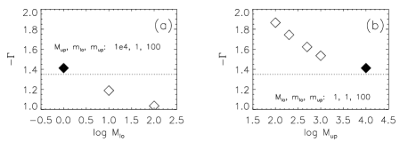
Figure 1: Dependence of logarithmic IMF slope $\Gamma$ on the lower and upper clump mass limits.

It is therefore natural to believe that the hierarchical fragmentation of molecular clouds into clumps and clumps into stars takes place self similarly according to a –2 power law mass distribution, therefore implying that the true, raw stellar IMF has this $\alpha=-2$ relation. So why is the observed Salpeter IMF slightly steeper? The answer lies in the mass range of the stars ($m_{\rm lo}$ to $m_{\rm up}$) relative to that of their parent clumps ($M_{\rm lo}$ to $M_{\rm up}$). If a cluster is generated from a single cloud, then its IMF is that for the aggregate of all stars formed out of all the clumps in this cloud. These clumps are described by a –2 power law. If $M_{\rm lo}<m_{\rm up}$, then the smallest clumps are too small to produce the highest-mass stars, thus slightly suppressing the formation of the highest-mass stars for the aggregate cluster. It turns out that the Salpeter slope results for the condition $M_{\rm lo}\sim m_{\rm lo}$ and $M_{\rm up}\gg m_{\rm up}$ (Oey 2011).

Figure 1$a$ shows the results of Monte Carlo simulations of cluster populations generated by drawing both clump and stellar masses from a power law with slope $\alpha=-2$. We assume a stellar mass range of $m_{\rm lo}=1\ \mbox{${\rm M}_{\odot}$}$ to $m_{\rm up}=100\ \mbox{${\rm M}_{\odot}$}$, and a high upper-mass limit for the clumps, $M_{\rm up}=10^{4}\ \mbox{${\rm M}_{\odot}$}$. Figure 1$a$ shows the dependence of the logarithmic IMF slope $\Gamma=\alpha+1$ as a function of lower clump mass $M_{\rm lo}$. At the highest value of $M_{\rm lo}=100\ \mbox{${\rm M}_{\odot}$}$, the mass ranges for the stars and clumps do not overlap, and essentially all stellar masses can be formed in all clumps. We therefore see that the IMF has the same value as its raw, input slope. But as $M_{\rm lo}$ decreases to values $<m_{\rm up}$, the formation of the highest-mass stars is suppressed, since they can no longer form in the smaller clumps. This steepens the aggregate IMF slope. We see that a value close to the Salpeter slope (shown by the dotted line) results for the condition $M_{\rm lo}=m_{\rm lo}$.

The models in Figure 1$b$ keep $M_{\rm lo}=1\ \mbox{${\rm M}_{\odot}$}$ fixed as $M_{\rm up}$ decreases. The black points in Figures 1$a$ and $b$ represent the same model for which the stellar mass range is 1 – 100 ${\rm M}_{\odot}$ and the clump mass range is 1 – $10^{4}\ \mbox{${\rm M}_{\odot}$}$. We see that the IMF slope continues to steepen, approaching a value near $\Gamma=-1.9$ when $M_{\rm up}=m_{\rm up}$ and $M_{\rm lo}=m_{\rm lo}$. Thus, the stellar mass range and clump mass range are exactly coincident for that model. Oey (2011) discusses the effect of additional parameters.

The Monte Carlo simulations show that the Salpeter slope corresponds to the particular condition that $M_{\rm lo}=m_{\rm lo}$ and $M_{\rm up}\gg m_{\rm up}$. The condition for $M_{\rm up}$ is reasonable, but is $M_{\rm lo}\leq m_{\rm lo}$? We note that the Salpeter slope applies only to the upper-mass tail of the IMF, and it is truncated at the lower-mass end by the observed turnover near 1 ${\rm M}_{\odot}$. This feature is generally believed to be linked to the Jeans mass, or in any case, some physics that is not scale-free. Therefore, the relevant lower clump mass is that which produces 1 ${\rm M}_{\odot}$ stars. And in fact, we do know that the power-law, clump mass function extends down to $1\ \mbox{${\rm M}_{\odot}$}$. Note that we have discussed this analysis in terms of a 100% star formation efficiency. However, the results are independent of the star formation efficiency, provided that it is constant across all clump masses. Thus, $M$ represents the clump mass capable of forming that total stellar mass, rather than the physical clump mass itself. Therefore, the relevant physical $M_{\rm lo}$ is much larger than 1 ${\rm M}_{\odot}$ for star formation effiencies $<100$%.

2 Supporting Evidence

Since we observe the clump mass function to have a power law distribution to well below the masses needed to form individual 1 ${\rm M}_{\odot}$ stars, this therefore implies that if star formation is indeed a hierarchical process, then the resulting aggregate IMF for an entire star cluster must be steeper than the raw IMF because of the suppression of the highest stellar masses in the smallest clumps. The observed Salpeter slope of $\alpha=-2.35$ cleanly implies such a steepening from a raw IMF having $\alpha=-2$, which we argued above is an eminently reasonable value to expect from first principles.

Other observations are also consistent with this model. As seen in Figure 1, our simulations show that any real scatter in the IMF should be limited between values of roughly $\Gamma=-1$ to –2. This is indeed the range seen in the observed IMF slopes, as shown by Kroupa (2002).

In addition, starbursts are sometimes suggested to have somewhat flatter IMF slopes. The Arches cluster near the Galactic center is the best-studied example, showing a slope of $\Gamma=-1$ (Espinoza et al. 2009; Kim et al. 2009). This flattening can be understood if starbursts are forming stars so intensely that the stars form faster than the cloud fragmentation timescale. Thus the starburst IMF directly reflects the raw IMF, rather than an aggregate formed out of cloud fragments. In other words, we could think of the entire starbursting cloud as a single giant, star-forming clump.

Finally, this steepening of the aggregate IMF slope relative to component sub-regions is in fact seen in the large-scale numerical simulations of Bonnell et al. (2003, 2008). As shown by Maschberger et al. (2010), the IMF slope steepens from $\alpha\sim-1.9$ to –2.2 between the subregions and the total aggregrate in the simulation totaling $10^{4}\ \mbox{${\rm M}_{\odot}$}$, in agreement with our predictions in Figure  1$a$.

3 Conclusion

We stress that a model of hierarchical star formation must lead to steepening of the aggregate IMF slope if the star-forming clumps have masses $M_{\rm lo}\ll m_{\rm up}$ (Oey 2011). We know this condition to be true empirically within star clusters. If the hierarchical process is self-similar, then this implies that the Salpeter slope $\alpha=-2.35$ results from a clump mass function having $\alpha=-2$, which is a reasonable slope to expect from first principles. This scenario is supported by both observations and theoretical simulations.

- (1) Bonnell, I. A., Bate, M. R., & Vine, S. G. 2003, MNRAS 343, 413
- (2) Bonnell, I. A., Clark, P., & Bate, M. R. 2008, MNRAs 389, 1556
- (3) Cartwright, A. & Whitworth, A. P. 2012, MNRAS 423, 1018
- (4) Elmegreen, B. G. & Efremov, Y. N. 1997, ApJ 480, 235
- (5) Espinoza, P., Selman, F. J., & Melnick, J. 2009, A&A, 501, 563
- (6) Kim, S. S., Figer, D. F., Kudritzki, R. P., & Najarro, F. 2006, ApJL, 653, L113
- (7) Kroupa, P. 2002, Science 205, 82
- (8) Maschberger, T., Clarke, C. J., Bonnell, I. A., & Kroupa, P. 2010, MNRAS, 404, 1061
- (9) Salpeter, E. E. 1955, ApJ 121, 161
- (10) Oey, M. S. 2011, ApJ 739, L46
- (11) Oey, M. S. & Clarke, C. J. 1998, AJ 115, 1543
- (12) Oey, M. S., King, N. L., & Parker, J. W. 2004, AJ 127, 1632
- (13) Zhang, Q. & Fall, S. M. 1999, ApJL 527, L81
- (14) Zinnecker, H. 1982, Annals NY Acad. Sci. 395, 226