Nucleon sea and the five-quark components

Abstract:

We generalize the approach of Brodsky et al. for the intrinsic charm quark distribution in the nucleons to the light-quark sector involving intrinsic $\bar{u},\bar{d},s$ and $\bar{s}$ sea quarks. We compare the calculations with the existing $\bar{d}-\bar{u}$, $s+\bar{s}$, and $\bar{u}+\bar{d}-s-\bar{s}$ data. The good agreement between the theory and the data is interpreted as evidence for the existence of the intrinsic light-quark sea in the nucleons. The probabilities for the $|uudu\bar{u}\rangle$, $|uudd\bar{d}\rangle$ and $|uuds\bar{s}\rangle$ Fock states are also extracted.

1 Introduction

The origin of sea quarks of the nucleons remains a subject of intense interest in hadron physics. The possible existence of a significant $uudc\bar{c}$ five-quark Fock component in the proton was proposed some time ago by Brodsky, Hoyer, Peterson, and Sakai (BHPS) [1] to explain the unexpectedly large production rates of charmed hadrons at large forward $x_{F}$ region. The intrinsic charm originating from the five-quark Fock state is to be distinguished from the “extrinsic” charm produced in the splitting of gluons into $c\bar{c}$ pairs, which is well described by QCD. The extrinsic charm has a “sea-like” characteristics with large magnitude only at the small $x$ region. In contrast, the intrinsic charm is “valence-like” with a distribution peaking at larger $x$. The presence of the intrinsic charm component can lead to a sizable charm production at the forward rapidity ($x_{F}$) region.

The CTEQ collaboration [2] has examined all relevant hard-scattering data and concluded that the data are consistent with a broad range of the intrinsic charm magnitude, ranging from null to 2-3 times larger than the estimate by the BHPS model. This suggests that more precise experimental measurements are needed for determining the magnitude of the intrinsic charm component.

In an attempt to further study the role of five-quark Fock states for intrinsic quark distributions in the nucleons, we have extended the BHPS model to the light quark sector and compared the predictions with the experimental data. The BHPS model predicts the probability for the $uudQ\bar{Q}$ five-quark Fock state to be approximately proportional to $1/m_{Q}^{2}$, where $m_{Q}$ is the mass of the quark $Q$ [1]. Therefore, the light five-quark states $uudu\bar{u}$, $uudd\bar{d}$ and $uuds\bar{s}$ are expected to have significantly larger probabilities than the $uudc\bar{c}$ state. This suggests that the light quark sector could potentially provide more clear evidence for the presence of the five-quark Fock states, allowing predictions of the BHPS model, such as the shape of the antiquark $x$ distributions originating from the five-quark configuration, to be tested.

To search for evidence of the intrinsic five-quark Fock states, it is essential to separate the contributions of the intrinsic quark and the extrinsic one. Fortunately, there exist some experimental observables which are free from the contributions of the extrinsic quarks. As discussed below, the $\bar{d}-\bar{u}$ and the $\bar{u}+\bar{d}-s-\bar{s}$ are examples of quantities independent of the contributions from extrinsic quarks. The $x$ distribution of $\bar{d}-\bar{u}$ has been measured in Drell-Yan experiments [3, 4]. A recent measurement of $s+\bar{s}$ in a semi-inclusive deep-inelastic scattering (DIS) experiment [5] also allowed the determination of the $x$ distribution of $\bar{u}+\bar{d}-s-\bar{s}$. In this paper, we compare these data with the calculations based on the intrinsic five-quark Fock states. The qualitative agreement between the data and the calculations provides evidence for the existence of the intrinsic light-quark sea in the nucleons [6]. We also show how the probabilities of various fine-quark states can be determined [7].

2 Momentum distributions of five-quark states

For a $|uudQ\bar{Q}\rangle$ proton Fock state, the probability for quark $i$ to carry a momentum fraction $x_{i}$ is given in the BHPS model [1] as

$$P(x_{1},...,x_{5})=N_{5}\delta(1-\sum_{i=1}^{5}x_{i})[m_{p}^{2}-\sum_{i=1}^{5}\frac{m_{i}^{2}}{x_{i}}]^{-2},$$ (1)

where the delta function ensures momentum conservation. $N_{5}$ is the normalization factor, and $m_{i}$ is the mass of quark $i$. In the limit of $m_{4,5}>>m_{p},m_{1,2,3}$, where $m_{p}$ is the proton mass, Eq. 1 becomes

$$P(x_{1},...,x_{5})=\tilde{N}_{5}\frac{x_{4}^{2}x_{5}^{2}}{(x_{4}+x_{5})^{2}}\delta(1-\sum_{i=1}^{5}x_{i}),$$ (2)

where $\tilde{N}_{5}=N_{5}/m_{4,5}^{4}$. Eq. 2 can be readily integrated over $x_{1}$, $x_{2}$, $x_{3}$ and $x_{4}$, and the heavy-quark $x$ distribution [1] is:

$$P(x_{5})=\frac{1}{2}\tilde{N}_{5}x_{5}^{2}[\frac{1}{3}(1-x_{5})(1+10x_{5}+x_{5}^{2})-2x_{5}(1+x_{5})\ln(1/x_{5})].$$ (3)

One can integrate Eq. 3 over $x_{5}$ and obtain the result ${\cal P}^{c\bar{c}}_{5}=\tilde{N}_{5}/3600$, where ${\cal P}^{c\bar{c}}_{5}$ is the probability for the $|uudc\bar{c}\rangle$ five-quark Fock state. An estimate of the magnitude of ${\cal P}^{c\bar{c}}_{5}$ was given by Brodsky et al. [1] as $\approx 0.01$, based on diffractive production of $\Lambda_{c}$. This value is consistent with a bag-model estimate [8].

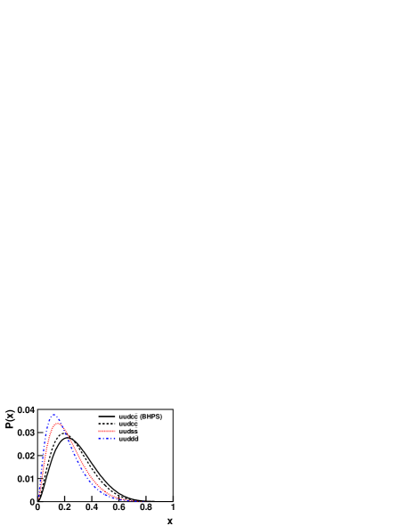
Figure 1: The $x$ distributions of the intrinsic $\bar{Q}$ in the $uudQ\bar{Q}$ configuration of the proton from the BHPS model. The solid curve is obtained using the expression in Eq. 2.3 for $\bar{c}$. The other three curves, corresponding to $\bar{c}$, $\bar{s}$, and $\bar{d}$ in the five-quark configurations, are obtained by solving Eq. 2.1 numerically. The same probability, ${\cal P}^{Q\bar{Q}}_{5}=0.01$, is used for the three different five-quark states.

The solid curve in Fig. 1 shows the $x$ distribution for the charm quark ($P(x_{5})$) using Eq. 3, assuming ${\cal P}^{c\bar{c}}_{5}=0.01$. Since this analytical expression was obtained for the limiting case of infinite charm-quark mass, it is of interest to compare this result with calculations without such an assumption. To this end, we have developed the algorithm to calculate the quark distributions using Eq. 1 with Monte-Carlo techniques. The five-quark configuration of $\{x_{1},...,x_{5}\}$ satisfying the constraint of Eq. 1 is randomly sampled. The probability distribution $P(x_{i})$ can be obtained numerically with an accumulation of sufficient statistics. We first verified that the Monte-Carlo calculations in the limit of very heavy charm quarks reproduce the analytical result for $P(x_{5})$ in Eq. 3. We then calculated $P(x_{5})$ using $m_{u}=m_{d}=0.3$ GeV, $m_{c}=1.5$ GeV, and $m_{p}=0.938$ GeV, and the result is shown as the dashed curve in Fig. 1. The similarity between the solid and dashed curves shows that the assumption adopted for deriving Eq. 3 is adequate. It is important to note that the Monte-Carlo technique allows us to calculate the quark $x$ distributions for other five-quark configurations when $Q$ is the lighter $u$, $d$, or $s$ quark, for which one could no longer assume a large mass.

As shown in Fig. 1, we have calculated the $x$ distributions of the $\bar{s}$ and $\bar{d}$ quarks in the BHPS model for the $|uuds\bar{s}\rangle$ and $|uudd\bar{d}\rangle$ configurations, respectively, using Eq. 1. The mass of the strange quark is chosen as 0.5 GeV. In order to focus on the different shapes of the $x$ distributions, the same value of ${\cal P}^{Q\bar{Q}}_{5}$ is assumed for various five-quark states. Figure 1 shows that the $x$ distributions of the intrinsic $\bar{Q}$ shift progressively to lower $x$ as the mass of the quark $Q$ decreases. The challenge is to identify proper experimental observables which allow a clear separation of the intrinsic light quark component from the extrinsic QCD component. As we discuss next, the quantities $\bar{d}(x)-\bar{u}(x)$, $s(x)+\bar{s}(x)$, and $\bar{u}(x)+\bar{d}(x)-s(x)-\bar{s}(x)$ are suitable for studying the intrinsic light-quark components of the proton.

3 Extraction of various five-quark components

To compare the experimental data with the prediction based on the intrinsic five-quark Fock state, it is necessary to separate the contributions of the intrinsic sea quark and the extrinsic one. The $\bar{d}(x)-\bar{u}(x)$ is an example of quantities which are free from the contributions of the extrinsic sea quarks, since the perturbative $g\to Q\bar{Q}$ processes will generate $u\bar{u}$ and $d\bar{d}$ pairs with equal probabilities and have no contribution to this quantity. The $\bar{d}(x)-\bar{u}(x)$ data from the Fermilab E866 Drell-Yan experiment at the $Q^{2}$ scale of 54 GeV² [4] are shown in Fig. 2.

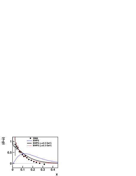
Figure 2: Comparison of the $\bar{d}(x)-\bar{u}(x)$ data with the calculations based on the BHPS model. The dashed curve corresponds to the calculation using Eq. 2.1, and the solid and dotted curves are obtained by evolving the BHPS result to $Q^{2}=54.0$ GeV² using $\mu=0.5$ GeV and $\mu=0.3$ GeV, respectively.

In the BHPS model, the $\bar{u}$ and $\bar{d}$ are predicted to have the same $x$-dependence if $m_{u}=m_{d}$. However, the probabilities of the $|uudd\bar{d}\rangle$ and $|uudu\bar{u}\rangle$ configurations, ${\cal P}^{d\bar{d}}_{5}$ and ${\cal P}^{u\bar{u}}_{5}$, are not known from the BHPS model, and remain to be determined from the experiments. Non-perturbative effects such as Pauli-blocking [9] could lead to different probabilities for the $|uudd\bar{d}\rangle$ and $|uudu\bar{u}\rangle$ configurations. Nevertheless the shape of the $\bar{d}(x)-\bar{u}(x)$ distribution shall be identical to those of $\bar{d}(x)$ and $\bar{u}(x)$ in the BHPS model. Moreover, the normalization of $\bar{d}(x)-\bar{u}(x)$ is known from the measurement of Fermilab E866 Drell-Yan experiment [4] as

$$\int^{1}_{0}(\bar{d}(x)-\bar{u}(x))dx={\cal P}^{d\bar{d}}_{5}-{\cal P}^{u\bar{u}}_{5}=0.118\pm 0.012.$$ (4)

Figure 2 shows the calculation of the $\bar{d}(x)-\bar{u}(x)$ distribution (dashed curve) from the BHPS model, together with the data. The $x$-dependence of the $\bar{d}(x)-\bar{u}(x)$ data is not in good agreement with the calculation. It is important to note that the $\bar{d}(x)-\bar{u}(x)$ data in Fig. 2 were obtained at a rather large $Q^{2}$ of 54 GeV² [4]. In contrast, the relevant scale, $\mu^{2}$, for the five-quark Fock states is expected to be much lower, around the confinement scale. This suggests that the apparent discrepancy between the data and the BHPS model calculation in Fig. 2 could be partially due to the scale dependence of $\bar{d}(x)-\bar{u}(x)$. We adopt the value of $\mu=0.5$ GeV, which was chosen by Glück, Reya, and Vogt [10] in their attempt to generate gluon and quark distributions in the so-called “dynamical approach” starting with only valence-like distributions at the initial $\mu^{2}$ scale and relying on evolution to generate the distributions at higher $Q^{2}$. We have evolved the predicted $\bar{d}(x)-\bar{u}(x)$ distribution from $Q_{0}^{2}=\mu^{2}=0.25$ GeV² to $Q^{2}=54$ GeV². Since $\bar{d}(x)-\bar{u}(x)$ is a flavor non-singlet parton distribution, its evolution from $Q_{0}$ to $Q$ only depends on the values of $\bar{d}(x)-\bar{u}(x)$ at $Q_{0}$, and is independent of any other parton distributions. The solid curve in Fig. 2 corresponds to $\bar{d}(x)-\bar{u}(x)$ from the BHPS model evolved to $Q^{2}=$ 54 GeV². Significantly improved agreement with the data is now obtained. This shows that the $Q^{2}$-evolution should be properly taken into account. It is interesting to note that an excellent fit to the data can be obtained if $\mu=0.3$ GeV is chosen (dotted curve in Fig. 2) rather than the more conventional value of $\mu=0.5$ GeV. We have also found good agreement between the HERMES $\bar{d}(x)-\bar{u}(x)$ data at $Q^{2}=2.3$ GeV² [11] with calculation using the BHPS model.

We now consider the extraction of the $|uuds\bar{s}\rangle$ five-quark component from existing data. The HERMES collaboration reported the determination of $x(s(x)+\bar{s}(x))$ over the range of $0.02<x<0.5$ at $Q^{2}=2.5$ GeV² from the measurement of charged kaon production in semi-inclusive DIS reaction [5]. The HERMES data, shown in Fig. 3, exhibits an intriguing feature. A rapid fall-off of the strange sea is observed as $x$ increases up to $x\sim 0.1$, above which the data become relatively independent of $x$. The data suggest the presence of two different components of the strange sea, one of which dominates at small $x$ $(x<0.1)$ and the other at larger $x$ $(x>0.1)$. This feature is consistent with the expectation that the strange-quark sea consists of both the intrinsic and the extrinsic components having dominant contributions at large and small $x$ regions, respectively. In Fig. 2 we compare the data with calculations using the BHPS model with $m_{s}=0.5$ GeV. The solid and dashed curves are results of the BHPS model calculations evolved to $Q^{2}=2.5$ GeV² using $\mu=0.5$ GeV and $\mu=0.3$ GeV, respectively. The normalizations are obtained by fitting only data with $x>0.1$ (solid circles in Fig. 3), following the assumption that the extrinsic sea has negligible contribution relative to the intrinsic sea in the valence region. Figure 3 shows that the fits to the data are quite adequate, allowing the extraction of the probability of the $|uuds\bar{s}\rangle$ state as

$${\cal P}^{s\bar{s}}_{5}=0.024~{}~{}(\mu=0.5~{}\rm{GeV});~{}~{}~{}{\cal P}^{s\bar{s}}_{5}=0.029~{}~{}(\mu=0.3~{}\rm{GeV}).$$ (5)

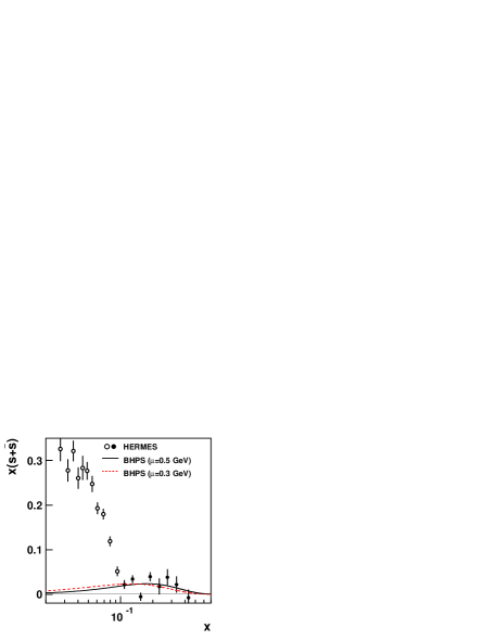
Figure 3: Comparison of the HERMES $x(s(x)+\bar{s}(x))$ data with the calculations based on the BHPS model. The solid and dashed curves are obtained by evolving the BHPS result to $Q^{2}=2.5$ GeV² using $\mu=0.5$ GeV and $\mu=0.3$ GeV, respectively. The normalizations of the calculations are adjusted to fit the data at $x>0.1$.

We consider next the quantity $\bar{u}(x)+\bar{d}(x)-s(x)-\bar{s}(x)$. Combining the HERMES data on $x(s(x)+\bar{s}(x))$ with the $x(\bar{d}(x)+\bar{u}(x))$ distributions determined by the CTEQ group (CTEQ6.6) [12], the quantity $x(\bar{u}(x)+\bar{d}(x)-s(x)-\bar{s}(x))$ can be obtained and is shown in Fig. 4. This approach for determining $x(\bar{u}(x)+\bar{d}(x)-s(x)-\bar{s}(x))$ is identical to that used by Chen, Cao, and Signal in their study of strange quark sea in the meson-cloud model [13].

An important property of $\bar{u}+\bar{d}-s-\bar{s}$ is that the contribution from the extrinsic sea vanishes, just like the case for $\bar{d}-\bar{u}$. Therefore, this quantity is only sensitive to the intrinsic sea and can be compared with the calculation of the intrinsic sea in the BHPS model. We have

$$\bar{u}(x)+\bar{d}(x)-s(x)-\bar{s}(x)=P^{u\bar{u}}(x_{\bar{u}})+P^{d\bar{d}}(x_{\bar{d}})-2P^{s\bar{s}}(x_{\bar{s}}).$$ (6)

where $P^{Q\bar{Q}}(x_{\bar{Q}})$ refers to the $x$-distribution of $\bar{Q}$ in the $|uudQ\bar{Q}\rangle$ state. We can now compare the $x(\bar{u}(x)+\bar{d}(x)-s(x)-\bar{s}(x))$ data with the calculation using the BHPS model. Since $\bar{u}+\bar{d}-s-\bar{s}$ is a flavor non-singlet quantity, we can readily evolve the BHPS prediction to $Q^{2}=2.5$ GeV² using $\mu=0.5$ GeV and the result is shown as the solid curve in Fig. 4. It is interesting to note that a better fit to the data can again be obtained with $\mu=0.3$ GeV, shown as the dashed curve in Fig. 4.

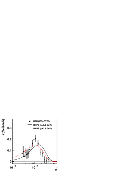
Figure 4: Comparison of the $x(\bar{d}(x)+\bar{u}(x)-s(x)-\bar{s}(x))$ data with the calculations based on the BHPS model. The values of $x(s(x)+\bar{s}(x))$ are from the HERMES experiment [5], and those of $x(\bar{d}(x)+\bar{u}(x))$ are obtained from the PDF set CTEQ6.6 [12]. The solid and dashed curves are obtained by evolving the BHPS result to $Q^{2}=2.5$ GeV² using $\mu=0.5$ GeV and $\mu=0.3$ GeV, respectively. The normalization of the calculations are adjusted to fit the data.

From the comparison between the data and the BHPS calculations shown in Figs. 2-4, we can determine the probabilities for the $|uudu\bar{u}\rangle$, $|uudd\bar{d}\rangle$, and $|uuds\bar{s}\rangle$ configurations as follows:

$${\cal P}^{u\bar{u}}_{5}=0.122;~{}~{}{\cal P}^{d\bar{d}}_{5}=0.240;~{}~{}{\cal P}^{s\bar{s}}_{5}=0.024~{}~{}~{}(\mu=0.5~{}\rm{GeV})$$ (7)

or

$${\cal P}^{u\bar{u}}_{5}=0.162;~{}~{}{\cal P}^{d\bar{d}}_{5}=0.280;~{}~{}{\cal P}^{s\bar{s}}_{5}=0.029~{}~{}~{}(\mu=0.3~{}\rm{GeV})$$ (8)

depending on the value of the initial scale $\mu$. It is remarkable that the $\bar{d}(x)-\bar{u}(x)$, the $s(x)+\bar{s}(x)$, and the $\bar{d}(x)+\bar{u}(x)-s(x)-\bar{s}(x)$ data not only allow us to check the predicted $x$-dependence of the five-quark Fock states, but also provide a determination of the probabilities for these states.

Equation 7 shows that the combined probability for proton to be in the $|uudQ\bar{Q}\rangle$ states is around 40%. It is worth noting that an earlier analysis of the $\bar{d}-\bar{u}$ data in the meson cloud model concluded that proton has $\sim$60% probability to be in the three-quark bare-nucleon state [14], in qualitative agreement with the finding of this study. A significant outcome of the present work is the extraction of the $|uuds\bar{s}\rangle$ component, which is related to the kaon-hyperon states in the meson cloud model. It is also worth noting that the $|uudQ\bar{Q}\rangle$ states have the same contribution to the proton’s magnetic moment as the $|uud\rangle$ three-quark state, since $Q$ and $\bar{Q}$ in the $|uudQ\bar{Q}\rangle$ states have no net magnetic moment. Therefore, the good description of the nucleon’s magnetic moment by the constituent quark model is preserved even with the inclusion of a sizable five-quark components.

We note that the probability for the $|uuds\bar{s}\rangle$ state is smaller than those of the $|uudu\bar{u}\rangle$ and the $|uudd\bar{d}\rangle$ states. This is consistent with the expectation that the probability for the $|uudQ\bar{Q}\rangle$ five-quark state is roughly proportional to $1/m^{2}_{Q}$ [1, 15]. One can now estimate that the probability for the intrinsic charm from the $|uudc\bar{c}\rangle$ Fock state, ${\cal P}^{c\bar{c}}_{5}$ to be roughly $0.1{\cal P}^{s\bar{s}}_{5}\sim 0.003$. This shows that the probability of intrinsic charm could be smaller than the earlier expectation [1]. Moreover, the $Q^{2}$-evolution would shift the intrinsic-charm distribution to smaller $x$, suggesting that the most promising region to search for evidence of intrinsic charm could be at the somewhat lower $x$ region $(0.1<x<0.4)$, rather than the largest $x$ region explored by previous experiments.

4 Conclusion

In conclusion, we have generalized the existing BHPS model to the light-quark sector and compared the calculation with the $\bar{d}-\bar{u}$, $s+\bar{s}$, and $\bar{u}+\bar{d}-s-\bar{s}$ data. The qualitative agreement between the data and the calculations provides strong support for the existence of the intrinsic $u$, $d$ and $s$ quark sea and the adequacy of the BHPS model. This analysis also led to the determination of the probabilities for the five-quark Fock states for the proton involving light quarks only. This result could guide future experimental searches for the intrinsic $c$ quark sea or even the intrinsic $b$ quark sea [16], which could be relevant for the production of Higgs boson at LHC energies [17]. This analysis could also be readily extended to the hyperon and meson sectors. The connections between the BHPS model, the meson-cloud model [18], the multi-quark models [19, 20], and the lattice QCD calculations [21] should also be investigated.

References

- [1] S.J. Brodsky, P. Hoyer, C. Peterson, and N. Sakai, Phys. Lett. B 93, 451 (1980); S.J. Brodsky, C. Peterson, and N. Sakai, Phys. Rev. D 23, 2745 (1981).
- [2] J. Pumplin, H. L. Lai, and W. K. Tung, Phys. Rev. D 75, 054029 (2007).
- [3] A. Baldit et al. (NA51 Collaboration), Phys. Lett. B 332, 244 (1994).
- [4] E. A. Hawker et al. (E866/NuSea Collaboration), Phys. Rev. Lett. 80, 3715 (1998); J. C. Peng et al., Phys. Rev. D 58, 092004 (1998); R.S. Towell et al., Phys. Rev. D 64, 052002 (2001).
- [5] A. Airapetian et al. (HERMES Collaboration), Phys. Lett. B 666, 446 (2008).
- [6] W. C. Chang and J. C. Peng, Phys. Rev. Lett. 80, 252002 (2011).
- [7] W. C. Chang and J. C. Peng, Phys. Lett. B 704, 197 (2011).
- [8] J. F. Donoghue and E. Golowich, Phys. Rev. D 15, 3421 (1977).
- [9] R. P. Feynman, Phys. Rev. Lett. 23, 1415 (1969).
- [10] M. Glück, E. Reya and A. Vogt, Z. Phys. C 48, 471 (1990); 53, 127 (1992); 67, 433 (1995).
- [11] A. Ackerstaff et al. (HERMES Collaboration), Phys. Rev. Lett. 81, 5519 (1998).
- [12] P. M. Nadolsky et al., Phys. Rev. D 78, 013004 (2008).
- [13] H. Chen, F. G. Cao, and A. I. Signal, J. Phys. G 37, 105006 (2010).
- [14] A. Szczurek, J. Speth, and G. T. Garvey, Nucl. Phys. A 570, 765 (1994).
- [15] M. Franz, V. Polyakov, and K. Goeke, Phys. Rev. D 62, 074024 (2000); S.J. Brodsky, J.C. Collins, S.D. Ellis, J.F. Gunion, and A. L. Mueller, Proceedings of 1984 Summer Study on the SSC, Snowmass, CO, 1984, Report No. DOE/ER/40048-21, P4.
- [16] X.G. He and B.Q. Ma, Eur. Phys. J. A 47, 152 (2011).
- [17] S.J. Brodsky, B. Kopeliovich, I. Schmidt, and J. Soffer, Phys. Rev. D 73, 113005 (2006); S. J. Brodsky, A.S. Goldhaber, B. Kopeliovich, and I. Schmidt, Nucl. Phys. B 807, 334 (2009).
- [18] J. P. Speth and A. W. Thomas, Adv. Nucl. Phys. 24, 83 (1998).
- [19] Y. Zhang, L. Shao, and B.Q. Ma, Phys. Lett. B 671, 30 (2009).
- [20] C. Bourrely, J. Soffer, and F. Buccella, Eur. Phys. J. C 41, 327 (2005).
- [21] K. F. Liu, W. C. Chang, H. Y. Chang, and J. C. Peng, arXiv:1206.4339.