Thermal vortex dynamics in thin circular ferromagnetic nanodisks

Abstract

The dynamics of gyrotropic vortex motion in a thin circular nanodisk of soft ferromagnetic material is considered. The demagnetization field is calculated using two-dimensional Green’s functions for the thin film problem and fast Fourier transforms. At zero temperature, the dynamics of the Landau-Lifshitz-Gilbert equation is simulated using fourth order Runge-Kutta integration. Pure vortex initial conditions at a desired position are obtained with a Lagrange multipliers constraint. These methods give accurate estimates of the vortex restoring force constant $k_{F}$ and gyrotropic frequency, showing that the vortex core motion is described by the Thiele equation to very high precision. At finite temperature, the second order Heun algorithm is applied to the Langevin dynamical equation with thermal noise and damping. A spontaneous gyrotropic motion takes place without the application of an external magnetic field, driven only by thermal fluctuations. The statistics of the vortex radial position and rotational velocity are described with Boltzmann distributions determined by $k_{F}$ and by a vortex gyrotropic mass $m_{G}=G^{2}/k_{F}$, respectively, where $G$ is the vortex gyrovector.

I Introduction: Vortex states in thin nanoparticles

Vortices in nanometer-sized thin magnetic particlesUsov93 have attracted a lot of attention, due to the possibilities for application in resonators or oscillators, in detectors, as objects for data storage.Guslienko+08 We consider the dynamic motion of an individual vortex in a thin circular disk (radius $R$ and height $L\ll R$) of soft ferromagnetic material such as Permalloy-79 (Py) where vortices have been commonly studied.Cowburn+99 ; Schneider+00 In disks of appropriate size, the single vortex state is very stable and of lower energy than a single-domain state.Raabe+00 Especially, we study the effective force constant $k_{F}$ responsible for the restoring force on a vortex when it is displaced from the disk center, ${\bf F}=-k_{F}{\bf X}$, where ${\bf X}$ is the vortex core position relative to the disk center. If the vortex is initially displaced from the disk center, say, by a pulsed magnetic field,Park++03 it oscillates in the gyrotropic mode,Guslienko++02 at an angular frequency $\omega_{G}=k_{F}/G$, where ${\bf G}=G\hat{z}$ is the vortex gyrovector, pointing perpendicular to the plane of the disk. The vortex gyrotropic motion has been observed, for example, by photo emission electron microscopy using x-rays.Guslienko++06 Not only in small disks but in many easy-plane magnetic models this type of vortex dynamics has been studied for its interesting gyrotropic dynamics.Volkel++91 ; Wysin+93 The gyrotropic mode is due to the translational modeWysin96 ; Ivanov+98 in a whole spectrum of internal vibrations of a magnetic vortex.WysinVolkel96

The force constant estimated analytically by Guslienko et al.Guslienko++02 using the two-vortices modelMetlov+02 gave predictions of the gyrotropic frequencies obtained in micromagnetic simulations, with reasonably good accord between the two. Here, we discuss direct numerical calculations of $k_{F}$ based on static vortex energies, by using a Lagrange multipliers technique to secure the vortex position ${\bf X}$ at a desired location,Wysin2010 and map out its potential within the disk. We apply an adapted two-dimensional (2D) micromagnetics approach for thin systems to calculate the demagnetization field. As a result, the calculations can be directly compared with the two-vortices prediction for $k_{F}$.

At the same time, we give a corresponding study of the vortex dynamics to calculate the gyrotropic frequencies. It is found that the static results for $k_{F}$ combined with the dynamics results for $\omega_{G}$ agree with the prediction of the Thiele dynamical equation,Thiele73 ; Huber82 $\omega_{G}=k_{F}/G$, to very high precision. Similar to Ref. Guslienko++02, , $k_{F}$ is found to be close to linear in the aspect ratio $L/R$ if the disks are thin but not so thin that the vortex would be destabilized. Our values for $k_{F}$ are slightly less than those in the two-vortices model, as the numerical relaxation of the vortex structure allows for more flexibility than an analytic expression.

A micromagnetics study of this systemMachado+11 for finite temperature shows evidence for a spontaneous gyrotropic vortex motion with a radius of a couple of nanometers, without the application of a magnetic field. The spontaneous gyrotropic motion occurs even if the vortex is initiated at the center of the disk in the simulations. It is clear that thermal fluctuations should lead to a random displacement of the vortex core away from the disk center, however, it is striking that the ordered gyrotropic rotation appears and even dominates over the thermal fluctuations. Here we confirm this effect, and also find that a spin wave doubletIvanov++10 (of azimuthal quantum numbers $m=\pm 1$) is excited together with the gyrotropic motion.

Having at hand the force constant $k_{F}$, we can analyze both the dynamics and the statistics of the gyrotropic motion induced by the temperature. The study of the finite temperature dynamics is carried out using a magnetic Langevin equation that includes stochastic magnetic fields together with damping. We discuss the solution via the second order Heun methodGarcia+98 ; Nowak00 applied to magnetic systems. Further, we introduce a technique for estimating the location of the vortex core accurately in the presence of fluctuations. Based on the behavior of $k_{F}$ with disk geometry, we find it possible to predict the RMS displacement of the vortex core in equilibrium. By using the collective coordinate Hamiltonian for the vortex, as derived from the Thiele equation, it is also possible to determine the probability distributions for vortex radial displacement $r=|{\bf X}|$ and rotational velocity $V=\omega_{G}r$. It is interesting to see that the velocity distribution, $f(V)$, is of the Boltzmann form for a particle with an effective mass given by $m_{G}=G^{2}/k_{F}$, which is found to depend only on the gyromagnetic ratio $\gamma$, the magnetic permeability of free space $\mu_{0}$ and the disk radius.

II Discrete model for the continuum magnet

We determine the magnetic dynamics for a continuum magnetic particle, but using a thin-film micromagnetics approach,Huang03 defining appropriate dipoles at cells of a two-dimensional grid. This is a modification of usual micromagneticsSuess06 where a 3D grid is used. The particle has a thickness $L$ along the $z$-axis, and a circular cross-section of radius $R$. For thin film magnets it is reasonable to make the assumption that the magnetization $\vec{M}({\bf r})$ does not depend on the coordinate $z$ through the thickness. This is acceptable as long as the particle is very thin. The demagnetization field tends to cause $M$ to lie within the $xy$ plane in most of the sample,Gioia97 except for the vortex core region. Even in the vortex core, however, one should not expect large variations of $M$ with $z$, due to the dominance of the ferromagnetic exchange over the dipolar interactions through short distances. In this situation for very thin magnets, this 2D approach has the obvious advantage of greater speed over 3D approaches, without sacrificing accuracy. It is somewhat like using a single layer of computation cells in 3D micromagnetics, with the cell height longer than its transverse dimensions.

The energy of the original continuum system, including exchange and magnetic field energy, can be expressed as a volume integral,

$${\cal H}=\int dV\left\{A\nabla\vec{m}\cdot\nabla\vec{m}-\mu_{0}\left[\vec{H}^{\rm ext}+\tfrac{1}{2}\vec{H}^{M}\right]\cdot\vec{M}\right\}.$$ (1)

The magnetization scaled by saturation magnetization $M_{s}$ is used to define the scaled magnetization $\vec{m}=\vec{M}/M_{s}$, that enters in the exchange term, where $A$ is the exchange stiffness (about 13 pJ/m for Permalloy). The last term is the interaction with an externally generated field, $\vec{H}^{\rm ext}$. The demagnetization energy involves the demagnetization field $\vec{H}^{M}$ that is generated by $\vec{M}$, and which is determined through a Poisson equation involving the scalar magnetic potential $\Phi_{M}$,

$$\vec{H}^{M}=-\vec{\nabla}\Phi_{M},\quad-\nabla^{2}\Phi_{M}=\rho_{M}\equiv-\vec{\nabla}\cdot\vec{M}.$$ (2)

This is solved formally in three dimensions using a convolution with the 3D Green’s function:

$$\Phi_{M}({\bf r}) = \int d^{3}{\bf r^{\prime}}~{}G_{\rm 3D}({\bf r-r^{\prime}})\rho_{M}({\bf r^{\prime}}),$$ (3)

$$G_{\rm 3D}({\bf r}) = \frac{1}{4\pi|{\bf r}|}.$$ (4)

However, this is reduced to an effective 2D Green’s operator, appropriate for thin magnetic film problems, reviewed below.

II.1 The micromagnetics model

The micromagneticsCervera99 ; Garcia03 is set up to use nanometer-scaled cells in which to define coordinates $\vec{m}_{i}$ as the averaged scaled magnetization in that cell. The system is divided into cells of size $a\times a\times L$ ($a\times a$ is the cross section in the $xy$-plane), rather than cubical cells. Each cell $i$ contains a magnetic moment of fixed magnitude $\mu=La^{2}M_{s}$, where $M_{s}$ is the saturation magnetization. The direction of the (assumed uniform) magnetization in a cell is a unit vector, $\hat{m}_{i}$, whose dynamics is to be found. The cells interact with neighboring cells via the exchange interaction, and with all other cells, due to the demagnetization field, and also with any external field.

For the square grid of cells, the exchange energy is found to be equivalent to

$${\cal H}_{\rm ex}=-2AL\sum_{(i,j)}\hat{m}_{i}\cdot\hat{m}_{j}$$ (5)

where the sum is over nearest neighbor cell pairs. The energy scale of exchange is taken as the basic energy unit. Thus it is convenient to define an effective exchange constant acting between the cells,

$$J=2AL,$$ (6)

and for the computations, all other energies will be measured in this unit. In addition, the saturation magnetization is a convenient unit for magnetic fields as well as for $\vec{M}$. So we define scaled fields,

$$\tilde{H}^{M}\equiv\frac{\vec{H}^{M}}{M_{s}},\quad\tilde{H}^{\rm ext}\equiv\frac{\vec{H}^{\rm ext}}{M_{s}}.$$ (7)

As a result of this, the magnetic field interaction energy terms are scaled here as follows. For the demagnetization,

$${\cal H}_{\rm demag}=-\frac{Ja^{2}}{2\lambda_{\rm ex}^{2}}\sum_{i}\tilde{H}_{i}^{M}\cdot\hat{m}_{i},$$ (8)

and for the energy in the external field,

$${\cal H}_{\rm ext}=-\frac{Ja^{2}}{\lambda_{\rm ex}^{2}}\sum_{i}\tilde{H}_{i}^{\rm ext}\cdot\hat{m}_{i}.$$ (9)

These depend on the definition of the exchange length,

$$\lambda_{\rm ex}=\sqrt{\frac{2A}{\mu_{0}M_{s}^{2}}},$$ (10)

that gives a measure of the competition between exchange and dipolar forces. This means that the effective 2D Hamiltonian can be written as

$${\cal H} = -J\left\{\sum_{(i,j)}\hat{m}_{i}\cdot\hat{m}_{j}\right.$$ (11)

$$\left.+\frac{a^{2}}{\lambda_{\rm ex}^{2}}\sum_{i}\left(\tilde{H}_{i}^{\rm ext}+\tfrac{1}{2}\tilde{H}_{i}^{M}\right)\cdot\hat{m}_{i}\right\}.$$

II.2 The demagnetization field $\vec{H}^{M}$ in a thin film

It is important to calculate the demagnetization field efficiently and accurately, as it plays an important role in the dynamics, and is the most computational effort. An approach for thin films, described by HuangHuang03 is used here, where we need effective Green’s functions that act in 2D on the magnetization $\vec{M}(x,y)$. This is somewhat different from that used in Refs. Wysin2010, and Wysin+12, , where the in-plane part of $\vec{H}^{M}$ was calculated by first estimating the magnetic charge density $\rho_{M}$. Here, it is preferred to calculate $\vec{H}^{M}$ directly from the field $\vec{M}$, which has less steps, and is found to result in extremely precise energy conservation in the absence of damping.

By applying an integration by parts, and throwing out a surface term outside the magnet, the solution for the magnetic potential is first written as an operation on $\vec{M}$:

$$\Phi_{M}({\bf r})=\int d^{3}{\bf r^{\prime}}~{}\vec{\nabla}^{\prime}G_{\rm 3D}({\bf r-r^{\prime}})\cdot\vec{M}({\bf r^{\prime}}).$$ (12)

One can notice that this involves the propagator for the dipole potential, that is,

$$\vec{\nabla}^{\prime}G_{\rm 3D}({\bf r-r^{\prime}})=\frac{{\bf r-r^{\prime}}}{4\pi|{\bf r-r^{\prime}}|^{3}}$$ (13)

is the function whose product with a source dipole at position ${\bf r^{\prime}}$ gives the magnetic potential at ${\bf r}$ due to that dipole.

To proceed further, it is useful to consider the contributions to the vertical ($z$) and horizontal ($xy$) components of $\vec{H}^{M}$ separately. Consider a source cell centered at $(x^{\prime},y^{\prime})$, and the vertical component of $\vec{H}^{M}$ it generates, due to $M_{z}^{\prime}\equiv M_{z}(x^{\prime},y^{\prime})$, at an observer position $(x,y)$. The usual procedure is to sum over the source point $z^{\prime}$ and average over the observer position $z$. One has the contribution from this cell, of area $dA^{\prime}=dx^{\prime}dy^{\prime}$,

$$d\Phi_{M}=\frac{dA^{\prime}M_{z}^{\prime}}{4\pi}\int_{-\delta}^{\delta}dz^{\prime}~{}\frac{(z-z^{\prime})}{[\tilde{r}^{2}+(z-z^{\prime})^{2}]^{3/2}}$$ (14)

where $\delta=L/2$ and the notation $\tilde{r}^{2}=(x-x^{\prime})^{2}+(y-y^{\prime})^{2}$ is used. The integration gives

$$d\Phi_{M}=\frac{-dA^{\prime}M_{z}^{\prime}}{4\pi}\left[\frac{1}{\sqrt{\tilde{r}^{2}+(z+\delta)^{2}}}-\frac{1}{\sqrt{\tilde{r}^{2}+(z-\delta)^{2}}}\right].$$ (15)

This would also be obtained exactly the same if starting from the magnetic surface charge density. Then, its negative gradient with respect to $z$ gives the contribution to the demagnetization field. If we also do the averaging over the observer position $z$, these two operations undo each other. The field averaged in the observer cell position is

$$\langle dH_{Mz}\rangle=-\frac{1}{L}\int_{-\delta}^{\delta}dz\frac{d}{dz}\Phi_{M}=-\left.\frac{1}{L}d\Phi_{M}\right|_{-\delta}^{+\delta}.$$ (16)

Evaluation of the limits, and then including a sum over the source point ${\bf r^{\prime}}=(x^{\prime},y^{\prime})$, shows that the field is determined by convolution with an effective Green’s function in 2D,

$$H_{Mz}({\bf r}) = \int d^{2}{\bf r^{\prime}}~{}G_{zz}({\bf r-r^{\prime}})M_{z}({\bf r^{\prime}}),$$ (17)

$$G_{zz}({\bf\tilde{r}}) = \frac{1}{2\pi L}\left(\frac{1}{\sqrt{{\tilde{r}}^{2}+L^{2}}}-\frac{1}{\tilde{r}}\right).$$ (18)

In these expressions, it is understood that the positions ${\bf r}$, ${\bf r^{\prime}}$ and the displacement between the two, ${\bf\tilde{r}}={\bf r-r^{\prime}}$, are now two-dimensional. The expression for $G_{zz}$ is divergent at zero radius. However, it is a weak divergence that can be regularized for the computation on the grid, by averaging over the cell area. For removing the divergence at $\tilde{r}=0$, averaging over a circle of area equal to the cell area $a^{2}$ replaces the value of $G_{zz}(0)$ by the longitudinal demagnetization factor $N_{z}$ for cylinder of length $L$ and radius $r_{o}=a/\sqrt{\pi}$. So we set

$$G_{zz}(0)=\langle G_{zz}\rangle_{o}=-N_{z}=-\frac{1}{L}\left(L+r_{o}-\sqrt{L^{2}+r_{o}^{2}}\right).$$ (19)

The ”o” subscript refers to averaging over the circle of radius $r_{o}$. See Ref. Wysin2010, for more details. Note that $G_{zz}$ is always negative; it correctly gives the demagnetization field opposite to the magnetization $\vec{M}$ which generated $\vec{H}^{M}$.

For the in-plane components of $\vec{H}^{M}$, a similar procedure can be followed. Due to symmetry considerations, only $M_{x}$ and $M_{y}$ can contribute. One can start by finding the magnetic potential,

$$d\Phi_{M}=\frac{dA^{\prime}}{4\pi}\int_{-\delta}^{\delta}dz^{\prime}~{}\frac{(x-x^{\prime})M_{x}^{\prime}+(y-y^{\prime})M_{y}^{\prime}}{[\tilde{r}^{2}+(z-z^{\prime})^{2}]^{3/2}}.$$ (20)

The integration over the source vertical coordinate $z^{\prime}$ gives

$$d\Phi_{M} = \frac{dA^{\prime}}{4\pi\tilde{r}^{2}}\left[(x-x^{\prime})M_{x}^{\prime}+(y-y^{\prime})M_{y}^{\prime}\right]$$ (21)

$$\times \left[\frac{z+\delta}{\sqrt{\tilde{r}^{2}+(z+\delta)^{2}}}-\frac{z-\delta}{\sqrt{\tilde{r}^{2}+(z-\delta)^{2}}}\right].$$

The averaging over the observer point $z$ can be carried out, and gives,

$$\langle d\Phi_{M}\rangle = \frac{1}{L}\int_{-\delta}^{\delta}dz~{}d\Phi_{M}(z)=\frac{\sqrt{{\bf\tilde{r}}^{2}+L^{2}}-|{\bf\tilde{r}}|}{2\pi L{\bf\tilde{r}}^{2}}$$ (22)

$$\times \left[(x-x^{\prime})M_{x}^{\prime}+(y-y^{\prime})M_{y}^{\prime}\right]dA^{\prime}.$$

Finally, the in-plane gradient leads to the in-plane demagnetization components. Including also the $z$ components, the demagnetization field averaged in the observer cell is obtained from

$$\vec{H}^{M}_{\alpha}({\bf r}) = \int d^{2}{\bf r^{\prime}}\sum_{\beta=x,y,z}G_{\alpha\beta}({\bf r-r^{\prime}})M_{\beta}({\bf r^{\prime}}).$$ (23)

The elements of the Green function needed here are found to be

$$G_{xx}({\bf\tilde{r}}) = \frac{L}{2\pi\tilde{r}^{4}}\left(\frac{\tilde{x}^{2}}{\sqrt{\tilde{r}^{2}+L^{2}}}-\frac{\tilde{y}^{2}}{\sqrt{\tilde{r}^{2}+L^{2}}+\tilde{r}}\right),$$ (24)

$$G_{xy}({\bf\tilde{r}}) = \frac{L}{2\pi\tilde{r}^{4}}\frac{2\sqrt{\tilde{r}^{2}+L^{2}}+\tilde{r}}{\sqrt{\tilde{r}^{2}+L^{2}}+\tilde{r}}\frac{\tilde{x}\tilde{y}}{\sqrt{\tilde{r}^{2}+L^{2}}}.$$ (25)

The element $G_{yy}$ is obtained from $G_{xx}$ by swapping $x$ and $y$ indices, and $G_{yx}=G_{xy}$. One can verify that these matrix elements go over to those for the far-field of a point dipole, in the limit $\tilde{r}\rightarrow\infty$.

These transverse elements of $G$ also are not defined at zero radius, because an implicit assumption in the derivation is that the observation point is outside of the source cell. There needs to be an internal demagnetization effect within a cell even for a transverse magnetization such as $M_{x}\neq 0$ or $M_{y}\neq 0$. For long thin cells with $L\gg a$, this internal transverse demagnetization factor would be approximately $N_{x}=N_{y}\approx\tfrac{1}{2}$. As a better alternative, we set $G_{xy}(0)=0$, and replace $G_{xx}(0)$ and $G_{yy}(0)$ with the transverse demagnetization factor of a cylinder with cross-sectional radius $r_{o}=a/\sqrt{\pi}$,

$$G_{xx}(0)=G_{yy}(0)=-N_{x}=\frac{1}{2L}\left(\sqrt{L^{2}+r_{o}^{2}}-r_{o}\right).$$ (26)

In this way, the internal demagnetization components of the computation cells satisfy the requirement $N_{x}+N_{y}+N_{z}=1$, while making $G_{xx}(0)$ and $G_{yy}(0)$ consistent with the regularization done for $G_{zz}(0)$.

The above results show that $\vec{H}^{M}$ is found by convolution of the 2D Green’s operator, as a matrix, with $\vec{M}$. The calculation can be made faster by using a fast Fourier transform (FFT) approach,Sasaki97 which replaces the convolution in real space with multiplication in reciprocal space. Of course, the simplest FFT approach requires a grid with a size like $2^{n}\times 2^{n}$, where $n$ is an integer. Our 2D system is a circle of radius $R=Na$ ($N$ is the size in integer grid units). For the FFT approach to work, so that the system being simulated is a single copy of the circle with no periodic interactions with the images, one can choose the smallest $n$ such that $2^{n}\geq 2N$. By making the FFT grid at least twice as large as the circle to be studied, the wrap-around problem, due to the periodicity of Fourier transforms, is avoided in the evaluation of the convolution. The FFT of the Green’s matrix, which is static, is done only once at the start of the calculation. During every time step of the integrations, however, the FFT of the magnetization field components must be carried out, for every stage at which the demagnetization field is required. Of course, the inverse FFTs to come back to $\vec{H}^{M}$ are needed as well in every stage of the time integrator.

III The dynamics and units

III.1 Zero temperature

The zero-temperature undamped dynamics of the system is determined by a torque equation, for each cell of the micromagnetics system,

$$\frac{d\vec{\mu}_{i}}{dt}=\gamma\vec{\mu}_{i}\times\vec{B}_{i}.$$ (27)

Here $\vec{B}_{i}$ is the local magnetic induction acting on the $i^{\rm th}$ cell, $\gamma$ is the electronic gyromagnetic ratio, and the dipole moment of the cell is $\vec{\mu}_{i}=La^{2}M_{s}\hat{m}_{i}$. The local magnetic induction can be defined supposing an energy $-\vec{\mu}_{i}\cdot\vec{B}_{i}$ for each dipole, with

$$\vec{B}_{i} = -\frac{\delta{\cal H}}{\delta\vec{\mu}_{i}}=-\frac{1}{\mu}\frac{\delta{\cal H}}{\delta\hat{\mu}_{i}}=\frac{J}{La^{2}M_{s}}\vec{b}_{i},$$

$$\vec{b}_{i} \equiv \sum_{j=z(i)}\hat{m}_{j}+\frac{a^{2}}{\lambda_{\rm ex}^{2}}\left(\tilde{H}_{i}^{\rm ext}+\tilde{H}_{i}^{M}\right).$$ (28)

The sum over $j$ contains only sites $z(i)$ that are nearest neighbors of site $i$. This dimensionless induction $\vec{b}_{i}$ used in the simulations is converted to real units by the following unit of magnetic induction,

$$B_{0}\equiv\frac{J}{La^{2}M_{s}}=\frac{2A}{a^{2}M_{s}}=\frac{\lambda_{\rm ex}^{2}}{a^{2}}\,\mu_{0}M_{s}.$$ (29)

For computations, the dynamics is written in terms of the dimensionless fields, also scaling the time appropriately:

$$\frac{d\hat{m}_{i}}{d\tau}=\hat{m}_{i}\times\vec{b}_{i},\quad\tau=\gamma B_{0}t.$$ (30)

This means that the unit of time in the simulations is $t_{0}=(\gamma B_{0})^{-1}$. For Permalloy with $A=13$ pJ/m, $M_{s}=860$ kA/m, one has $\lambda_{\rm ex}\approx 5.3$ nm. In our simulations we put the transverse edge of the cells as $a=2.0$ nm. Then using the gyromagnetic ratio, $\gamma=e/m_{e}\approx 1.76\times 10^{11}$ T^-1 s^-1, the computation units are based on $\mu_{0}M_{s}=1.08$ T and $B_{0}\approx 7.59$ T. This large value for $B_{0}$ is the scale of the local magnetic induction due to the exchange interaction between the cells. The time unit is then $t_{0}\approx 0.75$ ps; a frequency unit is $f_{0}=\gamma B_{0}=1.336$ THz. We may display frequency results, however, in units of $\tfrac{\mu_{0}}{4\pi}\gamma M_{s}\approx$ 15.1 GHz for Permalloy, as this expression is equivalent to $\gamma M_{s}$ in CGS units. For the disk sizes used here, typical periods of the vortex gyrotropic motion are around $\tau_{G}\sim 4000$, which then corresponds to dimensionless frequency $\nu=1/\tau_{G}\sim 2.5\times 10^{-4}$, and hence, physical frequency $f=\nu f_{0}\sim 0.3$ GHz.

In some cases we also need to include Landau-Gilbert damping, with some dimensionless strength $\alpha$. Then this is included into the dynamics with the usual modification,

$$\frac{d\hat{m}_{i}}{d\tau}=\hat{m}_{i}\times\vec{b}_{i}-\alpha\hat{m}_{i}\times\left(\hat{m}_{i}\times\vec{b}_{i}\right).$$ (31)

The zero temperature dynamics was integrated numerically for this equation, using a standard fourth-order Runge-Kutta (RK4) scheme. Typically, a time step of $\Delta\tau=0.04$ was found sufficient to insure the correct energy conserving dynamics (when $\alpha=0$) and result in total energy conserved to better than 12 digits of precision over $5.0\times 10^{5}$ time steps in a system with as many as 4000 cells. To get this high precision, however, it is necessary to always evaluate the full demagnetization field at all four intermediate stages of the individual Runge-Kutta time steps.

III.2 Finite temperature: Langevin dynamics

For non-zero temperature, the dynamics is investigated here using a Langevin approach. This requires including both a damping term and a stochastic torque in the dynamics; together they represent the interaction with a heat bath. The size of the stochastic torques is related to the temperature and the damping constant, such that the system reaches thermal equilibrium.

It is reasonable to think of the dynamics depending on stochastic magnetic inductions $\vec{b}_{s}$, in addition to the deterministic fields $\vec{b}_{i}$ from the Hamiltonian dynamics. For the discussion here, suppose we consider the dynamics of one computation cell, and suppress the $i$ index. The dynamical equation for that cell’s $\hat{m}$, including both the deterministic and random fields, is

$$\frac{d{\hat{m}}}{d\tau}=\hat{m}\times\left(\vec{b}+\vec{b}_{s}\right)-\alpha\hat{m}\times\left[\hat{m}\times\left(\vec{b}+\vec{b}_{s}\right)\right].$$ (32)

The first term is the free motion and the second term is the damping. Alternatively, the dynamics can be viewed as that due to the superposition of the deterministic effects (due to $\vec{b}$) and stochastic effects (due to $\vec{b}_{s}$).

For a given temperature $T$, the stochastic fields establish thermal equilibrium, provided the time correlations satisfy the fluctuation-dissipation (FD) theorem,

$$\langle b_{s}^{\lambda}(\tau)\,b_{s}^{\lambda^{\prime}}(\tau^{\prime})\rangle=2\alpha\,{\cal T}\,\delta_{\lambda\lambda^{\prime}}\,\delta(\tau-\tau^{\prime}).$$ (33)

$\delta_{\lambda\lambda^{\prime}}$ is the Kronecker delta and the indices $\lambda,\lambda^{\prime}$ refer to any of the Cartesian coordinates; $\delta(\tau-\tau^{\prime})$ is a Dirac delta function. The dimensionless temperature ${\cal T}$ is the thermal energy scaled by the energy unit $J$,

$${\cal T}\equiv\frac{kT}{J}=\frac{kT}{2AL},$$ (34)

where $k$ is Boltzmann’s constant. The fluctuation-dissipation theorem expresses how the power in the thermal fluctuations is carried in the random magnetic fields. In terms of the physical units, the relation is

$$\gamma\mu\langle B_{s}^{\lambda}(t)B_{s}^{\lambda^{\prime}}(t^{\prime})\rangle=2\alpha\,kT\,\delta_{\lambda\lambda^{\prime}}\,\delta(t-t^{\prime}).$$ (35)

where $\mu=La^{2}M_{s}$ is the magnetic dipole moment per computation cell.

III.3 Time evolution with second order Heun (H2) method

The Langevin equation (32) is a first-order differential equation that is linear in multiplicative noise. If $y=y(\tau)$ represents the full state of the system (a vector of dimension $3N$, where $N$ is the number of cells), then the dynamics follows an equation of the form

$$\frac{dy}{d\tau}=f[\tau,y(\tau)]+f_{s}[\tau,y(\tau)]\cdot{b}_{s}(\tau).$$ (36)

The vector function $f$ is the deterministic time derivative and the vector function $f_{s}$ determines the stochastic dynamics; $b_{s}$ represents the whole stochastic field of the system. An efficient method for integrating this type of equation forward in time is the second order Heun (H2) method.Garcia+98 ; Nowak00 That is in the family of predictor-corrector schemes and is rather stable. It involves an Euler step as the predictor stage, and a corrector stage that is equivalent to the trapezoid rule. Some details of the method are summarized here, to indicate how the stochastic fields are included, and to show why it is used rather than the fourth order Runge-Kutta method (the latter seems difficult to adapt to the stochastic fields).

We use the notation $y_{n}\equiv y(\tau_{n})$ to show the values at times $\tau_{n}=n\Delta\tau$, according to the choice of some integration time step $\Delta\tau$. Integrating Eq. (36) over one time step gives the Euler predictor estimate for $y(\tau_{n}+\Delta\tau)$:

$$\tilde{y}_{n+1}=y_{n}+f(\tau_{n},y_{n})\Delta\tau+f_{s}(\tau_{n},y_{n})\cdot(\sigma_{s}w_{n}).$$ (37)

The last factor, $\sigma_{s}w_{n}$, is introduced to represent the time-integral of the stochastic magnetic inductions. $\sigma_{s}$ is a variance and $w_{n}$ represents a vector of $3N$ random numbers, one for each Cartesian component at each site of the grid. Consider, say, the result of integrating the equation of motion for just one component for one site:

$$\int_{\tau_{n}}^{\tau_{n}+\Delta\tau}d\tau~{}b_{s}^{x}(\tau)\longrightarrow\sigma_{s}w_{n}^{x}.$$ (38)

The physical variance $\sigma_{s}$ needed for this to work correctly, must be determined by the FD theorem. For this individual component at one site, the squared variance is

$$\sigma_{s}^{2} = \left\langle\left(\int_{\tau_{n}}^{\tau_{n}+\Delta\tau}d\tau~{}b_{s}^{x}(\tau)\right)^{2}\right\rangle$$ (39)

$$= \int_{\tau_{n}}^{\tau_{n}+\Delta\tau}d\tau\int_{\tau_{n}}^{\tau_{n}+\Delta\tau}d\tau^{\prime}~{}\left\langle b_{s}^{x}(\tau)b_{s}^{x}(\tau^{\prime})\right\rangle.$$

Now applying the FD theorem to this gives the required variance of the random fields, that depends on the time step being used:

$$\sigma_{s}=\sqrt{2\alpha{\cal T}\,\Delta\tau}.$$ (40)

This means that individual stochastic field components $b_{s}^{\lambda}(\tau)$, integrated over one time step, are replaced by random numbers of zero mean with variance $\sigma_{s}$, as used above.

For the corrector stage, the points $y_{n}$ and $\tilde{y}_{n+1}$ are used to get better estimates of the slope of the solution. Then their average is used in the trapezoid corrector stage:

$$y_{n+1} = y_{n}+\frac{1}{2}\left[f(\tau_{n},y_{n})+f(\tau_{n+1},\tilde{y}_{n+1})\right]\Delta\tau$$

$$+ \frac{1}{2}\left[f_{s}(\tau_{n},y_{n})+f_{s}(\tau_{n+1},\tilde{y}_{n+1})\right]\cdot(\sigma_{s}w_{n}).$$

The error is of order ${\cal O}((\Delta\tau)^{3})$, hence it is a second order scheme. Note that the same vector of $3N$ random numbers $w_{n}$ used in the predictor stage are re-used in the corrector stage, because it is the evolution over the same time interval.

In the coding for computations, one does not use the explicit form of the functions $f$ and $f_{s}$. Rather, at each cell, first one can calculate the deterministic effective field $\vec{b}_{i}$ based on the present state of the system. Its effect in the dynamics will be actually proportional to its product with the time step, i.e., it gives a contribution $\Delta\hat{m}_{i}\propto\vec{b}_{i}\Delta\tau$. Of course, the stochastic change in this same site will be proportional to the stochastic effective field, which is some $\sigma_{s}\vec{w}_{i}$ for that site, where $\vec{w}_{i}=(w_{i}^{x},w_{i}^{y},w_{i}^{z})$. So the total change at this site is linearly determined by a combination,

$$\Delta\hat{m}_{i}\propto\vec{g}_{i},\quad\vec{g}_{i}\equiv\vec{b}_{i}\Delta\tau+\sigma_{s}\vec{w}_{i}.$$ (42)

An effective field combination $\vec{g}_{i}$ acts in this way both during the predictor and the corrector stages. In either stage, a dynamic change in a site is given by a simple relation,

$$\Delta\hat{m}_{i}=\hat{m}_{i}\times\left[\vec{g}_{i}-\alpha(\hat{m}_{i}\times\vec{g}_{i})\right].$$ (43)

Of course, the predictor stage uses the last configuration of the whole system to determine all the $\vec{b}_{i}$, while the corrector finds the needed $\vec{b}_{i}$ based on the predicted positions. And, the corrector actually does the average of $\Delta\hat{m}_{i}$ from the Euler stage and the second estimate from the corrector stage. The same random numbers $w_{n}$ used in the predictor stage are used again in the corrector, for a chosen time step.

The integration requires a long sequence of quasi-random numbers $w_{n}$. It is important that the simulation time does not surpass the period of the random numbers. We used the generator mzran13 due to Marsaglia and Zaman, mzran94 implemented in the C-language for long integers. This generator is very simple and fast and has a period of about $2^{125}$, and is based on a combination of two separate generators with periods of $2^{32}$ and $2^{95}$.

IV Vortex state properties and zero-temperature dynamics

The dynamics at zero temperature, calculated with RK4, was used to check basic vortex dynamic properties such as the stability and gyrotropic mode frequency. We also used the Langevin dynamics calculated with second order Heun method to include finite temperature to see the primary thermal effects for some specific vortex initial configurations. For some of these studies, it is extremely beneficial to produce a well-formed initial vortex state in some desired location without the presence of spin waves.

An initial vortex state is prepared first in a planar configuration of positive vorticity $q=+1$, namely, in-plane magnetization angle $\phi=\tan^{-1}m_{y}/m_{x}$ given by

$$\phi(x,y)=q\tan^{-1}\frac{x-x_{0}}{y-y_{0}}.$$ (44)

(The negative vorticity state $q=-1$ is destabilized by the demagnetization field, so there is no reason to consider it.) This is the profile of a vortex centered at position $(x_{0},y_{0})$. The out-of-plane component here is $m_{z}=0$, however, the stable vortex state has a nonzero out-of-plane component close to $m_{z}=\pm 1$ at the vortex core (polarization $p=\pm 1$). This stable vortex state was reached by the local spin alignment procedureWysin96 for a vortex at the constrained position $(x_{0},y_{0})$, described in Ref. Wysin2010, . Briefly, that is a procedure where each $\hat{m}_{i}$ is aligned along its local induction $\vec{b}_{i}$, and the process is iterated until convergence. The constraint is applied as extra fictitious fields included with the Lagrange multiplier technique, that force the desired vortex starting position. This procedure helps to remove any spin waves that would otherwise be generated starting from any arbitrary initial state. This state would be a perfect static state if generated in the center of the disk. When generated off-center, the dynamics associated with its motion still is able to produce some spin waves. A cleaner vortex motion can be generated if there is a weak damping applied ($\alpha=0.02$) over some initial time interval ($\tau\approx 1000$). After that, the system can be let to evolve in energy-conserving dynamics, if needed.

This relaxed vortex state develops either positive or negative out-of-plane component, including some small randomness in the initial state before the relaxation. If $m_{z}\approx+1$ ($-1$) in the vortex core region, the vortex has positive (negative) polarization and a positive (negative) gyrovector $G=G_{z}$, defined from

$${\bf G}=2\pi Q\frac{m_{0}}{\gamma}\,\hat{z},\quad Q\equiv qp.$$ (45)

$\gamma$ is the electron gyromagnetic ratio and $m_{0}=\mu/a^{2}=LM_{s}$ is the magnetic dipole moment per unit area. The integer $Q=\pm 1$ defines the quantized topological charge that determines the two allowed discrete values of the gyrovector. To a good degree of precision, the vortex states studied here obey a dynamics for the vortex velocity ${\bf V}$ described by a Thiele equation,Thiele73 ; Huber82 ignoring any intrinsic vortex massWysin96 or damping effects,

$${\bf F}+{\bf G}\times{\bf V}=0.$$ (46)

This equation comes from an analysis of the Hamiltonian dynamics of a magnetic system,Wysin+91 ; Volkel++91 in which the vortex excitation profile preserves its shape but moves with some collective coordinate center position ${\bf X}(t)$, with ${\bf V}(t)=\dot{\bf X}(t)$. The force ${\bf F}$ is the gradient of the potential experienced by the vortex. The force points towards the nanodisk center, and can be approximated by some harmonic potential with force constant $k_{F}$, for a vortex at distance $r$ from the center,

$${\bf F}=-k_{F}r\,\hat{r}.$$ (47)

Hence, the presence of the gyrovector leads to the well-known gyrotropic (or uniform circular) motion. Solving for the vortex velocity results in

$${\bf V}=\frac{\hat{z}\times{\bf F}}{G}=-\frac{\gamma k_{F}r}{2\pi QLM_{s}}\hat{\phi}.$$ (48)

$G$ includes the sign of the gyrovector (vector ${\bf G}$ points perpendicular to the plane of the disk, and it has only a $z$ component). Thus, the vortices generated with positive (negative) gyrovector move clockwise (counterclockwise) in the $xy$ plane. Furthermore, the angular frequency of this gyrotropic motion is given by a related equation,

$$\omega_{G}=\frac{V}{r}=-\frac{k_{F}}{G}=-\frac{\gamma k_{F}}{2\pi QLM_{s}}.$$ (49)

The force constant has been estimated theoretically from the rigid vortex approximationGuslienko++01 and from the two-vortex model.Guslienko++02 Below, we determine $k_{F}$ numerically from relaxed vortex statesWysin2010 (a flexible vortex). The frequency in Eq. (49) applies to the stable vortex states. If the disk is too thin, the vortex could be unstable; this produces an outward force ${\bf F}$, and results in the gyrotropic motion in the “wrong” direction. Thus it is easy to identify whether a vortex is stable or unstable from a short integration of its dynamics.

In the time and frequency units applied in the simulations, the dimensionless gyrotropic frequency $\Omega_{G}$ is obtained from

$$\Omega_{G}=\omega_{G}t_{0}=\frac{\omega_{G}}{\gamma B_{0}}=-\frac{k_{F}a^{2}}{4\pi LAQ}.$$ (50)

The negative sign shows that vortices with a negative gyrovector ($Q=-1$) have a counterclockwise rotational motion; the opposite sense holds for positive gyrovector. The force constant $k_{F}$ increases with thickness $L$ but decreases with disk radius $R$. Therefore, in the simulation time units, the gyrotropic frequency could depend primarily on their ratio, $L/R$.

For detection of the vortex motion, one method is to measure the spatially averaged magnetization,

$$\langle\vec{m}\rangle=\frac{1}{N}\sum_{i}\vec{m}_{i}.$$ (51)

This is a useful measure of vortex gyrotropic motion, especially for experiments, where it may not be possible to observe the rapidly changing instantaneous vortex core position. However, $\langle\vec{m}\rangle$ can show rotational oscillations even when no vortex is present. Thus, we need instead a measure of the vortex core position based on the location of the vorticity charge center.

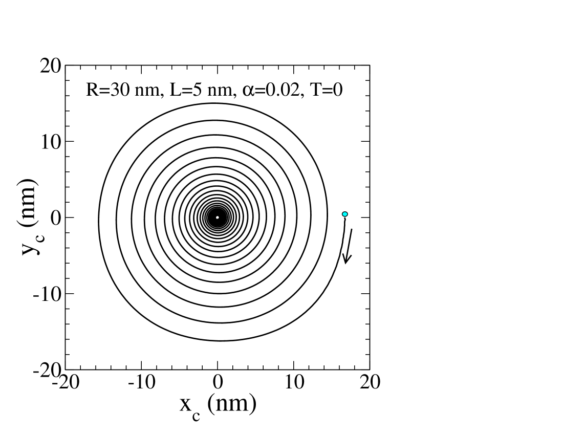
Figure 1: Vortex motion with damping, at zero temperature. This is clockwise motion for a vortex with positive ($+\hat{z}$) gyrovector, starting from the dot on the $x$-axis. The vortex performs gyrotropic motion of decreasing radius and increasing frequency as it moves towards the disk center, ${\bf r}=(0,0)$.

The vorticity center position ${\bf r}_{v}$ is the point around which the in-plane magnetization components give a divergent curl. That is, a continuum magnetization field of a vortex located at position ${\bf r}_{v}$, with in-plane angle $\phi({\bf r})$, would be expected to have the curl,

$$\vec{\nabla}\times\vec{\nabla}\phi({\bf r})=2\pi\hat{z}\delta({\bf r-r}_{v}).$$ (52)

When used on the discrete grid of cells, the vorticity center falls between the four nearest neighbor grid cells that have a net $2\pi$ circulation in $\phi$. However, this discretely defined position always jumps in increments of the cell size $a$, hence, it cannot be used directly. Instead, we use an average position weighted by the squared $m_{i}^{z}$ components, of only those cells near the vorticity center:

$${\bf r}_{c}=\frac{\sum_{|{\bf r}_{i}-{\bf r}_{v}|<4\lambda_{\rm ex}}(m_{i}^{z})^{2}\,{\bf r}_{i}}{\sum_{|{\bf r}_{i}-{\bf r}_{v}|<4\lambda_{\rm ex}}(m_{i}^{z})^{2}}.$$ (53)

The ${\bf r}_{i}$ are the cell positions and the sum is restricted to those cells within four exchange lengths of the vorticity center. The center of the nanodisk is the origin, $(x,y)=(0,0)$. Including this cutoff in the sums helps to reduce the contributions from other oscillations in the system (i.e., spin waves) that are not directly associated with the vortex position. By weighting with $(m_{i}^{z})^{2}$, the position ${\bf r}_{c}$ is able to change smoothly as the vortex moves, especially at $T=0$, in contrast to the discrete vorticity center ${\bf r}_{v}$. It is a reasonable estimate of the mean location of out-of-plane magnetization energy of the vortex, i.e., close to the vortex core position. The $m_{z}$-weighted position ${\bf r}_{c}$ and the vorticity center ${\bf r}_{v}$ are usually within one lattice constant. This measure is supplemented by observing the actual magnetization field when there is any doubt about the presence or stability of the vortex.

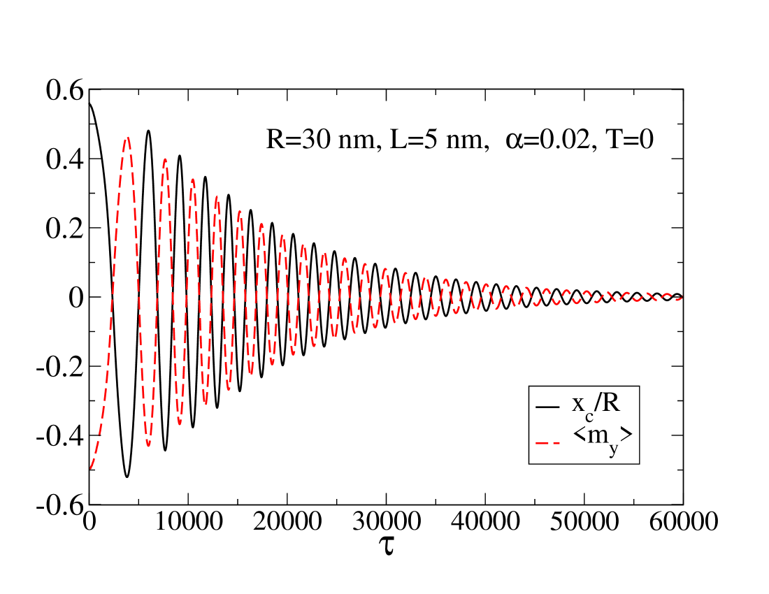
Figure 2: (Color online) For the vortex motion in Figure 1, the phase relationship between perpendicular components of position and in-plane magnetization.

IV.1 Gyrotropic frequencies in circular disks

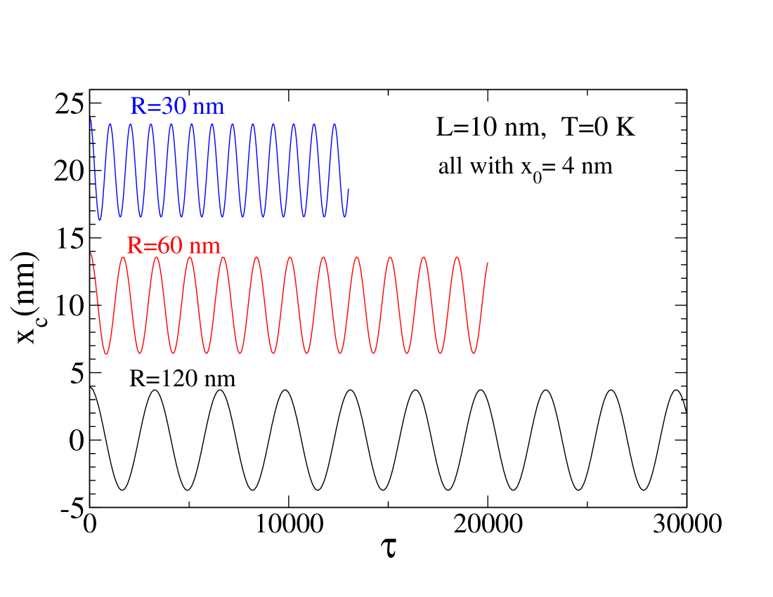
Figure 3: (Color online) Typical motions of the vortex core coordinate $x_{c}(\tau)$ at zero temperature, for circular disks of thickness $L=10$ nm with different radii (shifted vertically from $x_{c}=0$ for clarity). The damping $\alpha=0.02$ was turned off at time $\tau=1000$. Periods were calculated from the energy-conserving motion after $\tau>1000$. The motion of $y_{c}(\tau)$ is similar but shifted a quarter of a period.

Calculations were carried out for circular disks of thickness 5.0 nm, 10 nm and 20 nm ($L=2.5a,5a,10a$, all with $a=2.0$ nm) for radii 30 nm, 60 nm, 90 nm and 120 nm. The stability of the vortex state is easily checked for a given geometry, by starting from a relaxed vortex at some radius near half the radius of the disk. Including a weak damping $\alpha=0.02$, it is necessary only to run a short simulation of the dynamics and observe whether the vortex moves in the direction given by the Thiele equation,Thiele73 Eq. (48).

For example, with $R=30$ nm, $L=5.0$ nm, a vortex was initially relaxed at a position $(x_{0},y_{0})=(16,0)$ nm, and then the dynamics was started, including damping $\alpha=0.02$ in the RK4 method. In this case the vortex is very stable and spirals into the center of the disk, see Figures 1 and 2. The instantaneous vortex displacement on one axis, scaled by disk radius, takes approximately the same magnitude as the perpendicular in-plane component of $\langle\hat{m}\rangle$, such as $x_{c}/R$ and $\langle m_{y}\rangle$ in Figure 2. Another feature is that the period of rotation becomes less as the vortex moves inward. The first few periods are $\Delta\tau=6000,3140,2580,$ but the later revolutions have an average period $\tau_{G}\approx 2020$ (1.51 ns, frequency $f_{G}=1/\tau_{G}=0.661$ GHz for Py).

Other similar dynamics calculations were done at various disk sizes, but turning off the damping $\alpha=0.02$ after $\tau=1000$, see Figure 3. This initial damped motion is used to remove spin waves that might be generated when the vortex is initially released, after being relaxed at a desired starting position. Once the damping is turned off, the dynamics is energy conserving. Because we are later interested in small movements near the disk center, the initial position was taken as $(x_{0},y_{0})=(2a,0)$, using a lattice constant $a=2.0$ nm. These simulations result in very smooth circular motion of the vortex center ${\bf r}_{c}$ (Fig. 3), from which very precise estimates of the gyrotropic period $\tau_{G}$ were determined by following the motion for typically five to ten periods. The resulting frequencies $f_{G}$, in units of $\tfrac{\mu_{0}}{4\pi}\gamma M_{s}$, are shown versus aspect ratio $L/R$ in Figure 4. The scale is also given there for the parameters of Permalloy, for which $\tfrac{\mu_{0}}{4\pi}\gamma M_{s}\approx 15.1$ GHz. One can note the obvious feature, that the gyrotropic frequency goes to zero at some minimum thickness needed for vortex stability.

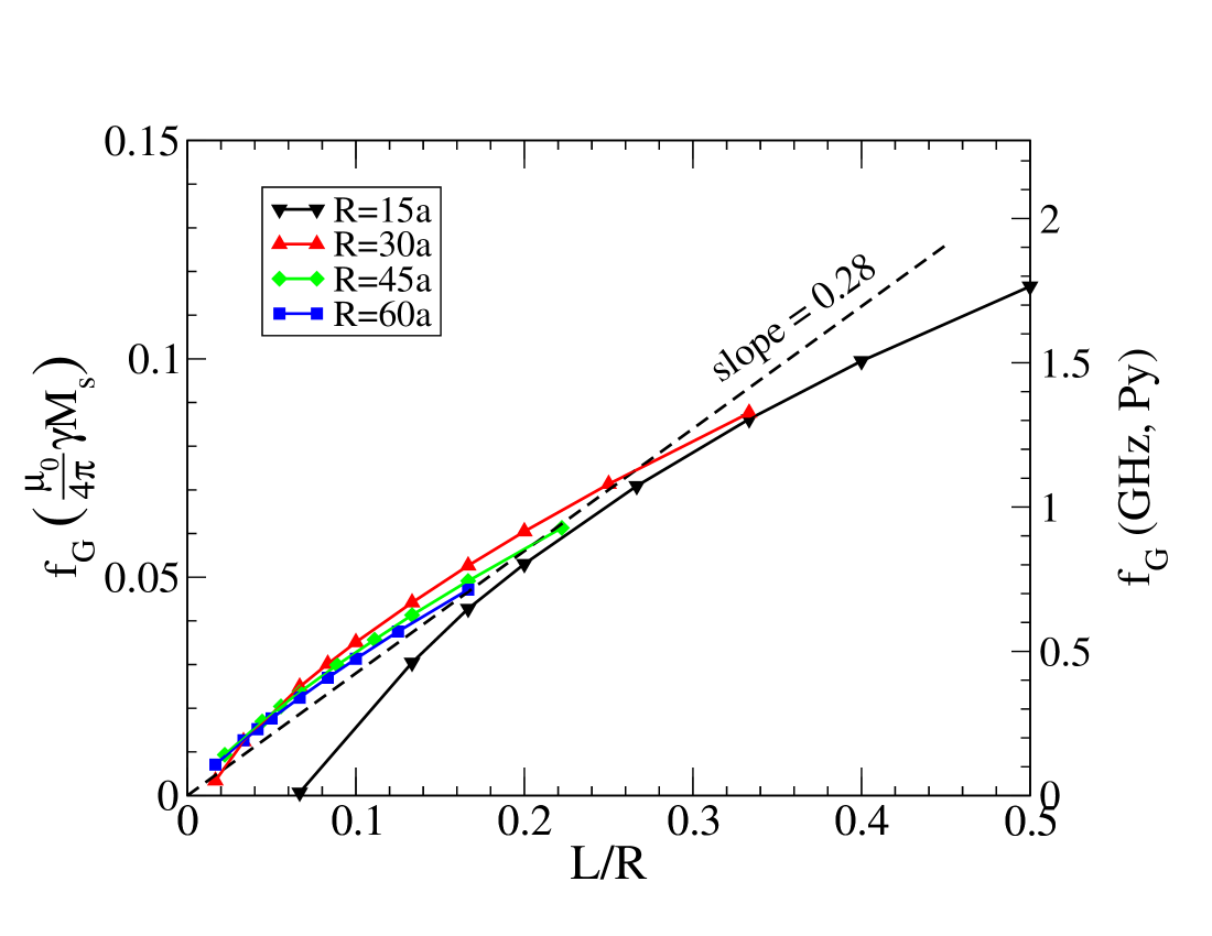
Figure 4: (Color online) Zero-temperature vortex gyrotropic frequency $f_{G}$ for various disk radii $R$, versus aspect ratio $L/R$. [For Permalloy, $\tfrac{\mu_{0}}{4\pi}\gamma M_{s}\approx 15.1$ GHz]. The computation cell size is $a=2.0$ nm. The vortex state is unstable below a minimum disk thickness, as expected due to the diminished restoring forces from the reduced edge area. The dashed line shows the result [Eq. (59)] from using the linear approximation in Eq. (55) for $k_{F}$.

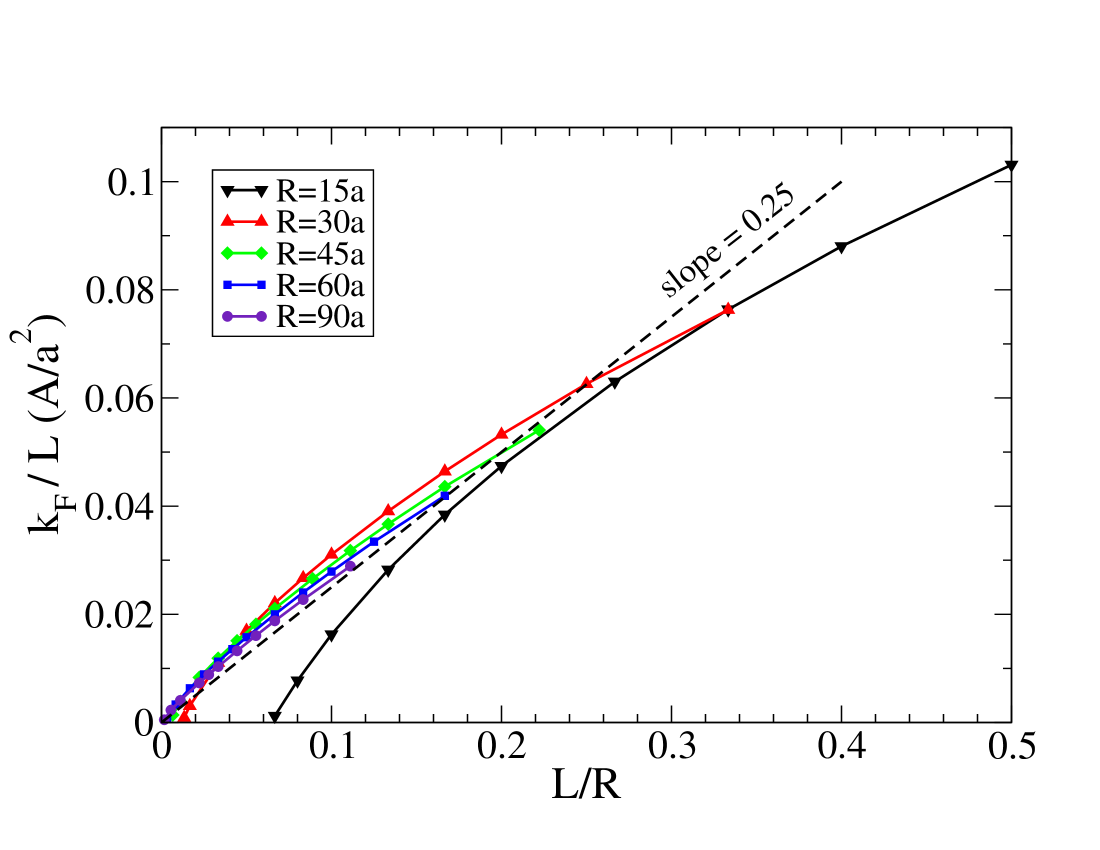
Figure 5: (Color online) Vortex force constant $k_{F}$ scaled by disk thickness, versus disk aspect ratio. These were obtained by assuming a parabolic potential for vortex motion within the disk. The dashed line indicates that the slope of this relationship is close to $1/4$ for some range of parameters, Eq. (55), for disks of adequate thickness. Cell edge is $a=2.0$ nm.

IV.2 Relation to force constant $k_{F}$

The vortex restoring force constants $k_{F}$ were estimated based only on static energy considerations. We compared the total system energy with the displaced vortex, $U(x)$, taking $x=2a$, with the energy for the vortex at the disk center, $U(0)$. It is known that the vortex potential is close to parabolic, as long as the vortex displacement is small compared to the disk radius.Wysin2010 The force constant is then estimated simply by solving

$$U(x)=U(0)+\frac{1}{2}k_{F}\,x^{2}.$$ (54)

The energies applied in this equation are those obtained after the vortex is relaxed by the Lagrange-constrained method. These calculations are relatively fast because there is no need to run the dynamics. The raw force constants were obtained for a wide variety of disk sizes. Generally, we find that $k_{F}$ increases faster than linearly with disk thickness $L$ and decreases with disk radius $R$.

It is expected that the force constant should scale somewhat with the aspect ratio, $L/R$. Further, the Thiele equation suggests that the ratio $k_{F}/L$ is most relevant in determining $\omega_{G}$ [see Eq. (49)]. Therefore, we show $k_{F}/L$ versus $L/R$ in Figure 5, which presents a relationship somewhat close to linear, with a slope near $1/4$. Thus we can write as a rough approximation (far enough from the critical disk thickness for vortex stability),

$$k_{F}\approx\frac{1}{4}\frac{L^{2}}{R}\frac{A}{a^{2}}=\frac{\lambda_{\rm ex}^{2}}{8a^{2}}\mu_{0}M_{s}^{2}\frac{L^{2}}{R}=0.878\mu_{0}M_{s}^{2}\frac{L^{2}}{R}.$$ (55)

The last form, obtained by applying the definition of exchange length, is preferred because the vortex restoring force ultimately is due to the demagnetization fields generated by $M_{s}$.

One can check whether these force constants are consistent with the gyrotropic frequencies found in the dynamics. If the Thiele equation applies to this motion, then the gyrotropic frequencies must be linearly proportional to $k_{F}/L$, [Equations (49) and (50)]. Therefore we have plotted the dimensionless frequency $\Omega_{G}$ versus $k_{F}/L$ in Figure 6. For the wide variety of disk sizes studied, all points in this plot fall on a single line of unit slope, exactly consistent with the Thiele equation. This shows that the calculations of the dynamics over fairly long times (many periods) are completely consistent with the force constants found only from static energy considerations. It further implies that we can safely use static energy calculations to predict dynamic properties. This is based on the assumption of an isotropic parabolic potential in which the vortex moves. There may be some limitation to this idea, however, only because the potential will deviate from parabolic for larger displacements from the disk center.

These results are consistent with the two-vortices model applied by Guslienko et al.Guslienko++02 With the boundary parameter $\xi=2/3$ and the initial susceptibility at small aspect ratio being $\chi(0)^{-1}\approx 9.98L/R$, their result (converted to SI units by factor $\tfrac{\mu_{0}}{4\pi}$) is approximately

$$k_{F}=\pi L\frac{\mu_{0}}{4\pi}M_{s}^{2}\xi^{2}\chi(0)^{-1}\approx 1.109\mu_{0}M_{s}^{2}\frac{L^{2}}{R}.$$ (56)

Our results have a somewhat weaker potential, which is to be expected because the numerical simulations allow for a wider range of possible deformations of the vortex structure than is possible in an analytic approximation. In addition, our numerical results include the destabilization of the vortex at sufficiently small $L/R$, hence, it is impossible to fit any straight line for $k_{F}/L$ vs. $L/R$ down to arbitrarily small aspect ratio, see Figure 5.

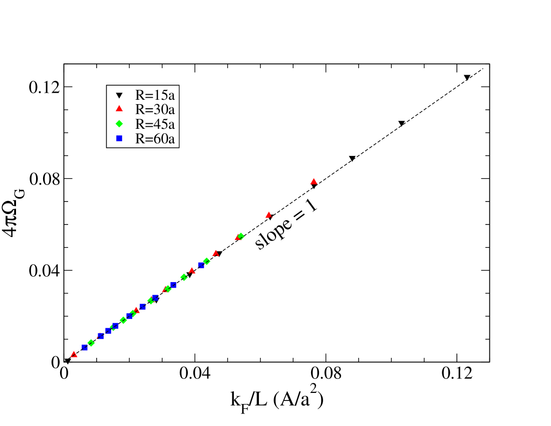
Figure 6: (Color online) The dimensionless gyrotropic frequencies (found from dynamics) versus force constant scaled by disk thickness. The dashed line of unit slope is Eq. (50). This verifies the dynamics of the Thiele equation, and shows the complete consistency between the static energetics and the dynamics. Cell edge is $a=2.0$ nm.

We showed above that the gyrotropic frequencies $\nu_{G}$ are exactly linearly proportional to $k_{F}/L$, hence, this implies that the frequencies also scale close to linearly with $L/R$. Combining our fit of $k_{F}$ with relation (50) then shows that roughly, the dimensionless angular frequency magnitude is

$$\Omega_{G}\approx\frac{1}{16\pi}\frac{L}{R}\approx 0.0199\frac{L}{R}.$$ (57)

In physical units, this is

$$\omega_{G}=\gamma B_{0}\Omega_{G}\approx 0.140\,\gamma\mu_{0}M_{s}\frac{L}{R}.$$ (58)

Then the frequency comes out

$$f_{G}=\frac{\omega_{G}}{2\pi}\approx 0.280\left(\frac{\mu_{0}}{4\pi}\gamma M_{s}\right)\frac{L}{R}.$$ (59)

The dashed line in Figure 4 shows Eq. (59) compared with data from various disk sizes. These frequencies are smaller than those in the rigid vortex model,Guslienko++01 and only slightly smaller than those for the two-vortices model.Guslienko++02 However, this result fits quite well with the experimental data presented in Ref. Guslienko++06, by also using the higher value for the gyromagnetic ratio, $\gamma=1.85\times 10^{11}$ s^-1 T^-1, in conjunction with saturation magnetization still at the value $M_{s}=860$ kA/m. The calculation here can be considered as that for a more flexible vortex. The magnetization at the edge of the disk adjusts itself to try to follow the boundary. The magnetization can also adjust itself, to a lesser extent, in the vortex core region. These effects lead to lower force constants and therefore lower gyrotropic frequencies.

These results show that the adapted 2D methods applied here give reliable results, consistent with experiment and with the two-vortices analytic calculation of the gyrotropic frequencies. We note that the smaller value of cell constant used here ($a=2.0$ nm) is important for the simulation to correctly describe the magnetization dynamics in the vortex core. Of course, this then imposes a limitation on the system size that can be studied.

These results confirm the basic dynamic properties, that the vortex resonance frequency $\omega_{G}$ diminishes with increasing dot radius, and increases with increasing dot thickness. A wider dot has a weaker spring constant $k_{F}$ in its potential, $U(r)=U(0)+\tfrac{1}{2}k_{F}r^{2}$, leading to the reduction of its resonance frequency. Similarly, in a thicker dot, the greater area at the edge produces a larger restoring force, leading to a higher resonance frequency.

V Thermal effects in vortex dynamics in circular disks

In the following part, the effects of thermal fluctuations on the vortex dynamics are considered. We consider two basic situations left to evolve in time via Langevin dynamics: (1) A vortex started off-center, and (2) a vortex started at the minimum energy position, the center of the disk. In the latter case, the question is whether thermal fluctuations alone are sufficient to initiate gyrotropic motion. If so, we can also study its frequency and range of motion. In all simulations we used cell size $a=2.0$ nm and damping parameter $\alpha=0.02$ .

V.1 Vortex initially off-center

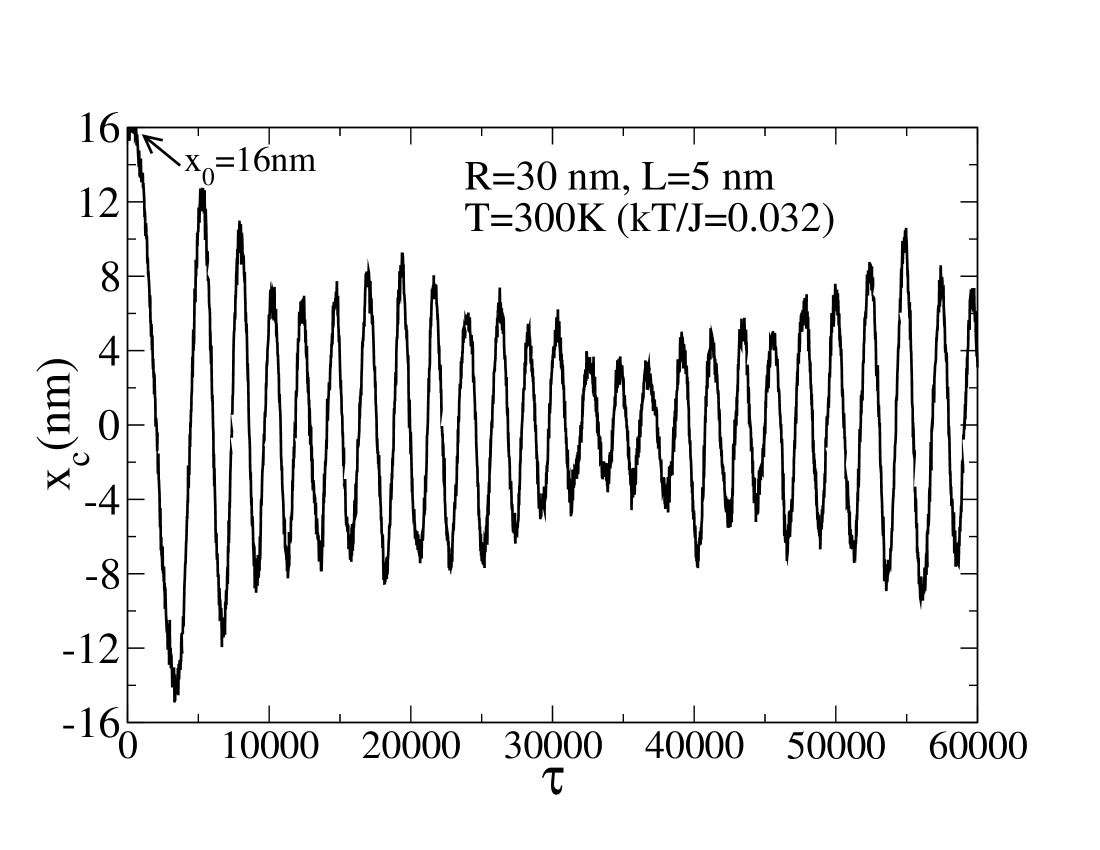
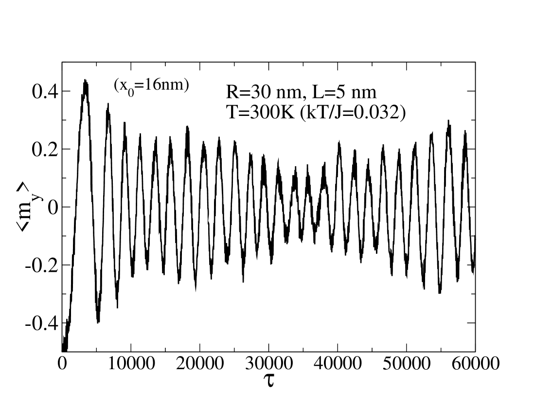
Figure 7: Vortex motion in Py at room temperature (300 K), starting from an initial displacement of 16 nm from the disk center. The $y$-component of average magnetization in the disk is correlated to the $x$-component of the vortex position.

For the same system used above [$R=30$ nm, $L=5.0$ nm], the same initial condition was used, with vortex at $(x_{0},y_{0})=(16,0)$ nm, but a finite temperature corresponding to Permalloy at 300 K was considered. The dynamics was solved now by the H2 scheme. The scaled temperature depends on the thickness $L$ of the disk and the exchange stiffness $A$ of the material. The energy unit here is $J=2AL=130$ zJ, while 300 K corresponds to $kT=4.14$ zJ, so the scaled temperature is ${\cal T}=kT/J=0.032$. The $x$-component of the vortex position versus time is shown in Figure 7. In this case, the vortex still spirals towards the center of the disk, however, thermal fluctuations remain present in the motion even at time $\tau=60000$ ($\approx 90$ ns), 25 revolutions later. The range of the motion there remains close to $\pm 6$ nm. The time dependence of $\langle m_{y}\rangle$ (most closely related to $x_{c}$) is also shown in Figure 7; it also shows an effect persisting at the 25% level out to $\tau=60000$. Note that at zero temperature, the time-scale for relaxation (Figure 2) was on the order of $\tau\sim 20000$. This shows that thermal forces apparently are able to maintain the gyrotropic motion to very long times. The average period of the motion is $\tau_{G}\approx 2278$ (1.705 ns, frequency $f=1/\tau_{G}=0.586$ GHz for Py), showing that the temperature also softened the potential experienced by the vortex.

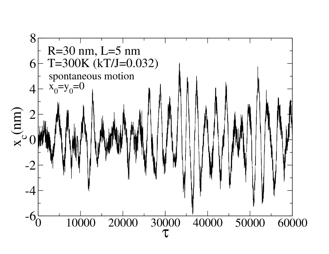
Figure 8: Spontaneous gyrotropic vortex motion in Py due to thermal fluctuations at 300 K, starting from a vortex at the center of the disk.

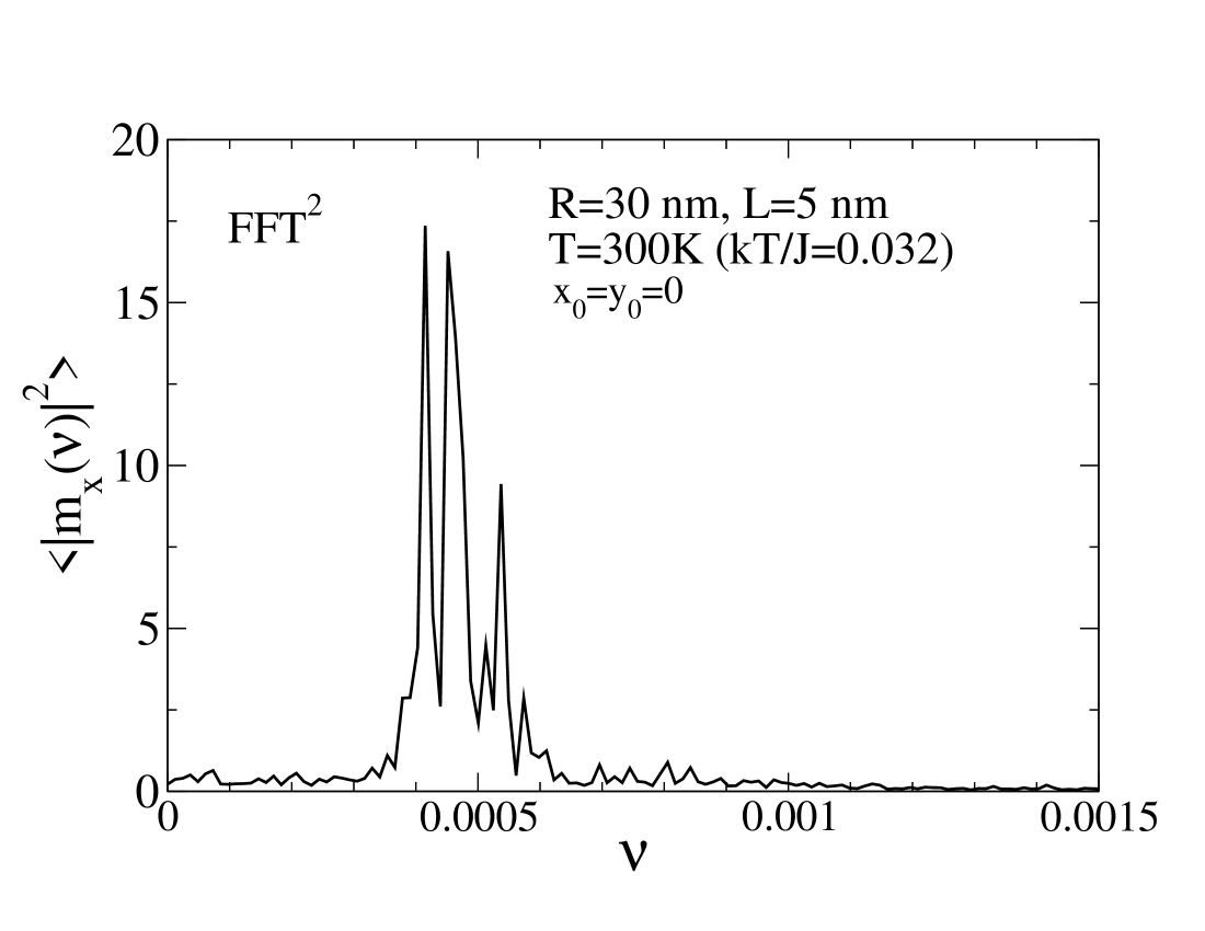
Figure 9: Thermal power spectrum of the in-plane magnetization fluctuations due to spontaneous gyrotropic vortex motion in Py at 300 K, for the motion in Figure 8.

V.2 Vortex initially at disk center

The same system is used [$R=30$ nm, $L=5.0$ nm], but this time the vortex was initiated at the center of the disk, $(x_{0},y_{0})=(0,0)$. At zero temperature, such an initial state is static. Instead, the dynamics corresponding to Py at 300 K was considered (scaled temperature ${\cal T}=0.032$). Any thermal fluctuations can move the vortex core off-center, and if that happens, gyrotropic motion can initiate spontaneously. This indeed happens, as can be seen in the vortex core position ${\bf r}_{c}(\tau)$ plotted in Figure 8. It needs to be stressed that these vortex motions of the order of $\pm 4$ nm, and magnetization fluctuations on the order of $\pm 15$%, occur without the application of any external magnetic field. The motion is sufficiently coherent that it can be followed for dozens of rotations. The gyrotropic motion was followed out to twice the time shown in the plots. An average over 24 rotations results in a period $\tau_{G}=2250$, corresponding to 1.68 ns or a frequency $f=0.594$ GHz. To verify this, we also show the power spectrum of the in-plane magnetization oscillations in Figure 9. This was obtained by taking time FFTs of $\langle m_{x}(\tau)\rangle$ of length 256 points at different starting times in the data out to $\tau=120000$ and averaging their absolute squares. The middle peak in Figure 9 falls at dimensionless frequency $\nu\approx 4.52\times 10^{-4}$, corresponding to physical frequency $f=\nu/t_{0}=0.600$ GHz, consistent with the estimate from counting oscillations. There is some structure in the FFT, possibly the beating between three different primary frequencies, that causes the amplitude of the oscillations to wax and wane.

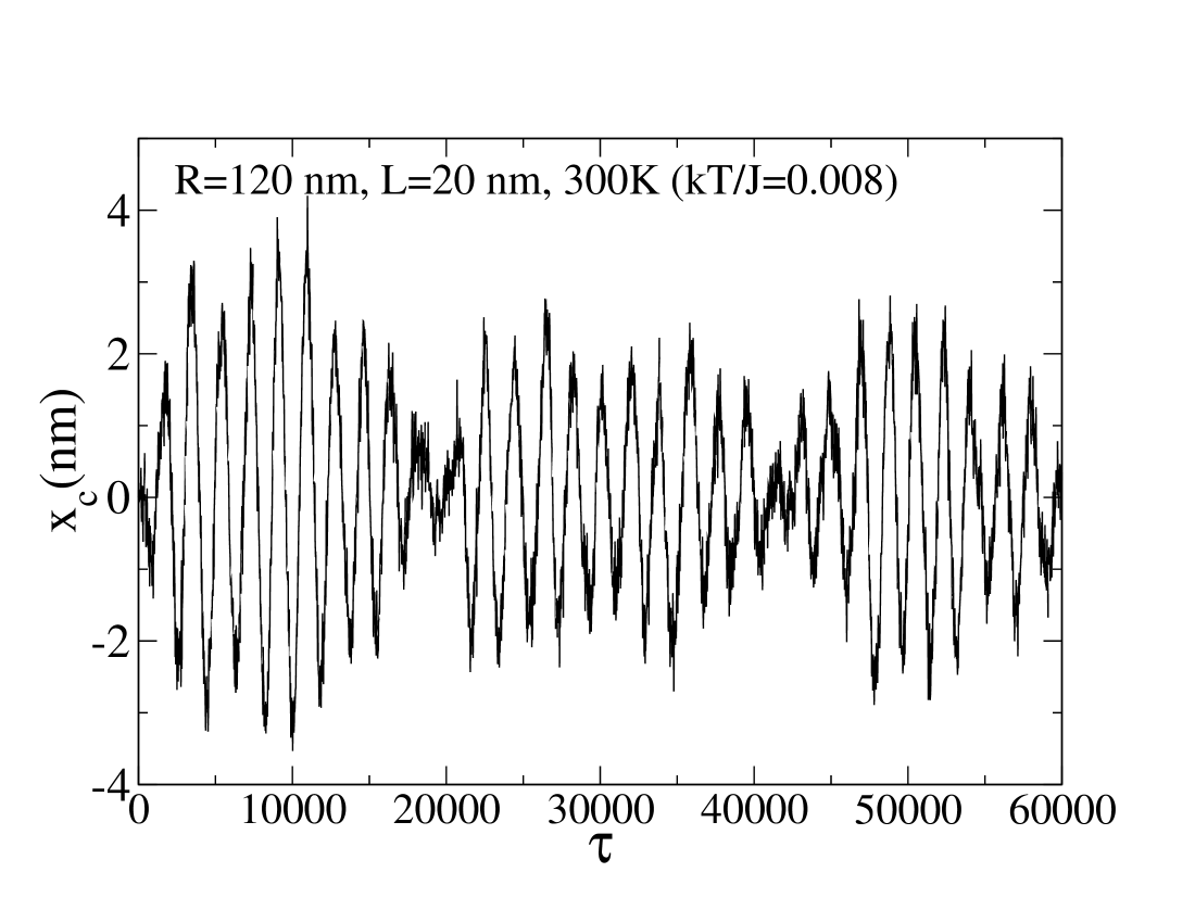
Figure 10: Spontaneous gyrotropic vortex motion, due to thermal fluctuations, in a 20 nm thick Py disk at 300 K, with the vortex starting at the center of the disk. The natural periodic motion executes 32 revolutions in this time sequence, with period $\tau_{G}\approx 1870$.

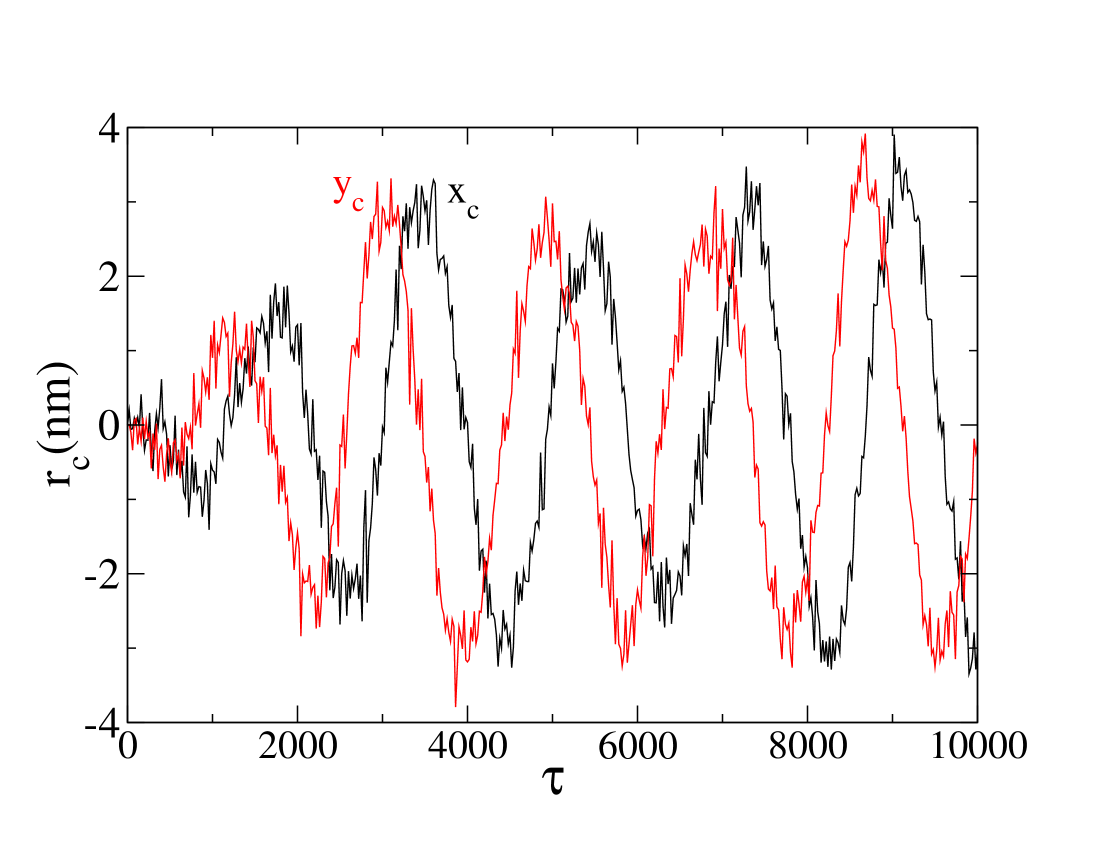
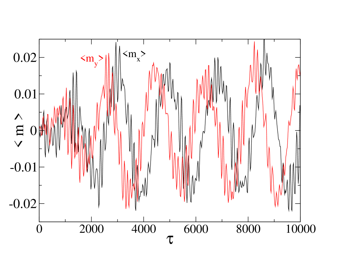
Figure 11: (Color online) For the spontaneous gyrotropic vortex motion in Figure 10, [$R=120$ nm, $L=20$ nm Py disk at 300 K], details of the motion at earlier times. The vortex started at the center of the disk. There is a high-frequency spin wave oscillation apparent in the magnetization dynamics, excited together with the gyrotropic motion.

The spontaneous gyrotropic vortex motion takes place for a wide range of system sizes that were tested. Another example is given for a larger system [$R=120$ nm, $L=20$ nm] in Figure 10, where the vortex core displacement is displayed. An interesting feature is apparent. The gyrotropic motion loses its phase coherence at times, leading randomly to brief intervals of dramatically changed amplitude. This is only one example; in other time sequences for other system sizes, this behavior is particularly intermittent and random. For the same simulation, Figure 11 also shows both components of vortex core position and both components of the average in-plane magnetization, zoomed in to show details at earlier times. Here one can see the quarter-period phase difference between $x$ and $y$ components for the vortex position as well as for the magnetization. In addition, the magnetization exhibits a high-frequency oscillation with a period of about $\Delta\tau\approx 125$ on top of the gyrotropic oscillations. This can be expected to be spin wave excitations that are excited thermally together with the vortex gyrotropic motion.

To confirm the identity of these spin wave oscillations, we also show in Figure 12 the power spectrum in net magnetization component $m_{x}$, from a longer simulation out to time $\tau=2.5\times 10^{5}$ . The vertical scale has been zoomed in to bring out the appearance of a doublet with frequencies of 9.3 GHz and 11.4 GHz, for Permalloy parameters, while the gyrotropic frequency is only 0.71 GHz. A spin wave doublet with azimuthal quantum numbers $m=\pm 1$ (wavefunction varying as $\psi\sim e^{im\phi}$ around the disk center) has been discussed in Ref. Ivanov++10, . The doublet is predicted to have a splittingGuslienko+2008 of $\Delta f=f_{2}-f_{1}=3.5f_{G}$ and an averaged frequencyZaspel+05 of $\bar{f}=1.8\left(\frac{\mu_{0}}{4\pi}\gamma M_{s}\right)\sqrt{\frac{L}{R}}$. For the situation here, these formulas predict $\Delta f=2.5$ GHz and $\bar{f}=11.1$ GHz, while the observed doublet has $\Delta f=2.1$ GHz and $\bar{f}=10.3$ GHz. Although slightly softer, these are of the right orders of magnitude and are consistent with the the theoretical prediction for this doublet. This lowest doublet relates to the presence of spin waves propagating azimuthally around the disk, in the presence of the vortex. The splitting can be attributed to the breaking of symmetry for the two directions of propagation, due to the presence of the out-of-plane magnetization at the vortex core. Based on these results and results at other disk sizes, we then note that the primary deviation from a smooth gyrotropic motion is due to the thermal excitation of this doublet on top of the vortex magnetization.

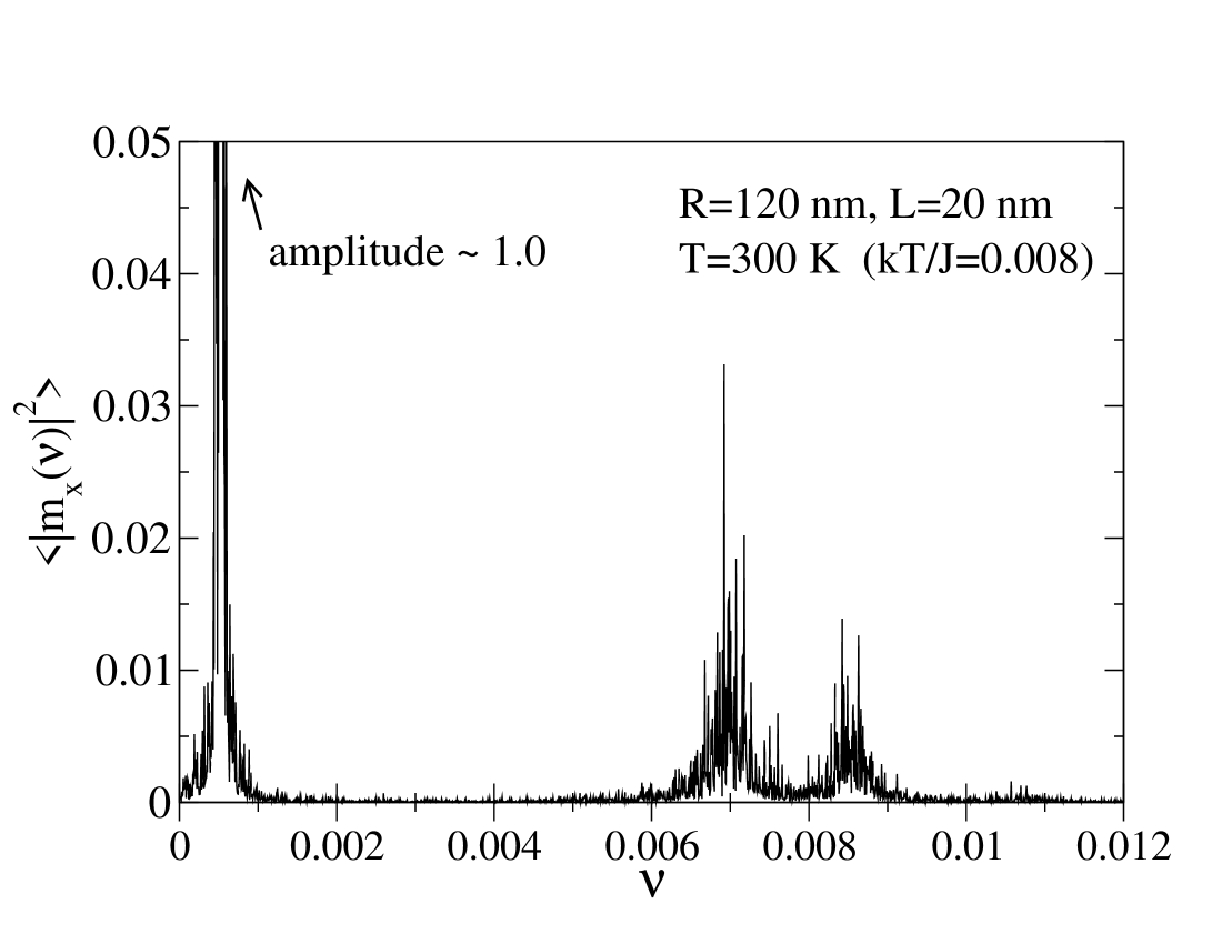
Figure 12: (Color online) The thermally averaged power spectrum in one component of the magnetization (squared FFT) for the vortex motion in Figure 10. The low frequency gyrotropic mode dominates strongly over a much weaker doublet at high frequency. For Permalloy parameters ($f={\rm 1336GHz}\times\nu$), the gyrotropic frequency is $f_{G}=0.71$ GHz while the components of the doublet lie at $f_{1}=9.3$ GHz and $f_{2}=11.4$ GHz.

V.3 Analysis of thermal vortex motion in circular nanodisks

The spontaneous vortex motion at 300 K takes place without the application of any externally generated magnetic field. Only the thermal energy is responsible for the motion. Indeed, both the frequency and amplitude of this spontaneous gyrotropic motion is determined directly by the temperature. Here we give some analysis and suggest where this motion might be most easily observed experimentally.

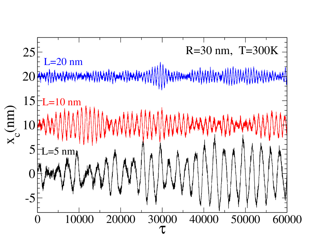
Figure 13: (Color online) Typical spontaneous fluctuations of the vortex core $x$-coordinate for 30 nm radius Py disks with various thicknesses, at 300 K. The vortex was initiated at the disk center. Curves are shifted vertically from $x_{c}=0$ for clarity.

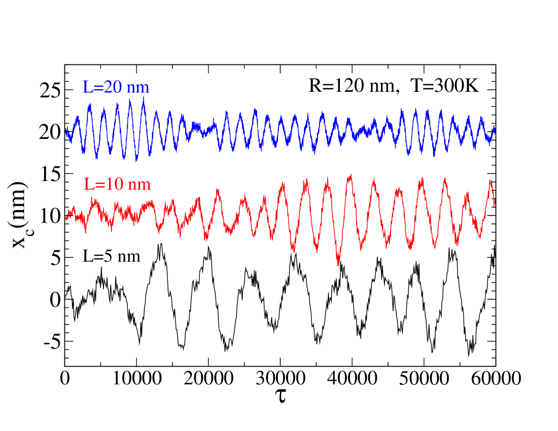
Figure 14: (Color online) Typical spontaneous fluctuations of the vortex core $x$-coordinate for 120 nm radius Py disks with various thicknesses, at 300 K. The vortex was initiated at the disk center. Curves are shifted vertically from $x_{c}=0$ for clarity.

For some smaller disks with $R=30$ nm, and for some larger disks, with $R=120$ nm, Figures 13 and 14 exhibit the typical time dependence of the vortex coordinate $x_{c}(\tau)$, for Permalloy systems at 300 K. The vortex was initially relaxed at the center of the disk ($x=y=0$). As seen for the systems studied above, the gyrotropic motion is spontaneous, and furthermore, takes place at a lower frequency for thinner disks. In addition, there is a dependence of the amplitude of the motion on the disk thickness. The amplitude is observed to be larger for thinner disks. Also it is apparent that generally the amplitude is larger for the larger radius disks. This is somewhat difficult to analyze precisely, due to the limited time sequences that can be obtained during a reasonable computation time. However, from knowledge of the force constants $k_{F}$ and their dependence on the disk geometry, the RMS range of the vortex core motion can be predicted.

The statistical mechanics of the vortex core position ${\bf X}=(X(t),Y(t))$ and velocity ${\bf V}=\dot{\bf X}$ can be obtained from the effective Hamiltonian associated with the Thiele equation. The Thiele equation is mathematically equivalent to the equation of motion for a massless charge $e$ in a uniform magnetic field ${\bf B}$, with $e{\bf B}=-{\bf G}$, and also affected by some other force ${\bf F}$. We can start from a Lagrangian that leads to the Thiele equation, using the symmetric gauge for the effective vector potential, and including a circularly symmetric parabolic potential (harmonic approximation),

$$L({\bf X},\dot{\bf X})=-\tfrac{1}{2}G(X\dot{Y}-Y\dot{X})-\tfrac{1}{2}k_{F}(X^{2}+Y^{2}).$$ (60)

The first term on the RHS is equivalent to $e{\bf V}\cdot{\bf A}$, with vector potential ${\bf A}=\tfrac{1}{2}{\bf B}\times{\bf X}$ in a magnetic problem; there is no usual kinetic energy term like $\tfrac{1}{2}m{\bf V}^{2}$, because the intrinsic mass is considered zero here. Only the $z$-component of the gyrovector is present, $G\equiv G_{z}=2\pi pqm_{0}\gamma^{-1}$. Then the components of the Thiele equation are recovered from the Euler-Lagrange variations,

$$\frac{\partial L}{\partial X}-\frac{d}{dt}\frac{\partial L}{\partial\dot{X}}=-k_{F}X-G\dot{Y}=0,$$ (61)

$$\frac{\partial L}{\partial Y}-\frac{d}{dt}\frac{\partial L}{\partial\dot{Y}}=-k_{F}Y+G\dot{X}=0.$$ (62)

The Lagrangian is written equivalently as

$$L({\bf X},{\bf V})=-\tfrac{1}{2}({\bf G}\times{\bf X})\cdot{\bf V}-\tfrac{1}{2}k_{F}{\bf X}^{2}.$$ (63)

This leads to the canonical momentum,

$${\bf P}=\frac{\partial L}{\partial\bf V}=-\tfrac{1}{2}{\bf G}\times{\bf X}=(\tfrac{G}{2}Y,-\tfrac{G}{2}X).$$ (64)

This allows the transformation to the collective coordinate Hamiltonian, $H({\bf X},{\bf P})$. Following the usual prescription, we have

$$H({\bf X},{\bf P})={\bf P}\cdot\dot{\bf X}-L=\frac{1}{2}k_{F}{\bf X}^{2}=\frac{1}{2}k_{F}\left(X^{2}+Y^{2}\right).$$ (65)

Note that the derivation of the Hamiltonian does not depend on the choice of the gauge for the gyrovector (i.e., for its effective magnetic field). In Ref. Ivanov+2010 , it is shown that the Landau gauge leads to the same result for $H$, but where $P=GY$ is found to be the momentum conjugate to $X$.

Technically this is all that is needed to analyze the statistics of the vortex position. By being purely potential energy, however, this Hamiltonian needs careful treatment. Its variation via the Hamiltonian equations of motion does not lead back to the correct dynamics, i.e., it does not give the Thiele equation. One can see that the difficulty is due to the fact that the position and canonical momentum coordinates are redundant, since $P_{x}=\tfrac{1}{2}GY$ and $P_{y}=-\tfrac{1}{2}GX$. Even so, all of these should be considered linearly independent mechanical coordinates, and all should appear in $H$ to give the correct dynamics (gyrotropic motion does not conserve ${\bf X}$ nor ${\bf P}$, so both should appear in $H$). For that to work out, $H$ must be expressed so that there are both potential and kinetic energy terms. (A similar care is needed even in the Landau gauge, where $GY$ must be identified by and replaced as the momentum $P$ conjugate to $X$.) We can split out half of the potential energy and redefine it in terms of ${\bf P}^{2}$ as a kinetic energy,

$$H({\bf X},{\bf P})=\tfrac{1}{4}k_{F}{\bf X}^{2}+\tfrac{1}{4}k_{F}\left(\frac{2\bf P}{G}\right)^{2}.$$ (66)

One can easily demonstrate that the correct dynamic equations result only by allocating exactly half of the energy as kinetic energy and half as potential energy. This then leads to the Hamilton dynamic equations for oscillations along the two perpendicular axes. For example, along $x$ there is

$$\dot{X}=\frac{\partial H}{\partial P_{x}}=\frac{2k_{F}P_{x}}{G^{2}},$$ (67)

$$\dot{P}_{x}=-\frac{\partial H}{\partial X}=-\tfrac{1}{2}k_{F}X.$$ (68)

These give a second order equation for simple harmonic motion (SHO),

$$\ddot{X}=-\frac{k_{F}^{2}}{G^{2}}X.$$ (69)

The other variations with respect to $Y$ and $P_{y}$ lead to the same dynamics for $Y$. However, note that the Thiele equation is recovered from these dynamics only by including the connection (64) that defines the canonical momentum in terms of the position.

It is clear that the Hamiltonian (66) is the same as that for a two-dimensional simple harmonic oscillator with coordinate ${\bf X}$ and momentum ${\bf P}$. For that oscillator, the effective spring constant is $k_{\rm SHO}=\tfrac{1}{2}k_{F}$, and the corresponding effective mass is $m_{\rm SHO}=\frac{G^{2}}{2k_{F}}$. It is interesting to see that these lead back to the natural frequency of gyrotropic motion [or see Eq. (69)],

$$\omega_{G}=\omega_{\rm SHO}=\sqrt{\frac{k_{\rm SHO}}{m_{\rm SHO}}}=\frac{k_{F}}{G}.$$ (70)

Of course, as $G$ is proportional to the disk thickness via the factor $m_{0}=LM_{s}$, and $k_{F}$ depends on both $R$ and $L$, then this contains the various geometrical effects, especially those associated with the vortex force constant.

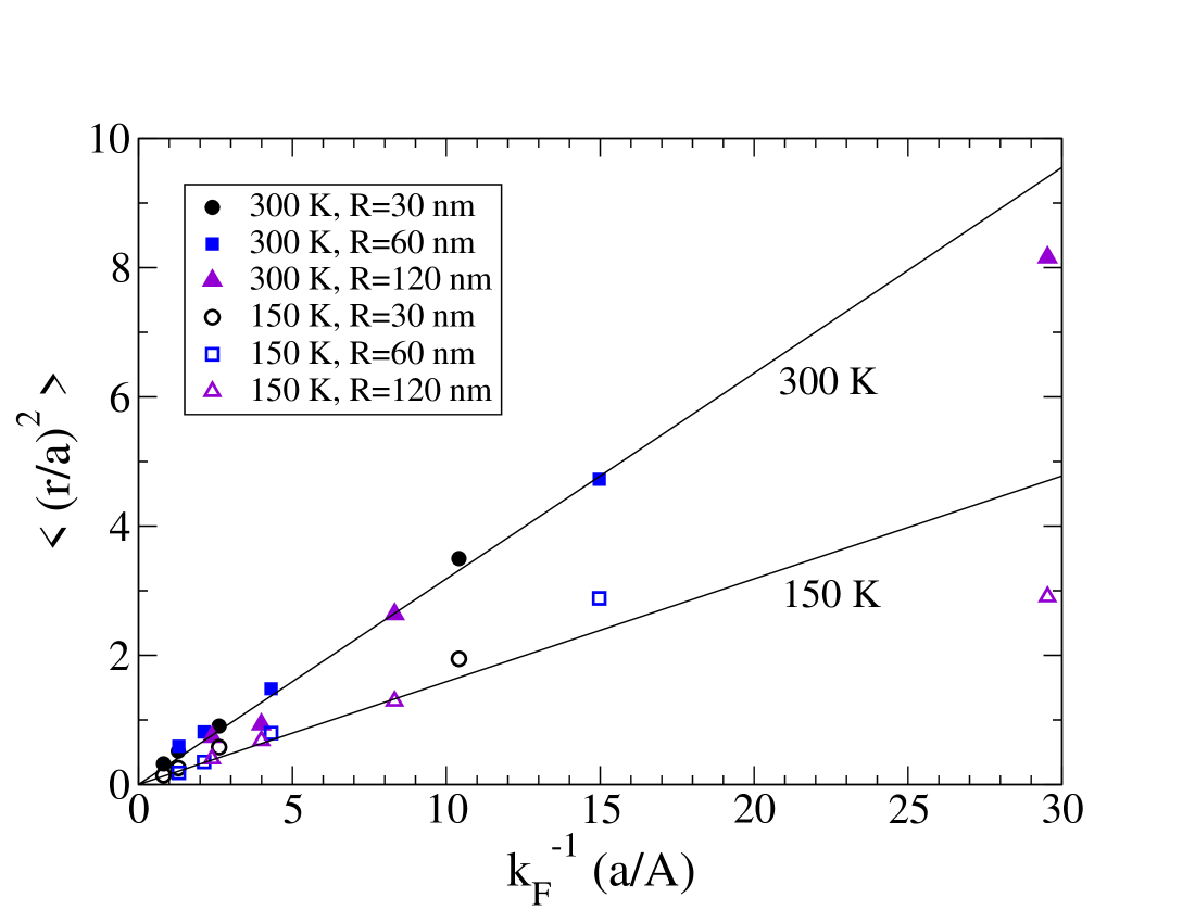
Figure 15: (Color online) Average squared displacement of the vortex core from the disk center, versus reciprocal force constant. The points come from simulations out to time $\tau=2.5\times 10^{5}$; the solid lines are the predictions from the equipartition theorem, Eq. 72, using the parameters for Py.

In consideration of the classical statistical mechanics, the important fact here is that the Hamiltonian (65) has a dynamics due to only two coordinates ($X,Y$) appearing quadratically. Although the dynamic equations for $\dot{X}$ and $\dot{Y}$ must come from the Hamiltonian (66) of the equivalent 2D SHO, the phase space of the Thiele dynamics is more restricted, due to relation (64) between ${\bf P}$ and ${\bf X}$. This forces the Thiele phase space to be only two dimensional; this does not depend on the choice of the gauge. As an example of that reduction of the phase space, elliptical motions are present for the 2D SHO, while the zero-temperature Thiele dynamics has only circular orbits. As we are considering thermal equilibrium, each independent quadratic coordinate receives an average thermal energy of $\tfrac{1}{2}kT$. This gives the connection needed to predict the average RMS vortex displacement from the disk center. Specifically, for each vortex core coordinate,

$$\langle\tfrac{1}{2}k_{F}X^{2}\rangle=\langle\tfrac{1}{2}k_{F}Y^{2}\rangle=\tfrac{1}{2}kT.$$ (71)

Then the average squared displacement of the vortex from the disk center should be

$$\langle r^{2}\rangle=\langle X^{2}+Y^{2}\rangle=r_{\rm rms}^{2}=\frac{2kT}{k_{F}}.$$ (72)

These show that the average thermal energy in the vortex motion must be

$$\langle H({\bf X},{\bf P})\rangle=kT.$$ (73)

Therefore, we can check that these relations actually hold in the simulations. The average squared displacement should be proportional to the reciprocal of the force constant, with the same proportionality factor (twice the temperature) when disks of different geometries are considered. Some results for the average squared displacements versus reciprocal force constant in different geometries are given in Figure 15. The results depend on the behavior of the force constant with disk geometry, showing the importance of static calculations for understanding the statistical dynamics behavior. The simulation data have a general trend consistent with Eq. 72, but there are large fluctuations due to the finite time sequences used, which is more of a problem for the systems with small $k_{F}$.

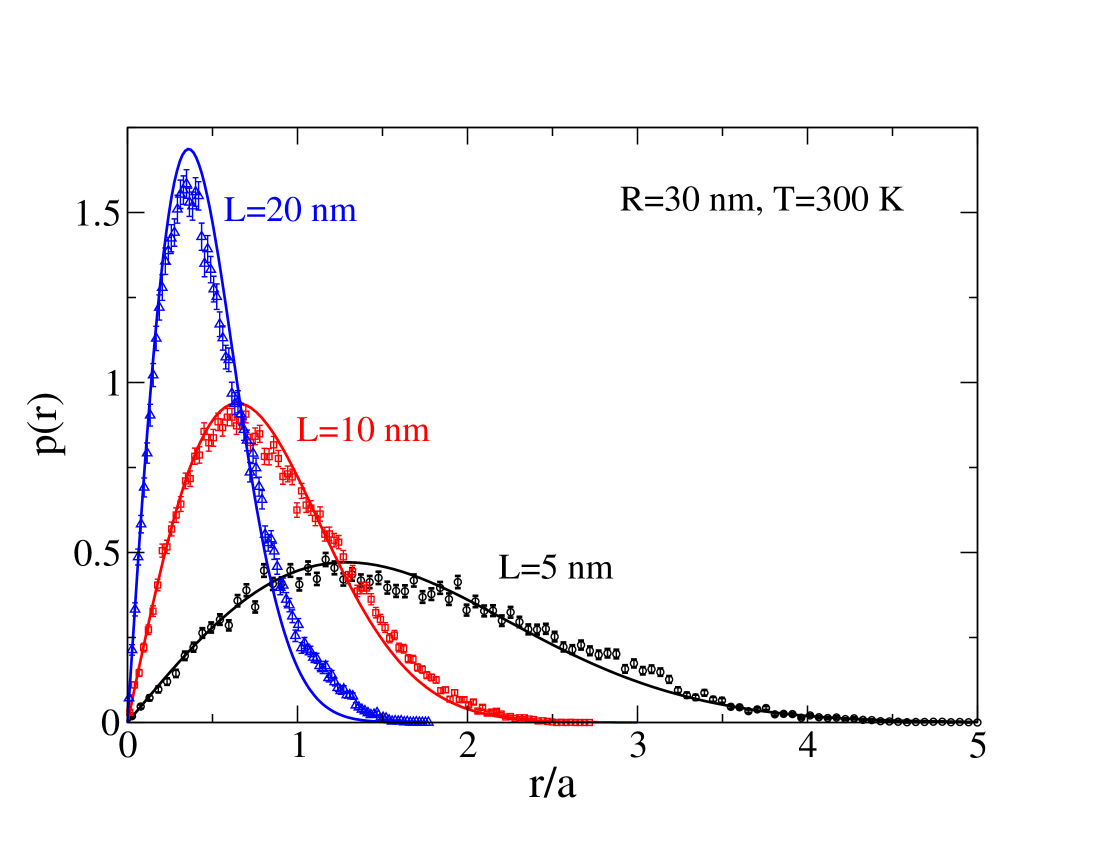
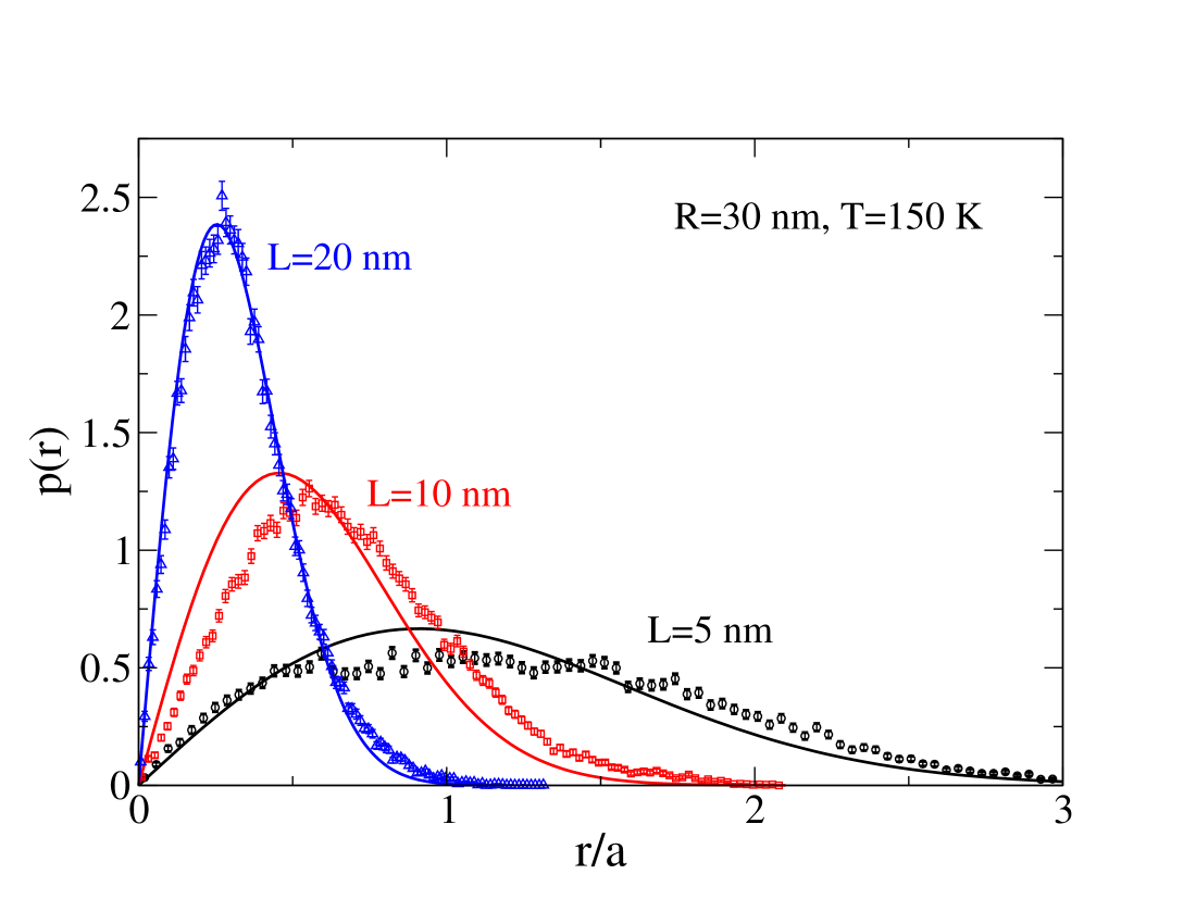
Figure 16: (Color online) Probability distributions in Py disks of radius 30 nm at temperatures 300 K and 150 K, for the radial position $r$ of the vortex, measured from the disk center, in units of the cell size, $a=2$ nm. Solid curves are the theoretical expression (74) based on a Boltzmann distribution using the static force constants; points are from simulations out to time $\tau=2.5\times 10^{5}$ .

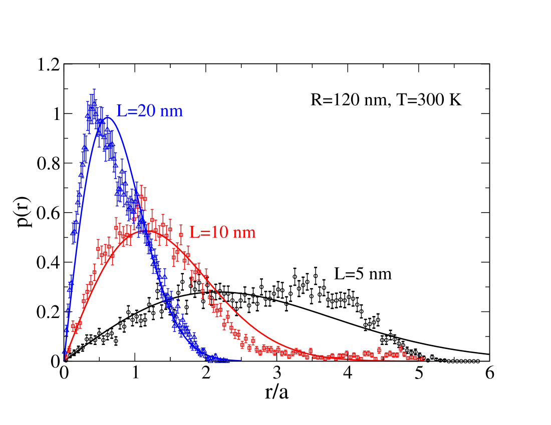
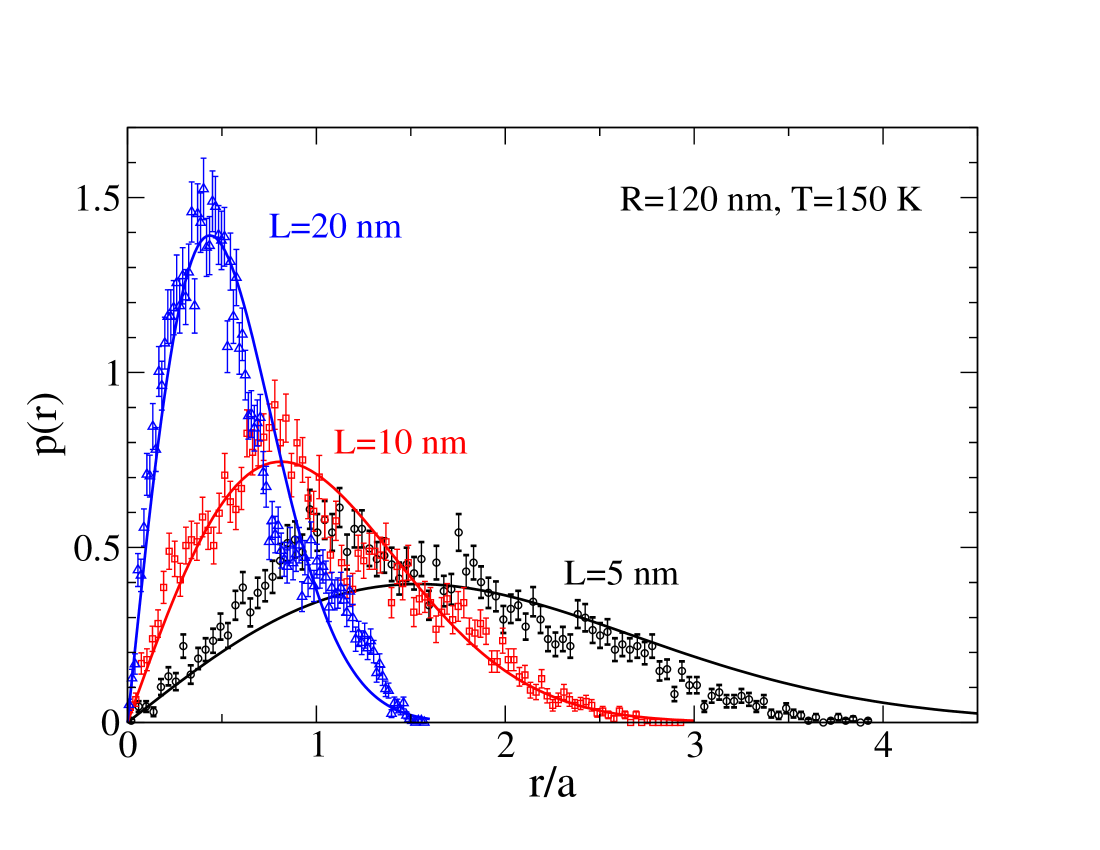
Figure 17: (Color online) Probability distributions for vortex radial position in Py disks of radius 120 nm, as explained in Figure 16.

We can further substantiate the statistical behavior of the vortex core, by calculating the probability distribution $p(r)$ of its distance $r=\sqrt{X^{2}+Y^{2}}$ from the disk center. Assuming that its position is governed by Boltzmann statistics for Hamiltonian (65), the normalized distribution from $p(r)dr\propto 2\pi r\,dr\,e^{-\beta H}$ is predicted to be

$$p(r)=\beta k_{F}r\,e^{-\frac{1}{2}\beta k_{F}r^{2}},$$ (74)

where $\beta=(kT)^{-1}$ is the inverse temperature. This distribution also has some particular distinctive points that are relatively easy to check. For instance, the distribution has a peak at the point of maximum probability, at the radius

$$r_{\rm max}=\sqrt{\frac{kT}{k_{F}}}=\frac{r_{\rm rms}}{\sqrt{2}}.$$ (75)

In addition, the value of the function at this point is

$$p_{\rm max}=p(r_{\rm max})=\frac{e^{-1/2}}{r_{\rm max}}.$$ (76)

We have found that the vortex core position satisfies this distribution reasonably well, while the vortex is undergoing the spontaneously generated gyrotropic motion. There is a certain difficulty to verify this, because very long time sequences (we used final time $\tau=250000$) are needed so that many gyrotropic revolutions are performed. During the motion, at times there are rather large fluctuations in the amplitude of the motion. The motion varies between time intervals of smooth gyrotropic motion of large amplitude and other time intervals where the motion seems to be impeded, and is of much smaller amplitude. Even so, we were able to take these long sequences and produce histograms of the vortex radial position to compare with the predicted probability distribution. An example for $R=30$ nm is given in Figure 16. The temperatures are defined here by applying the material parameters for Permalloy (that is, 300 K corresponds to $kT=0.1592Aa$, where the exchange stiffness for Py is $A=13$ pJ/m and cell size $a=2.0$ nm was used in all simulations). The data (points) are compared with the prediction of equation (74) (solid curves), for different disk thicknesses. For these smaller systems, the agreement is quite good between the simulations and the theoretical expression, Eq. (74).

The distributions were also found in simulations for larger radius, see Figure 17 for the distribution at $R=120$ nm. In this case, the errors are considerably greater. This is due primarily to the larger gyrotropic period. Over the sampling time interval to $\tau=2.5\times 10^{5}$, there are less periods being sampled. The system has a somewhat erratic behavior, in that the orbital radius of the vortex motion seems to switch suddenly between different values, as already mentioned. As a result, at this system size a greater time interval is needed to obtain a sample that could be considered in thermal equilibrium, with well defined averages.

For thinner disks, the number of revolutions in the given time interval is lesser, which means the thinner disks may also require longer time sequences to give the same relative errors. Of course, the thinner (thicker) disks have a weaker (stronger) force constant, leading to the greater (lesser) amplitude spontaneous motions. This is clearly exhibited in the probability distributions. Although these aspects may be difficult to verify experimentally, the results do indeed point to much stronger spontaneous gyrotropic fluctuations for very thin magnetic disks. In the cases where these motions were of greater amplitude, there may start to appear deviations from the distribution in (74), simply because the larger amplitude vortex motions cause the vortex to move out of the region where the potential is parabolic.

VI Discussion and conclusions

The calculations here give a precise description of the magnetostatics and dynamics for thin-film nanomagnets, especially in the situations where a single vortex is present. The continuum problem for some finite thickness $L$ has been mapped onto an equivalent 2D problem, i.e., the modified micromagnetics adapted here. For high aspect ratios, $L\ll 2R$, the shape anisotropy is very strong, and this 2D system is a very good approximation of the full 3D problem, because it leads to the physical situation where the magnetization has little dependence on $z$ and is predominately planar, except in the vortex core.

At zero temperature, we have been able to test this approach and compare with the predictions for vortex gyrotropic motion based on the Thiele equation. This comparison is made possible here because the vortex force constants $k_{F}$ can be calculated from the energetics of a vortex with a constrained position. The application of the Lagrange undetermined multipliers techniqueWysin2010 for enforcing a desired static vortex position ${\bf X}$ has been essential in the determination of $k_{F}$. In addition, that relaxation procedure also is of great utility for initiating a vortex at some radius while removing most of the initial spin wave like oscillations that would otherwise be generated when the time dynamics is started. As a result, we have been able to determine the zero temperature gyrotropic frequencies for the motion of the vortex core, ${\bf X}(t)$, to fairly high precision. The confirmation of the applicability of the Thiele equation to the $T=0$ dynamics of vortex velocity ${\bf V}$ is impressive, as demonstrated in the straight line fit for gyrotropic frequency $\omega_{G}$ versus scaled force constant $k_{F}/L$ in Figure 6. This shows the complete consistency between the statics calculations of the force constants and the dynamics calculations of the frequencies, when interpreted via the Thiele equation.

At larger disk radii, the gyrotropic frequency is found to be close to linear in the aspect ratio, $L/R$, see Eq. 58. The frequencies are also close to those found in the two-vortices model and micromagnetics calculations carried out in Ref. Guslienko++02, . The differences from those results may be due to the fact that we have used the cell parameter $a$ half of what was used in Ref. Guslienko++02, . This is important, because the cell parameter should be sufficiently less than the exchange length for results to be reliable. Otherwise, if $a$ is too large, the details of the energetics and dynamics in the vortex core cannot be correctly represented.

At $T>0$, the Langevin dynamics shows some surprising behavior that was reported earlier in Ref. Machado+11, , even when the vortex is initiated at the center of a nanodisk. The thermal fluctuations are indeed sufficiently strong to produce a spontaneous motion of the vortex core, without the application of any external field, which is not a simple random walk. Instead, the gyrotropic nature of the motion is still present, and in fact, persistent vortex rotation is the dominant feature of the motion. The thermal fluctuations can be viewed as a perturbation on top of the gyrotropic motion, however, it is the temperature that determines the expected squared radius of the orbit. The orbital radius is very well described from the statistical mechanics of the vortex collective coordinate Hamiltonian (65), that possesses only the potential energy associated with the vortex force constant.

Integrations of the dynamics over very long times (equivalent to hundreds of vortex revolutions) shows that the statistics of the vortex position follows the simple Boltzmann distribution in Eq. (74). The average squared vortex displacement from the origin, $r_{\rm rms}^{2}$, scales linearly in the temperature divided only by the force constant $k_{F}$. This is in contrast to the vortex gyrotropic frequencies, which depend on $k_{F}/L$. Thus, the results for force constant indirectly predict the expected position fluctuations. However, very long time sequences are needed to see this average behavior; over some short time intervals there can be large variations in the instantaneous vortex orbital radius. The largest spontaneous vortex position fluctuations will be possible in thin dots of larger radius, where the force constants are weakest. Even so, this is a small effect (RMS radii on the order of several nanometers), and it may be difficult to observe experimentally. As an example based only on the calculated force constants, a magnetic dot of radius $R=180$ nm and thickness $L=20$ nm has $k_{F}\approx 0.29A/a$. For Py at 300 K, this gives the estimate $r_{\rm rms}\approx 2.1$ nm. If the thickness is reduced to 10 nm, then $k_{F}\approx 0.080A/a$ and the RMS orbital radius increases to $r_{\rm rms}\approx 4.0$ nm. Even though these are rather small, the distributions $p(r)$ are rather wide and therefore at times one can expect even larger vortex gyrotropic oscillations.

Finally we note that the thermal distribution of the vortex rotational velocity is connected to the radial distribution $p(r)$, because the Hamilton equations (67) imply

$${\bf V}=\vec{\omega}_{G}\times{\bf X},\quad\vec{\omega}_{G}=-\frac{k_{F}}{G}\hat{z}.$$ (77)

Thus, we can transform magnitudes with $V=\omega_{G}r$. Then the RMS rotational velocity is

$$V_{\rm rms}=|\,\omega_{G}|\,r_{\rm rms}=\frac{\sqrt{2k_{F}\,kT}}{G},$$ (78)

which varies proportional to $\sqrt{k_{F}}/L$. This is connected to a Boltzmann distribution for the probability $f(V)\,dV$ of vortex speed $V$ in some interval of width $dV$, where

$$f(V)=\frac{p(V/\omega_{G})}{\omega_{G}}=\beta m_{G}Ve^{-\frac{1}{2}\beta m_{G}V^{2}}.$$ (79)

This involves a gyrotropic effective mass $m_{G}$,

$$\quad m_{G}\equiv\frac{G^{2}}{k_{F}}\approx\frac{(2\pi)^{2}}{0.878}\frac{R}{\mu_{0}\gamma^{2}},$$ (80)

determined both by the vortex force constant and by the disk thickness contained in the definition of $G$. For small aspect ratio, however, the thickness cancels and this mass is proportional to the disk radius alone. At $R=100$ nm, the mass is about $1.2\times 10^{-22}$ kg, independent of the material. Although $f(V)$ has a mathematical form identical to that for $p(r)$, it leads to another interesting interpretation of the vortex dynamics in equilibrium.

References

- (1) N.A. Usov and S.E. Peschany, J. Mag. Magn. Mater. 118, 290 (1993).
- (2) K.Yu. Guslienko, K.-S. Lee and S.-K. Kim, Phys. Rev. Lett. 100, 027203 (2008).
- (3) R.P. Cowburn, D.K. Koltsov, A.O. Adeyeye, M.E. Welland and D.M. Tricker, Phys. Rev. Lett. 83, 1042 (1999).
- (4) M. Schneider, H. Hoffmann and J. Zweck, Appl. Phys. Lett. 77, 2909 (2000).
- (5) J. Raabe, R. Pulwey, S. Sattler, T. Schweinbock, J. Zweck and D. Weiss, J. Appl. Phys. 88, 4437 (2000).
- (6) J.P. Park, P. Eames, D.M. Engebretson, J. Berezovsky and P.A. Crowell, Phys. Rev. B 67, 020403 (2003).
- (7) K.Yu. Guslienko, B.A. Ivanov, V. Novosad, Y. Otani, H. Shima and K. Fukamichi, J. App. Phys. 91, 8037 (2002).
- (8) K.Yu. Guslienko, X.F. Han, D.J. Keavney, R. Divan and S.D. Bader, Phys. Rev. Lett. 96, 067205 (2006).
- (9) A.R. Vólkel, F.G. Mertens, A.R. Bishop and G.M. Wysin, Phys. Rev. B43, 5992 (1991).
- (10) G.M. Wysin, F.G. Mertens, A.R. Völkel and A.R. Bishop, in Nonlinear Coherent Structures in Physics and Biology, p. 177, K.H Spatschek and F.G. Mertens, editors, (Plenum Press, New York, 1994) (ISBN 0306448033).
- (11) G.M. Wysin, Phys. Rev. B 54, 15156 (1996).
- (12) B.A. Ivanov, H.J. Schnitzer, F.G. Mertens and G.M. Wysin, Phys. Rev. B 58, 8464 (1998).
- (13) G.M. Wysin and A.R. Völkel, Phys. Rev. B 54, 12921 (1996).
- (14) K.L. Metlov and K.Yu. Guslienko, J. Mag. Magn. Mater. 242–245, 1015 (2002).
- (15) G.M. Wysin, J. Phys.: Condens. Matter 22, 376002 (2010).
- (16) A.A. Thiele, Phys. Rev. Lett. 30, 230 (1973).
- (17) D.L. Huber, Phys. Rev. B 26, 3758 (1982).
- (18) T.S. Machado, T.G. Rappoport and L.C. Sampaio, Appl. Phys. Lett. 100, 112404 (2012).
- (19) B.A. Ivanov et al., JETP Lett. 91, 178 (2010).
- (20) J.L. García-Palacios and F.J. Lázaro, Phys. Rev. B 58, 14937 (1998).
- (21) U. Nowak, in Annual Reviews of Computational Physics IX, p. 105, edited by D. Stauffer (World Scientific, Singapore, 2000).
- (22) Zhongyi Huang, J. Comp. Math. 21, 33 (2003).
- (23) D. Suessa, J. Fidler and T. Schrefl Handbook of Magn. Mater. 16 41 (2006).
- (24) G. Gioia and R.D. James Proc. R. Soc. London Ser. A 453 213 (1997).
- (25) C.J. García-Cervera, “Magnetic Domains and Magnetic Domain Walls,” Ph.D. thesis, New York University (1999).
- (26) C.J. García-Cervera, Z. Gimbutas and E. Weinan E J. Comp. Phys. 184 37 (2003).
- (27) G.M. Wysin, W.A. Moura-Melo, L.A.S. Mól and A.R. Periera, J. Phys.: Condens. Matter 24 296001 (2012).
- (28) J. Sasaki and F. Matsubara J. Phys. Soc. Japan 66, 2138 (1997).
- (29) George Marsaglia and Arif Zaman, Computers in Physics 8, No. 1, 117, (1994).
- (30) G.M. Wysin and F.G. Mertens, in Nonlinear Coherent Structures in Physics and Biology, Springer-Verlag Lecture Notes in Physics, M. Remoissenet and M. Peyrard, editors, (Springer-Verlag, Berlin, New York, 1991) (ISBN 0387548904).
- (31) K.Yu. Guslienko, V. Novosad, Y. Otani and K. Fukamichi, Appl. Phys. Lett. 78, 3848 (2001).
- (32) K.Y. Guslienko, A.N. Slavin, V. Tiberkevich, et al., Phys. Rev. Lett. 101, 247203 (2008).
- (33) C.E. Zaspel, B.A. Ivanov, P.A. Crowell, et al., Phys. Rev. B72, 024427 (2005).
- (34) B.A. Ivanov, E.G. Galkina and A.Yu. Galkin, Low Temp. Phys. 36, 747 (2010).