Collective Edge Modes of a Quantum Hall Ferromagnet in Graphene

Abstract

We derive an effective field-theoretical model for the one-dimensional collective mode associated with a domain wall in a quantum Hall ferromagnetic state, as realized in confined graphene systems at zero filling. To this end, we consider the coupling of a quantum spin ladder forming near a kink in the Zeeman field to the spin fluctuations of a neighboring spin polarized two-dimensional environment. It is shown, in particular, that such coupling may induce anisotropy of the exchange coupling in the legs of the ladder. Furthermore, we demonstrate that the resulting ferromagnetic spin-$1/2$ ladder, subject to a kinked magnetic field, can be mapped to an antiferromagnetic spin chain at zero magnetic field.

I Introduction

When an electron is confined within the lowest Landau level in a quantum Hall (QH) system, its position is described solely by the guiding center, whose X and Y coordinates do not commute with one another. Hence, the QH system can be formulated as a dynamical system in the noncommutative plane Prange1990 ; Sarma1997 . When the system supports discrete degrees of freedom, such as spin or layer index, for integrally filled Landau levels quantum coherence develops owing to the exchange interaction, and the system becomes ferromagnetic. The characteristic ground state is spin–polarized (or isospin-polarized, e.g. in bilayer QH systems), and single spin-flip excitations are not favored due to the large cost in exchange energy. Instead, the elementary excitation is a topological soliton named a Skyrmion Lee_1990 ; Sondhi_1993 ; Fertig_1994 ; Moon : a spin texture, where several spins are coherently rotated to lower the interaction energy. Skyrmions are indexed by a quantized topological charge – the Pontryagin number of the spin texture, associated also with a quantized electric charge. Indeed, the experimental detection of Skyrmions in QH systems realized in semiconductor devices Barett_1995 ; Leadley_1997 has provided compelling evidence for QH ferromagnetism.

In what follows, we study a two component quantum Hall system, with two Landau levels lying near the Fermi energy, with enough electrons to fill one of them. The effective Hamiltonian describing this quantum Hall ferromagnet (QHFM) is generally of the form

$$H_{\text{QHFM}}=J_{s}\int d^{2}r\big{[}\sum_{a=x,y,z}\big{|}\nabla\mathcal{S}_{a}(\textbf{r})\big{|}^{2}-\mathcal{B}(\textbf{r})\mathcal{S}_{z}(\textbf{r})\big{]};$$ (1)

here $\vec{\mathcal{S}}$ is the spin field (with $|\vec{\mathcal{S}}|=1/2$), and $J_{s}$ the spin stiffness determined by the exchange energy. The local, possibly nonuniform Zeeman field $\mathcal{B}(\textbf{r})$ encodes the noninteracting energy spectrum, which may include dispersion of the Landau levels due to boundaries or external potentials. Eq. (1) is actually a nonlinear sigma model with the O(3) symmetry broken down to O(2) symmetry. It supports a collective spin excitation, which is the Goldstone mode associated with the spontaneous symmetry breaking. Due to the association of the spin texture with electric charge Lee_1990 , this mode may carry charge and can therefore contribute to electric transport under certain circumstances Fertig and Brey (2006).

An interesting manifestation of collective states in a QHFM is expected in grapheneFertig and Brey (2006); Barlas2008 ; cote08 ; Zhao2010 . The Dirac dynamics of electrons near the the $\mathbf{K}$ and $\mathbf{K^{\prime}}$ points in the band structure dictates a unique, particle-hole conjugate spectrum of the Landau levels in the integer quantum Hall regime CastroNetoRMP . Most prominently, there exist zero energy Landau level states, responsible for unusual behavior of the $\nu=0$ QH state Abanin2007 ; Checkelsky . In monolayer graphene, the $\nu=0$ state possesses a four-fold degeneracy associated with the two valleys ($\mathbf{K}$ and $\mathbf{K^{\prime}}$) and the two spin states. The Zeeman coupling separates the states into two particle-hole conjugate pairs, above and below zero energy. In bilayer graphene, the layer index degree of freedom of the bilayer system further doubles the zero energy degeneracy, which can be lifted by applying a perpendicular electric field McCann2006 ; McCann2006a . When interactions are included, the half-filled zero energy states spontaneously polarize due to exchange, and give rise to a spin or valley polarized ferromagnetic ground state Zhang2006 ; Zhao2012 .

The unusual bulk spectrum of Landau levels in undoped graphene dictates an interesting structure of the edge states near the physical edge of a ribbon BreyFertig ; Abanin et al. (2006); Mazo , or at the interface between two opposite polarities of the gate voltage in a bilayer system Paramekanti . Most prominently, it gives rise to level crossings between an electron-like edge mode with a given spin or isospin state and a hole-like mode with the opposite spin/isospin state, localized on the same edge. This implies a spatial reversal in the direction of the effective Zeeman field, which in the presence of interactions induces a coherent domain wall (DW) between regions with distinct configurations of the QHFM ground state Fertig and Brey (2006); Huang . The resulting QHFM state is a realization of the model Eq. (1) with $\mathcal{B}(\textbf{r})=\mathcal{B}(x)$, in which $\mathcal{B}(x)$ changes sign across a line in the $xy$ plane. In this geometry, quantum fluctuations of the spin/isospin rotation angle support a collective edge mode, which possesses a one-dimensional (1D) dynamics. This edge mode has been argued to behave at low energies as a Luttinger liquid Fertig and Brey (2006); bilayerLL , or alternatively as an anti-ferromagnetic (AFM) spin chain Shimshoni2009 . However, an explicit derivation of the 1D effective model from the two-dimensional (2D) QHFM [Eq. (1)] has not been carried out in earlier literature beyond the semiclassical spin-wave approximation.

In the present paper, we consider a simple model for a 2D QHFM subject to a kink in the Zeeman field, which allows the derivation of an effective 1D quantum field-theoretical model for the dynamics of the collective DW mode along the kink. We find that within an appropriate regime of parameters, in particular assuming a sufficiently strong Zeeman field in the polarized regions, the low energy dynamics is equivalent to an AFM spin-$1/2$ chain, whose parameters can be systematically related to the original 2D system.

This paper is organized as follows: in Section II, we study the coupling of a single quantum spin ladder forming near a kink in the Zeeman field to the spin fluctuations of a neighboring spin polarized 2D environment. It is shown that the resulting effective 1D theory manifests anisotropy of the exchange coupling in the legs of the ladder. In Section III, we consider a ferromagnetic spin-$1/2$ zigzag ladder subject to a staggered magnetic field, and demonstrate its mapping to an antiferromagnetic spin chain at zero magnetic field. Finally, some concluding remarks are presented in Section IV.

II Derivation of a Quasi 1D Model for a Domain Wall

We consider a 2D electron system in a QHFM state, described by a discrete version of Eq. (1) where the lattice spacing between local spin operators is set by the average distance between electrons, proportional to the magnetic length $\ell_{B}=\sqrt{\hbar c/eB}$. The magnetic field $B_{z}({\bf r}=(x,y))$ is assumed to be independent of $y$, and to change sign across a narrow strip near $x=0$ as depicted in Fig. 1. The mean-field groundstate of this system contains an in-plane component to $\vec{\mathcal{S}}({\bf r})$ near $x=0$, so that the O(2) symmetry of the Hamiltonian is broken, and a gapless one-dimensional collective mode, propagating along the $y$-direction, is present. While quantum fluctuations restore the broken symmetry, the quasi-one-dimensional mode remains in the spectrum. Its dynamics, however, is affected by the ferromagnetic coupling to the bulk spins, composed of two semi-infinite planes each subject to a uniform magnetic field. Quantum fluctuations of these bulk spins act as an environment. Below we integrate over these degrees of freedom, to derive an effective model for the quasi 1D interface spin degrees of freedom.

For simplicity we focus on the square lattice model depicted in Fig. 1. Local spin $\frac{1}{2}$ operators at $|x|>x_{0}$, denoted $\sigma_{i,j}$, are subject to a constant magnetic field $B$, and spins at $-x_{0}<x<x_{0}$, denoted $\vec{S}_{i,j}$, are subject to a nonuniform magnetic field which changes linearly from $B$ to $-B$. We will consider only the left semi-infinite plane ($x<0$) and assume that $x_{0}\sim\ell_{B}$, so that the region $-x_{0}<x<0$ contains only a single chain of spins $\vec{S_{j}}$, subject to a uniform magnetic field $B_{1D}<<B$. The corresponding Hamiltonian is

$$H = H_{env}+H_{1D}+J^{\prime}\sum\limits_{j=-\infty}^{\infty}\vec{\sigma}_{0,j}\cdot\vec{S}_{j}\;,$$ (2)

$$H_{env} = J\sum\limits_{j=-\infty}^{\infty}\sum\limits_{i=0}^{\infty}\big{[}\vec{\sigma}_{i+1,j}\cdot\vec{\sigma}_{i,j}+\vec{\sigma}_{i,j+1}\cdot\vec{\sigma}_{i,j}\big{]}$$ (3)

$$- B\sum\limits_{j=-\infty}^{\infty}\sum\limits_{i=0}^{\infty}{\sigma}_{i,j}^{z}$$

$$H_{1D} = J^{\prime\prime}\sum\limits_{j=-\infty}^{\infty}\vec{S}_{j}\cdot\vec{S}_{j+1}-B_{1D}\sum\limits_{j=-\infty}^{\infty}{S}_{j}^{z}$$ (4)

where all couplings are ferromagnetic ($J,J^{\prime},J^{\prime\prime}<0$). (Note the labeling scheme used for $\sigma_{i,j}$ as depicted in Fig. 1.)

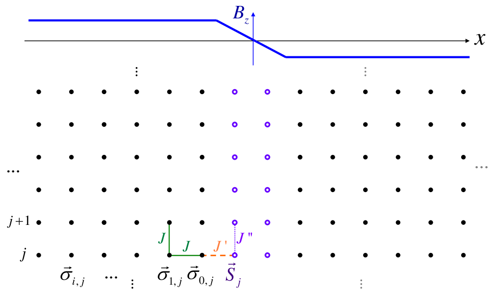
Figure 1: A symplified two dimensional system that consists of spins $\vec{\sigma}_{i,j}$ at high magnetic field and spins $\vec{S_{j}}$ at lower magnetic field.

Assuming the bulk magnetic field $B$ to be very high, a spin wave approximation can be used for the environmental spins $\vec{\sigma}_{i,j}$ assa :

$$\sigma_{i,j}^{z}\approx s_{0}-\frac{\left(\sigma_{i,j}^{x}\right)^{2}+\left(\sigma_{i,j}^{y}\right)^{2}}{2s_{0}}$$ (5)

where the total spin $s_{0}$ (with actual value $s_{0}=1/2$) is maintained as a parameter, playing the role of $\hbar$ in the canonical quantization of the spin fields in the $xy$-plane, which obey $[\sigma_{i,j}^{x},\sigma_{i,j}^{y}]=is_{0}$ in the spin-wave approximation. This yields the quadratic action for the isolated semi-infinite spin environment

$$S_{env}[\vec{\sigma}]=\int\limits_{0}^{\beta}d\tau\sum\limits_{j=-\infty}^{\infty}\sum\limits_{i=0}^{\infty}\,\Big{\{}\frac{i}{s_{0}}\sigma^{x}_{i,j}\partial_{\tau}\sigma_{i,j}^{y}+J\Big{(}{\sigma}_{i+1,j}^{x}{\sigma}_{i,j}^{x}$$

$$\qquad+{\sigma}_{i+1,j}^{y}{\sigma}_{i,j}^{y}+{\sigma}_{i,j+1}^{x}{\sigma}_{i,j}^{x}+{\sigma}_{i,j+1}^{y}{\sigma}_{i,j}^{y}\Big{)}$$

$$\quad\quad+\Big{(}\frac{1}{2s_{0}}B-2J\Big{)}\big{(}({\sigma}_{i,j}^{x})^{2}+({\sigma}_{i,j}^{y})^{2}\big{)}\Big{\}}$$

$$\quad\quad+\frac{J}{2}\int\limits_{0}^{\beta}d\tau\sum\limits_{j=-\infty}^{\infty}\,\big{(}({\sigma}_{0,j}^{x})^{2}+({\sigma}_{0,j}^{y})^{2}\big{)}$$ (6)

where $\vec{\sigma}=(\sigma^{x},\sigma^{y})$, and $\beta$ is the inverse temperature.

We next notice that the 1D spin chain $\vec{S}$ is coupled to the environment via the single chain $\vec{\sigma}_{0}$, whose effective 1D action can be expressed as

$$S_{env}^{1D}[\vec{\sigma}_{0}]=S^{SW}[\vec{\sigma}_{0}]+\delta S[\vec{\sigma}_{0}]\;,$$ (7)

where

$$S^{SW}[\vec{\sigma}_{0}]=\int\limits_{0}^{\beta}d\tau\sum\limits_{j}\big{[}\frac{i}{s_{0}}\sigma_{0,j}^{x}\partial_{\tau}\sigma_{0,j}^{y}+J\vec{\sigma}_{0,j}\cdot\vec{\sigma}_{0,j+1}$$

$$\qquad+\frac{1}{2s_{0}}B\big{(}({\sigma}_{0,j}^{x})^{2}+({\sigma}_{0,j}^{y})^{2}\big{)}\big{]}$$ (8)

and $\delta S$ is obtained after trace over the remaining environmental spins $\vec{\sigma}_{i\geq 1}$:

$$e^{-\delta S[\vec{\sigma}_{0}]}=\int D\vec{\sigma}_{i\geq 1}\,e^{-S_{env}[i\geq 1]}e^{-S_{env}[0,1]}\;.$$ (9)

Here $S_{env}[i\geq 1]$ schematically denotes the part of $S_{env}[\vec{\sigma}]$ describing the spins $\vec{\sigma}_{i,j}$ with $i\geq 1$, and $S_{env}[0,1]$ contains the interactions between spins $\vec{\sigma}_{0,j}$ and $\vec{\sigma}_{1,j}$.

To carry out the integration, we wish to use a Fourier representation of the spin wave fields. Since the semi-infinite plane imposes inconvenient boundary conditions, we employ a duplication of the chains $i\geq 1$ via the relation

$$e^{-2\delta S[\vec{\sigma}_{0}]}=e^{S^{SW}[\vec{\sigma}_{0}]}\int D\vec{\sigma}_{i\not=0}\,e^{-S_{2D}[\vec{\sigma}]}$$ (10)

where $S_{2D}[\vec{\sigma}]$ describes the spin-wave action of a full 2D lattice, in the presence of a constant Zeeman field $B$. The spins $\vec{\sigma}_{0}$ are excluded from the integration in Eq. (10). To enforce this constraint, we introduce Lagrange multipliers in terms of an auxiliary field $\vec{\lambda}$, yielding

$$e^{-2\delta S[\vec{\sigma}_{0}]}=e^{S^{SW}[\vec{\sigma}_{0}]}\int D\vec{\lambda}\,e^{-i\sum\limits_{{k_{y}},\omega_{n}}\vec{\lambda}^{T}({-k_{y}},-\omega_{n})\vec{\sigma}_{0}({k_{y}},\omega_{n})}$$ (11)

$$\quad\times\int D\vec{\sigma}\,e^{i\sum\limits_{{k}_{y},\omega_{n}}\vec{\lambda}^{T}({-k}_{y},-\omega_{n})\vec{\sigma}({k}_{y},\omega_{n})-S_{2D}[\vec{\sigma}]}$$

where we have used the Fourier transforms

$$\vec{\sigma}_{i,j}(\tau) = \frac{1}{\sqrt{N_{x}N_{y}\beta}}\sum_{\vec{k},\omega_{n}}e^{i(\vec{k}\cdot\vec{R}_{i,j}-\omega_{n}\tau)}\vec{\sigma}(\vec{k},\omega_{n})\;,$$

$$\vec{R}_{i,j} = a(i\,\hat{x}+j\,\hat{y})\;,$$

$$\vec{\lambda}_{j}(\tau) = \frac{1}{\sqrt{N_{y}\beta}}\sum_{k_{y},\omega_{n}}e^{i(k_{y}R_{j}-\omega_{n}\tau)}\vec{\lambda}(k_{y},\omega_{n})$$ (12)

(with $N_{x}$, $N_{y}$ the total number of sites in the corresponding directions). The bulk action in Eq. (11) can be expressed in terms of these fields as

$$S_{2D}[\vec{\sigma}]=\frac{1}{2s_{0}}\sum_{\vec{k},\omega_{n}}\vec{\sigma}^{T}(-\vec{k},-\omega_{n})G_{2D}^{-1}(\vec{k},\omega_{n})\vec{\sigma}(\vec{k},\omega_{n})$$ (13)

with

$$G_{2D}^{-1}(\vec{k},\omega_{n}) = \left(\begin{array}[]{cc}\omega_{2D}(\vec{k})&-\omega_{n}\\ \omega_{n}&\omega_{2D}(\vec{k})\end{array}\right)\;,$$ (16)

$$\omega_{2D}(\vec{k}) = 2Js_{0}\big{[}\cos(k_{x})+\cos(k_{y})-2\big{]}+B$$

$$\cong |J|s_{0}|\vec{k}|^{2}+B,$$

where $\vec{k}$ is in units of $1/a$, and in the last step we have used the long wavelength approximation $|\vec{k}|\ll 1$. After integration (see Appendix A for details) and substitution in Eq. (7), we obtain

$$\delta S_{env}^{1D}[\vec{\sigma}_{0}]=\frac{1}{2s_{0}}\sum\limits_{{k_{y}},i\omega_{n}}\vec{\sigma}_{0}(-{k_{y}},-\omega_{n})^{T}(G_{env}^{1D}({k_{y}},\omega_{n}))^{-1}\vec{\sigma}_{0}({k_{y}},\omega_{n})\;,$$ (17)

$$(G_{env}^{1D}({k_{y}},\omega_{n}))^{-1}\equiv\frac{1}{2}\left(\begin{array}[]{cc}-i|J|s_{0}(k_{-}+k_{+})+\omega_{sw}(k_{y})&|J|s_{0}(k_{+}-k_{-})-\omega_{n}\\ \\ -|J|s_{0}(k_{+}-k_{-})+\omega_{n}&-i|J|s_{0}(k_{-}+k_{+})+\omega_{sw}(k_{y})\\ \\ \end{array}\right)$$ (22)

where

$$k_{\pm} = i\sqrt{k_{y}^{2}+\frac{(B\pm i\omega_{n})}{|J|s_{0}}}\cong i\sqrt{\frac{B}{|J|s_{0}}}+\frac{i}{2}\sqrt{\frac{|J|s_{0}}{B}}k_{y}^{2}\mp\frac{\omega_{n}}{2\sqrt{B|J|s_{0}}}\;,$$ (23)

$$\omega_{sw}(k_{y}) = 2Js_{0}[\cos(k_{y})-1]+B\cong|J|s_{0}k_{y}^{2}+B\;.$$

Inserting the last approximations in Eq. (17), we note that the resulting effective action of the spin chain $\vec{\sigma}_{0}$ has the form of a semiclassical spin-wave theory in 1D with renormalized parameters:

$$\tilde{s}_{0} = s_{0}\left(\frac{2}{1+\alpha}\right)\;,\quad\tilde{J}=J\left(\frac{1+\alpha}{2}\right)\;,$$

$$\tilde{B} = B\left(\frac{1+2\alpha}{1+\alpha}\right)\;,\quad{\rm with}\quad\alpha\equiv\sqrt{\frac{|J|s_{0}}{B}}\;.$$ (24)

The fractional renormalization of the spin magnitude $s_{0}$ is a signature for the deviation from a pure spin Hamiltonian dynamics, arising from the trace over environmental degrees of freedom.

We are finally ready to derive the effective action for the spin chain $\vec{{S}}$, obtained after integration over the spins $\vec{\sigma}_{0}$:

$$e^{-S_{eff}[\vec{S}]} = e^{-S_{0}[\vec{S}]-\delta S_{eff}[\vec{S}]}$$

$$= e^{-S_{0}[\vec{S}]}\int D\vec{\sigma}_{0}\,e^{-S_{int}[\vec{\sigma}_{0},\vec{S}]-S_{env}^{1D}[\vec{\sigma}_{0}]}\;,$$

in which $S_{int}[\vec{\sigma}_{0},\vec{S}]$ describes the coupling between the two chains, associated with the last term in Eq. (2). Since we wish to account for the full quantum mechanical nature of the spin operators $\vec{{S}}$, a spin-wave approximation of the latter is avoided. Hence, a convenient representation of $S_{eff}[\vec{S}]$ in Fourier space is not available. To facilitate a coherent states path-integral formulation, we therefore map the spin operators to interacting fermions via the Jordan-Wigner (JW) transformation giamarchi

$$S_{j}^{+}=c_{j}^{\dagger}e^{i\pi\sum\limits_{i<j}c_{i}^{\dagger}c_{i}}\;,\;S_{j}^{-}=e^{-i\pi\sum\limits_{i<j}c_{i}^{\dagger}c_{i}}c_{j}$$

$$S_{j}^{z}=c_{j}^{\dagger}c_{j}-\frac{1}{2}\;.$$ (26)

Within a spin-wave approximation for the spin fields $\vec{\sigma}_{0}$, the interaction Hamiltonian acquires the form

$$H_{int}[\vec{\sigma_{0}},\vec{S}]=J^{\prime}\sum\limits_{j}\left\{\frac{1}{2}(\sigma_{0}^{+}e^{-i\pi\sum\limits_{i<j}c_{i}^{\dagger}c_{i}}c_{j}+c_{j}^{\dagger}e^{i\pi\sum\limits_{i<j}c_{i}^{\dagger}c_{i}}\sigma_{0}^{-})+s_{0}(c_{j}^{\dagger}c_{j}-\frac{1}{2})\right\}$$ (27)

where $\sigma^{\pm}_{0}=(\sigma_{0}^{x}\pm i\sigma_{0}^{y})$. The last term describes a simple shift of the Zeeman field (i.e., a chemical potential of the JW fermions). However the coupling of the spin wave fields $\sigma^{\pm}_{0}$ to the JW fermions is highly non-local and non-linear. Introducing the variables

$$\bar{\mathcal{S}}(j,\tau)=\bar{\psi}_{j}e^{i\pi\sum\limits_{i<j}\bar{\psi}_{i}\psi_{i}}$$ (28)

and its complex conjugate $\mathcal{S}$, which represent the spins in terms of the Grassmann variables $\psi_{j}$, $\bar{\psi}_{j}$, and performing the integration in Eq. (II), we find the correction to the action of 1D chain of spins $\vec{S}$ (see Appendix B for details):

$$\delta S_{eff}[\vec{S}]=\int d\tau d\tau^{\prime}\sum\limits_{j,j^{\prime}}\,\left\{\bar{\mathcal{S}}(j,\tau)V_{eff}(j,j^{\prime};\tau,\tau^{\prime})\mathcal{S}(j^{\prime},\tau^{\prime})+c.c.\right\}+J^{\prime}\int d\tau\sum\limits_{j}\,(\bar{\psi}_{j}(\tau)\psi_{j}(\tau)-\frac{1}{2})\;,$$ (29)

$$V_{eff}(j,j^{\prime};\tau,\tau^{\prime})=-\frac{J^{\prime 2}\tilde{s_{0}}}{8}\frac{1}{\sqrt{\pi|J|s_{0}(\tau-\tau^{\prime})}}e^{-\tilde{B}(\tau-\tau^{\prime})}e^{-\frac{(j-j^{\prime})^{2}}{4|J|s_{0}(\tau-\tau^{\prime})}}\Theta(\tau-\tau^{\prime})$$ (30)

where the parameters $\tilde{s_{0}}$ and $\tilde{B}$ are defined in Eq. (II).

The effective interaction term in Eq. (30) appears to be hardly useful in its exact form. However, it should be noticed that $V_{eff}$ decays exponentially for $(\tau-\tau^{\prime})>1/\tilde{B}$. As long as one is interested in physical properties (e.g., spin-spin correlations) in the long length scale limit (or, equivalently, for low temperatures $T\ll\tilde{B}$), $V_{eff}$ may be treated as almost local in imaginary time. In addition, it is short-range in space: the Gaussian factor decays on length scales

$$\tilde{a}\sim a\sqrt{|J|s_{0}(\tau-\tau^{\prime})}\sim\alpha a$$

[$\alpha$ defined in Eq. (II)], i.e. the short distance cutoff is normalized by a constant factor. For $J^{\prime}<\tilde{B}$, one obtains a converging perturbation series which indicates that $\delta S_{eff}$ is a marginal operator under renormalization group (RG). Its contribution therefore amounts to additive corrections to parameters of the standard terms in the bare action of the quantum spin chain, $S_{0}$.

The most obvious correction induced by $\delta S_{eff}$ is the modification of the Zeeman field due to the mean–field polarization of the environmental spins: $B_{1D}\rightarrow B_{1D}+|J^{\prime}|s_{0}$. More interestingly, the exchange coupling in the $xy$-plane is modified: $J^{\prime\prime}_{xy}\rightarrow J^{\prime\prime}_{xy}+\delta J_{xy}$, where

$$\delta J_{xy}\sim-\frac{J^{\prime 2}}{\tilde{B}}\frac{\tilde{s_{0}}}{4}=-\frac{J^{\prime 2}}{\sqrt{B}(2\sqrt{|J|s_{0}}+\sqrt{B})}\;.$$ (31)

Since $J^{\prime\prime}_{z}$ is unchanged, this implies that anisotropy is induced in the $xy$-plane. As the bare Heisenberg exchange is ferromagnetic ($J^{\prime\prime}<0$), the negative correction $\delta J_{xy}$ leads to enhancement of $J^{\prime\prime}_{xy}$ compared to $J^{\prime\prime}_{z}$. As a result, the effective low-energy model for the spin chain is the XXZ model, in the regime where its dynamics is governed by a Luttinger liquid Hamiltonian with a finite Luttinger parameter $K>1$. As discussed in the next Section, this enables the application of Bosonization for the study of its quantum dynamics when coupled to a second chain on the right hand side of $x=0$ (see Fig. 1).

III Mapping to AFM Spin Chain

In the previous section we considered only half of the space, and by integrating out reservoir degrees of freedom we arrived at a one dimensional spin chain with renormalized couplings. A similar procedure applied to the second half-space yields a parallel spin-chain with identical exchange parameters, but an opposite sign of the effective magnetic field. The two chains are coupled via ferromagnetic exchange interactions. We thus obtain an effective ferromagnetic spin-$1/2$ ladder, subject to a magnetic field which has opposite sign on the two legs, and therefore tends to frustrate the ferromagnetic interactions.

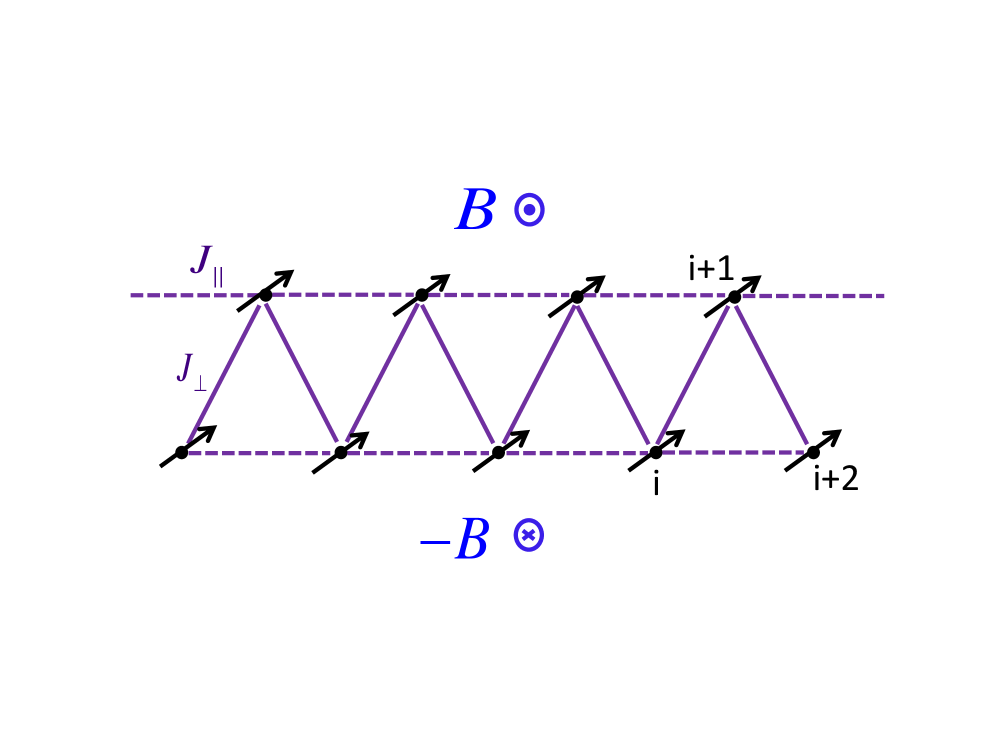
Figure 2: Ferromagnetic zigzag spin ladder subject to a staggered magnetic field $B$. Transverse exchange coupling ($J_{\perp}$) and longitudinal exchange coupling ($J_{\parallel}$) are represented by full and dashed bonds, respectively.

To study the dynamics of such a system, we focus on the simplest version of a ladder which possesses a zigzag structure (see Fig. 2). To this end, we consider the following model:

$$H=H_{\perp}+H_{\parallel}+H_{mag}\;,$$

$$H_{\perp}=-\frac{1}{2}|J_{\perp}^{xy}|\sum\limits_{i}\big{[}S^{+}_{i}S^{-}_{i+1}+S^{-}_{i}S^{+}_{i+1}\big{]}-|J_{\perp}^{z}|\sum\limits_{i}S^{z}_{i}S^{z}_{i+1}$$

$$H_{\parallel}=-\frac{1}{2}|J_{\parallel}^{xy}|\sum\limits_{i}\big{[}S^{+}_{i}S^{-}_{i+2}+S^{-}_{i}S^{+}_{i+2}\big{]}-|J_{\parallel}^{z}|\sum\limits_{i}S^{z}_{i}S^{z}_{i+2}$$

$$H_{mag}=-B\sum\limits_{i}(-1)^{i}S_{i}^{z}\;,$$ (32)

where even and odd sites $i$ are located on the top and bottom legs of the ladder, respectively. The zigzag ladder is thus represented as a single chain with nearest and next nearest neighbor interactions, subject to a staggered magnetic field $B$. Using the Jordan-Wigner transformation [Eq. (26)] and a subsequent bosonization of the fermion fields in the continuum limit giamarchi

$$\psi(x)=\psi_{R}+\psi_{L}$$

$${\rm where}\quad\psi_{R,L}=\frac{1}{{\sqrt{2\pi a}}}e^{\pm ik_{F}x}e^{i(\mp\phi+\theta)}$$ (33)

(in which $\phi$, $\theta$ obey the canonical commutation relations $[\phi(x),\partial_{x}\theta(x^{\prime})]=i\pi\delta(x^{\prime}-x)$, and $k_{F}=\pi/2a$), we obtain

$$H_{\perp}=\frac{1}{2\pi}\int dx\,\Big{[}u_{\perp}K_{\perp}(\nabla\theta)^{2}+\frac{u_{\perp}}{K_{\perp}}(\nabla\phi)^{2}\Big{]}$$

$$\qquad+\frac{|J_{\perp}^{z}|}{2\pi^{2}a}\int dx\,\cos(4\phi)$$

$$H_{\parallel}=\frac{1}{2\pi}\int dx\Big{[}u_{\parallel}K_{\parallel}(\nabla\theta)^{2}$$

$$\qquad+\frac{u_{\parallel}}{K_{\parallel}}(\nabla\phi)^{2}\Big{]}+\frac{|J_{\parallel}^{z}|}{2\pi^{2}a}\int dx\,\cos(4\phi)$$

$$H_{mag}=-\frac{B}{\pi a}\int dx\,\cos(2\phi)\;.$$

Here the velocities $u_{\perp}$, $u_{\parallel}$ and the Luttinger parameters $K_{\perp}$, $K_{\parallel}$ are dictated by the values of $J_{\perp}^{\alpha}$, $J_{\perp}^{\alpha}$. For $|J^{z}|\ll|J^{xy}|$,

$$u_{\perp}K_{\perp}=v_{F}^{\perp}=|J^{xy}_{\perp}|a$$ (34)

$$\qquad\frac{u_{\perp}}{K_{\perp}}=v_{F}^{\perp}-\frac{4|J^{z}_{\perp}|a}{\pi}$$

$$u_{\parallel}K_{\parallel}=\frac{u_{\parallel}}{K_{\parallel}}=0\;.$$

More generally, the Hamiltonian can be written as

$$H=\frac{1}{2\pi}\int dx\,\Big{[}uK(\nabla\theta)^{2}+\frac{u}{K}(\nabla\phi)^{2}\Big{]}$$ (35)

$$\qquad+\frac{|J_{\perp}^{z}|+|J_{\parallel}^{z}|}{2\pi^{2}a}\int dx\,\cos(4\phi)-\frac{B}{\pi a}\int dx\,\cos(2\phi)$$

where

$$uK=u_{\perp}K_{\perp}+u_{\parallel}K_{\parallel}\qquad\quad\frac{u}{K}=\frac{u_{\perp}}{K_{\perp}}+\frac{u_{\parallel}}{K_{\parallel}}\;.$$ (36)

The first term is a Luttinger liquid, with a Luttinger parameter given by

$$K=\sqrt{\frac{u_{\perp}K_{\perp}+u_{\parallel}K_{\parallel}}{\frac{u_{\perp}}{K_{\perp}}+\frac{u_{\parallel}}{K_{\parallel}}}}\;.$$ (37)

Note that in any case $K>1$, characteristic of a ferromagnetic XXZ spin-chain.

We now consider the effect of the non-linear terms in Eq. (35). Since the scaling dimension of an operator of the form $\cos(n2\phi)$ is $\Delta_{n}=n^{2}K$ (see, e.g., Ref. giamarchi, ), the $\cos(4\phi)$ term is less relevant and can be ignored. The Hamiltonian therefore reduces to a sine-Gordon model, where the $\cos(2\phi)$ induced by the staggered field becomes relevant when $K$ is tuned below $K_{c}=2$.

It is interesting to note that the model can be mapped to the continuum limit of an antiferromagnetic (AFM) spin-chain model by rescaling the fields $\phi$, $\theta$ and the parameter $K$ as follows:

$$\tilde{\phi}=\frac{1}{2}\phi\qquad\qquad\tilde{\theta}=2\theta\qquad\qquad\tilde{K}=\frac{1}{4}K\;.$$ (38)

In terms of the new fields,

$$H=\frac{1}{2\pi}\int dx\,\Big{[}u\tilde{K}(\nabla\tilde{\theta})^{2}+\frac{u}{\tilde{K}}(\nabla\tilde{\phi})^{2}\Big{]}$$ (39)

$$\qquad-g\int dx\,\cos(4\tilde{\phi})$$

where $g=\frac{B}{\pi a}$. For $K<4$, one obtains $\tilde{K}<1$ and the model Eq. (39) can be interpreted as an effective antiferromagnetic XXZ spin-chain. Tuning the original Luttinger parameter below $K_{c}=2$ corresponds to $\tilde{K}<1/2$, where the cosine term becomes relevant and a spin gap is opened, as proposed in Ref. Shimshoni2009, . In the ordered (gapped) phase, $S_{z}$ is polarized by the staggered field forming a staggered pattern on the zigzag chain, which indeed is equivalent to AFM ordering.

IV Summary

The unique spectral properties of electrons in undoped graphene provide a possibility to realize and control spin-textures and domain walls, forming near a kink-like structure in the effective magnetic field. Quantum fluctuations of the spin configuration dictated by such a kink are manifested by the presence of an effectively 1D collective mode, which propagates along the DW (i.e., in the translationally invariant direction). Its quantum dynamics is governed by a competition between the interaction-induced ferromagnetism and the staggered polarization of the Zeeman field across the DW. Projecting the spin-wave theory of the 2D QHFM onto the low energy 1D mode, one obtains a quadratic approximation for the dynamics in terms of an effective Luttinger liquid model Fertig and Brey (2006). However, a field-theoretical description beyond the Gaussian level should account for the fact that, due to the vanishing of the polarizing field at the center of the DW, a semiclassical spin-wave approximation is not well-justified.

As described in the previous sections, in this paper we suggest an alternative prescription for the derivation of an effective field theory which does not fully rely on a Gaussian spin-wave approximation. We have demonstrate the possible consequences of this prescription by studying a toy model, where the full quantum dynamics of the central region of the DW is modeled by a quasi 1D spin-$1/2$ system, coupled to the spin wave fluctuations of the remaining (almost polarized) 2D ferromagnetic environment. Generally, the resulting effective 1D field theory obtained by integrating over the environmental degrees of freedom [encoded by a correction to the action Eqs. (29), (30)] is quite complex, being non-local in both space and imaginary time. This is a manifestation of the fact that the effective action can not be derived from a pure Hamiltonian dynamics of the spin system. It is interesting to note that in the long wave-length limit, the effective 1D theory describing the boundary layer of the environment [see Eqs. (17) through (II)] can be formally mapped to a “standard” action of a spin system with renormalized (non-quantized) spin magnitude, $s_{0}\rightarrow\tilde{s_{0}}$. Assuming $|J|s_{0}<B$ (which guarantees the validity of the spin-wave approximation in the 2D environment), it is implied that the spin magnitude is enlarged ($\tilde{s_{0}}>s_{0}$). This can be interpreted as an effective suppression of $\hbar$: indeed, the coupling to a polarized QHFM environment stiffens the quantum fluctuations in the DW, turning its dynamics to a more “classical” one.

Despite the general complexity of the above mentioned effective field-theory, the presence of a high energy scale $\tilde{B}$ characterizing the gap for spin fluctuations in the environment [cf. Eq. (30)] implies that $\delta S_{eff}$ has a very good local approximation. This allows a mapping of the low-energy dynamics of the DW in its final form to a standard spin-$1/2$ ladder model, with renormalized parameters dictated by the coupling to the environment. In particular, the effective Zeeman field on each side of the DW center is enhanced due to the local field imposed by the environment, and anisotropy is introduced due to an effective enhancement of the exchange coupling in the $xy$-plane. We finally arrive at a sine-Gordon model [Eq. (35), or equivalently Eq. (39)] which reflects the competition between these two effects. This reflects the possibility to obtain a quantum phase transition from Luttinger liquid behavior (encoded by the quadratic approximation) to an ordered phase with a spin gap. Recalling that the operator $S_{z}$ can be traced back to electric current fluctuations Abanin et al. (2006); Shimshoni2009 , the physical interpretation of this ordered state is that of a perfect conductor: right-moving and left-moving channels (propagating along the DW) are localized in the transverse direction at opposite sides of the DW center, and backscattering is inhibited. A possible relation of this physics to transport in single layer graphene in the QH regime has been discussed elsewhere Shimshoni2009 .

Appendix A Derivation of the effective 1D environmental Green’s function

To evaluate $\delta S_{env}^{1D}[\vec{\sigma}_{0}]$ (Eq. (11)), we first perform the integration over the 2D spin fields $\vec{\sigma}$

$$Z[\vec{\lambda}]\equiv\int D\vec{\sigma}\,e^{i\sum\limits_{{k}_{y},\omega_{n}}\vec{\lambda}^{T}({-k}_{y},-\omega_{n})\vec{\sigma}({k}_{y},\omega_{n})-S_{2D}[\vec{\sigma}]}\;,$$ (40)

noting that

$$\vec{\sigma}(k_{y},\omega_{n})=\frac{1}{\sqrt{N_{x}}}\sum_{k_{x}}\vec{\sigma}(\vec{k},\omega_{n})\;.$$ (41)

Using Eq. (13) for $S_{2D}[\vec{\sigma}]$, the Gaussian integration yields

$$Z[\vec{\lambda}]=e^{-\frac{s_{0}}{2}\sum\limits_{{k_{y}},\omega_{n}}\vec{\lambda}({-k_{y}},-\omega_{n})^{T}G^{1D}({k_{y}},\omega_{n})\vec{\lambda}({k_{y}},\omega_{n})}$$ (42)

in which

$$G^{1D}({k_{y}},\omega_{n})\equiv\frac{1}{N_{x}}\sum_{k_{x}}G_{2D}(\vec{k},\omega_{n})\;,$$ (43)

and $G_{2D}(\vec{k},\omega_{n})$ is obtained by inverting Eq. (16). The resulting diagonal elements of $G^{1D}$ are therefore given by

$$G^{1D}_{1,1}=G^{1D}_{2,2}=a\int\frac{dk_{x}}{2\pi}\,\frac{\omega_{2D}(\vec{k})}{\omega^{2}_{2D}(\vec{k})+\omega_{n}^{2}}$$ (44)

$$\cong\frac{a}{2}\int\frac{dk_{x}}{2\pi}\,\Big{\{}\frac{1}{|J|s_{0}k^{2}+B+i\omega_{n}}+\frac{1}{|J|s_{0}k^{2}+B-i\omega_{n}}\Big{\}}$$

$$=\frac{a}{2}\frac{1}{|J|s_{0}}\int\frac{dk_{x}}{2\pi}\,\Big{\{}\frac{1}{k_{x}^{2}-k_{-}^{2}}+\frac{1}{k_{x}^{2}-k_{+}^{2}}\Big{\}}\;,$$

where $\displaystyle k_{\pm}=i\sqrt{k_{y}^{2}+\frac{1}{|J|s_{0}}(B\pm i\omega_{n})}$. After integration, we get

$$G^{1D}_{1,1}=G^{1D}_{2,2}=\frac{ia}{4}\frac{1}{|J|s_{0}}\Big{\{}\frac{1}{k_{+}}+\frac{1}{k_{-}}\Big{\}}$$

$$=\frac{ia}{4}\frac{1}{|J|s_{0}}\frac{k_{+}+k_{-}}{k_{+}k_{-}}\;.$$ (45)

Similarly, the off-diagonal components are given by

$$G^{1D}_{1,2}=-G^{1D}_{2,1}=a\int\frac{dk_{x}}{2\pi}\,\frac{\omega_{n}}{\omega^{2}_{2D}(\vec{k})+\omega_{n}^{2}}$$

$$\cong\frac{a}{4}\frac{1}{|J|s_{0}}\frac{k_{+}-k_{-}}{k_{+}k_{-}}\;.$$ (46)

Inserting $Z[\vec{\lambda}]$ from Eq. (42) (with $G^{1D}$ given by Eqs. (A), (A)) into Eq. (11), and integrating over $\vec{\lambda}$, we arrive at the final expression for the inverse Green’s function $(G_{env}^{1D}({k_{y}},\omega_{n}))^{-1}$, Eq.(17).

Appendix B Effective Action of the 1D spin-chain

In this Appendix, we detail the final stage of derivation of the correction to the effective action, $\delta S_{eff}[\vec{S}]$ (Eq. (29)), resulting from the interaction of the 1D spin-chain with the environment. Starting from Eq. (II), we first define the normalized complex field variables

$$\bar{\varphi}=\frac{1}{\sqrt{2\tilde{s_{0}}}}\sigma_{0}^{-}\qquad\qquad\varphi=\frac{1}{\sqrt{2\tilde{s_{0}}}}\sigma_{0}^{+}$$ (47)

describing the environmental spins $\vec{\sigma_{0}}$ within a spin-wave approximation. The integral over $\vec{\sigma_{0}}$ can therefore be written as

$$e^{-\delta S_{eff}[\vec{S}]}=\int D\varphi D\bar{\varphi}\,\text{exp}\Big{\{}-S_{int}[\vec{S},\varphi,\bar{\varphi}]-\sum\limits_{{k_{y}},\omega_{n}}\bar{\varphi}(-{k_{y}},-\omega_{n})(\tilde{B}+|\tilde{J}|\tilde{s_{0}}k_{y}^{2}-i\omega_{n})\varphi({k_{y}},\omega_{n})\Big{\}}$$ (48)

where, using Eq. (27),

$$S_{int}[\vec{S},\varphi,\bar{\varphi}]=J^{\prime}\sqrt{\frac{\tilde{s_{0}}}{2N_{y}\beta}}\sum\limits_{k_{y},\omega_{n}}\sum_{j}\int d\tau\,\big{(}\varphi(k_{y},\omega_{n})e^{ik_{y}j-i\omega_{n}\tau}\bar{\mathcal{S}}(j,\tau)+e^{-ik_{y}j+i\omega_{n}\tau}\mathcal{S}(j,\tau)\bar{\varphi}(k_{y},\omega_{n})\big{)}\;.$$ (49)

A straightforward Gaussian integration then yields

$$\delta S_{eff}[\vec{S}]=-\frac{J^{\prime 2}\tilde{s_{0}}}{8}\sum_{j,j^{\prime}}\int d\tau d\tau^{\prime}\,\bar{\mathcal{S}}(j,\tau)\frac{1}{N_{y}\beta}\sum\limits_{k_{y},\omega_{n}}e^{ik_{y}(j-j^{\prime})-i\omega_{n}(\tau-\tau^{\prime})}\frac{1}{\tilde{B}+|\tilde{J}|\tilde{s_{0}}k_{y}^{2}-i\omega_{n}}\mathcal{S}(j^{\prime},\tau^{\prime})\;.$$ (50)

Integrating over $k_{y}$ and $\omega_{n}$, we obtain the final expression for $\delta S_{eff}[\vec{S}]$ with the effective interaction $V_{eff}$ given by Eq. (30).

References

• (1) R.E. Prange and S. M. Girvin, eds., The Quantum Hall Effect (Springer-Verlag, New York, 1990).
• (2) S. Das Sarma and A. Pinczuk, eds., Perspectives in Quantum Hall Effects (John Wiley & Sons, 1997).
• (3) D.H. Lee and C.L. Kane, Phys. Rev. Lett. 64, 1313 (1990).
• (4) S.L. Sondhi, A.Karlhede, S.A. Kivelson and E. H. Rezayi, Phys. Rev. B 47, 16419 (1993).
• (5) H.A. Fertig, L Brey, R. Côt$\acute{e}$, A.H. MacDonald, Phys. Rev. B 50, 11018 (1994).
• (6) K. Moon, H. Mori, K. Yang, S. M. Girvin, A. H. MacDonald, L. Zheng, D. Yoshioka and S.-C. Zhang, Phys. Rev. B 51, 5138 (1995).
• (7) S.E. Barrett, G. Dabbagh, L. N. Pfeiffer, K. W. West and R. Tycko, Phys. Rev. Lett. 74, 5112 (1995).
• (8) D.R. Leadley, R. J. Nicholas, D. K. Maude, A. N. Utjuzh, J. C. Portal, J. J. Harris and C. T. Foxon, Phys. Rev. Lett. 79, 4246 (1997).
• Fertig and Brey (2006) H. A. Fertig and L. Brey, Phys. Rev. Lett. 97, 116805 (2006).
• (10) Y. Barlas, R. Cote, K. Nomura, and A. H. MacDonald, Phys. Rev. Lett. 101, 097601 (2008).
• (11) R. Coté, J.-F. Jobidon and H. A. Fertig, Phys. Rev. B 78, 085309 (2008).
• (12) Y. Zhao, P. Cadden-Zimansky, Z. Jiang and P. Kim, Phys. Rev. Lett. 104, 066801 (2010).
• (13) A. H. Castro Neto, F. Guinea, N. M. R. Peres, K. S. Novoselov and A. K. Geim, Rev. Mod. Phys. 81, 109 (2009), and references therein.
• (14) D. A. Abanin, K. S. Novoselov, U. Zeitler, P. A. Lee, A. K. Geim and L. S. Levitov, Phys. Rev. Lett. 98, 196806 (2007).
• (15) J. G. Checkelsky, L. Li and N. P. Ong, Phys. Rev. Lett. 100, 206801 (2008); J. G. Checkelsky, L. Li and N. P. Ong, Phys. Rev. B 79, 115434 (2009).
• (16) Y. Zhang, Z. Jiang, J. P. Small, M. S. Purewal, Y.-W. Tan, M. Fazlollahi, J. D. Chudow, J. A. Jaszczak, H. L. Stormer and P. Kim, Phys. Rev. Lett. 96, 136806 (2006).
• (17) Y. Zhao, P. Cadden-Zimansky, F. Ghahari and P. Kim, arXive:1201.4434.
• (18) E. McCann and V. I. Fal’ko, Phys. Rev. Lett. 96, 086805 (2006).
• (19) E. McCann, Phys. Rev. B 74, 161403 (2006).
• (20) L. Brey and H. A. Fertig, Phys. Rev. B 73, 195408 (2006).
• Abanin et al. (2006) D. A. Abanin, P. A. Lee, and L. S. Levitov, Phys. Rev. Lett. 96, 176803 (2006).
• (22) V. Mazo, E. Shimshoni and H. A. Fertig, Phys. Rev. B 84, 045405 (2011).
• (23) S. Wu, M. Killi and A. Paramekanti, Phys. Rev. B 85, 195404 (2012).
• (24) C.-W. Huang, E. Shimshoni and H. A. Fertig, Phys. Rev. B 85, 205114 (2012).
• (25) M. Killi, T.-C. Wei, I. Affleck and A. Paramekanti, Phys. Rev. Lett. 104, 216406 (2010).
• (26) E. Shimshoni, H. A. Fertig and G. V. Pai, Phys. Rev. Lett. 102, 206408 (2009).
• (27) A. Auerbach, Interacting Electrons and Quantum Magnetism (Springer-Verlag, New York, 1994).
• (28) T. Giamarchi, Quantum Physics in One Dimension, (Oxford, New York, 2004).