Grouping Strategies and Thresholding
for High Dimensional Linear Models

Résumé

The estimation problem in a high regression model with structured sparsity is investigated. An algorithm using a two steps block thresholding procedure called GR-LOL is provided. Convergence rates are produced: they depend on simple coherence-type indices of the Gram matrix -easily checkable on the data- as well as sparsity assumptions of the model parameters measured by a combination of $l_{1}$ within-blocks with $l_{q},q<1$ between-blocks norms. The simplicity of the coherence indicator suggests ways to optimize the rates of convergence when the group structure is not naturally given by the problem and is unknown. In such a case, an auto-driven procedure is provided to determine the regressors groups (number and contents). An intensive practical study compares our grouping methods with the standard LOL algorithm. We prove that the grouping rarely deteriorates the results but can improve them very significantly. GR-LOL is also compared with group-Lasso procedures and exhibits a very encouraging behavior. The results are quite impressive, especially when GR-LOL algorithm is combined with a grouping pre-processing.

1 Introduction

In this paper, the following linear model is considered

$$Y_{i} =X_{i}\beta+W_{i},\quad i=1,\ldots,n$$ (1)

with a particular focus on cases where the number $k$ of regressors $X=(X_{\bullet 1},\ldots,X_{\bullet k})$ is large compared to the number $n$ of observations (although there is no such restrictions). $Y$ (respectively $W$) is denoting the $n$ dimensional observation (respectively the error term).

We are interested by the estimation of the parameter $\beta$ and we consider the situation where the expectation of the observation can be approximated by a sparse linear combination of the available regressors. A natural method for sparse learning is $\ell_{0}$ regularization. Since this optimization problem is generally NP-hard, approximate solutions are generally proposed in practice. Standard approaches are $\ell_{1}$ regularization, such as Lasso (see by instance Tibshirani, (1996), Bickel et al., (2008) and Meinshausen and Yu, (2009)) and Dantzig (see Candes and Tao, (2007)). Another commonly used approach is greedy algorithms, such as the orthogonal matching pursuit (OMP) (see Tropp and Gilbert, (2007)) or the iterative thresholding algorithms (see Kerkyacharian et al., (2009)). In many practical applications, one often knows a structure on the coefficient vector $\beta$ in addition to sparsity. For example, in group sparsity, variables belonging to the same group may be assumed to be zero or nonzero simultaneously. The idea of using group sparsity has been largely explored. For example, group sparsity has been considered for simultaneous sparse approximation (see Wipf and Rao, (2007)) and multi-task compressive sensing (see Ji et al., (2009)) to the tree sparsity (see He and Carin, (2009)). Numerous applications of these types of regularization scheme arise in the context of multi-task learning and multiple kernel learning (see Bach, (2008), Jenatton et al., (2011)). To combine sparsity with grouping, Lasso has been extended to the group Lasso in the statistical literature by Yuan and Lin, (2006). Various combinations of norms allowing grouping have been introduced as in Zhao et al., (2009). Meier and Buhlmann, (2008) study the logistic regression model while Jacob et al., (2009) is concerning by the graph lasso. These grouping strategies have been shown to improve the prediction performance and/or interpretability of the learned models when the block structure is relevant (see Koltchinskii and Yuan, (2010), Huang et al., (2009), Lounici et al., (2011), Chiquet and Charbonnier, (2011)). In Friedman and Tibshirani, (2010), Lasso and Group Lasso are combined in order to select groups and predictors within a group.

In the sequel, we address the following program:

$\bullet$ GR-LOL algorithm. We investigate the theoretical performances of a blockwise two step thresholding algorithm. As LOL (standard two steps thresholding algorithm Mougeot et al., (2012)) is a counterpart of Lasso or Dantzig algorithms for ordinary sparsity, we introduce here GR-LOL, based on the same precepts, combining an a priori knowledge of grouping. We establish the rates of convergence of this new procedure when the parameter $\beta$ belongs to a set of structured sparsity: the sparsity is measured by combination of $\ell_{q}$-between blocks with $\ell_{1}$-within blocks norms (see (12)). Although structured sparsity with overlapping groups of variables constitutes an important source of practical examples (hierarchical structure for instance), we focus in this paper on the non-overlapping case. To emphasize the practical interest of the GR-LOL algorithm, we also explicitly show cases where non grouping induces an accuracy loss compared to grouping.

$\bullet$ Grouping strategy. As explained in the examples above, in some application cases, the grouping of the predictors occurs quite naturally or is driven by some precise requirements: hierarchical structures or multiple kernel learning… However, in various cases (for instance in genomic), there is no obvious grouping at hand. In such a setting, we provide grouping strategies which, combined with a GR-LOL algorithm, aim at improving the rates of convergence. These grouping strategies are issued from the following observations. Concerning the standard case (no grouping), although the two steps thresholding algorithms show quite comparable performances with Lasso and Dantzig procedures with much less computation cost, they require theoretically more stringent conditions on the matrix of predictors $X$, namely coherence conditions instead of RIP-type conditions (see Mougeot et al., (2012)). In the case of structured sparsity, this becomes surprisingly favorable, since the required conditions -which are adaptations to the structured case of the coherence conditions- become much more readable, and especially open opportunities to improvements with grouping strategies. We are able to isolate simple quantities measured on the predictors $X$ yielding optimizing strategies to select a structure on the predictors.

$\bullet$ Practical study. An intensive calculation program is performed to show the advantages and limitations of GR-LOL procedure in several practical aspects as well as its combination with different grouping strategies. Based on simulations, the benefices of grouping the predictors is compared to the non grouping case for prediction sparse learning. We show that the way of grouping the regressors may be critical especially when there exists some dependency between the regressors. Using simulated data, we observe that smart strategies of grouping strongly improve the predicted performances.

The paper is organized as follows. In Section 2, notations and general assumptions are presented. Examples of grouping are enlightened. In Section 3, the procedure GR-LOL is detailed. In Section 4, we state the theoretical results concerning the performances of GR-LOL. In Section 5, we first detail explicit examples where grouping does improve the performances, we then discuss strategies to ’boost’ the rates of convergence. The practical performances of GR-LOL are investigated in Section 6 and the proofs are detailed in Section 7.

2 Assumptions on the model and examples

We first introduce some notation for the predictors grouping. Next, we state the assumptions on the model: conditions on the noise, on the unknown parameters to be estimated and on the predictors. We end this section with examples of models where specific grouping are proposed.

In the sequel, for any subset ${\mathcal{I}}$ of $\{1,\ldots,k\}$, $X_{\mathcal{I}}$ denotes the matrix of size $n\times\#(\mathcal{I})$ composed of the columns of $X$ whose indices are in ${\mathcal{I}}$. In the same way, $u_{\mathcal{I}}$ is the restriction of the vector $u$ of $\mathbb{R}^{k}$ to the vector (of dimension $\#(\mathcal{I})$) of its coordinates with indices belonging to $\mathcal{I}$. Moreover, $\|u\|_{\mathcal{I},1}$ and $\|u\|_{\mathcal{I},2}$ denote respectively the $l^{1}$-norm and $l^{2}$-norm of the restriction $u_{\mathcal{I}}$ of $u\in\mathbb{R}^{k}$:

$$\|u\|_{\mathcal{I},1}=\sum_{\ell\in\mathcal{I}}|{u}_{\ell}|\quad\mbox{ and }\quad\|u\|_{\mathcal{I},2}^{2}=\sum_{\ell\in\mathcal{I}}|{u}_{\ell}|^{2}.$$

2.1 Grouping

We consider the model (1). We consider a partition ${\mathcal{G}}_{1},\ldots,{\mathcal{G}}_{p}$ of the set $\{1,\ldots,k\}$ of the indices of the regressors. For any $j$ in $\{1,\ldots,p\}$, $t_{j}=\#({\mathcal{G}}_{j})$ denotes the cardinal of the group ${\mathcal{G}}_{j}$. We decide to subdivide the $k$ predictors into $p$ ($p\leq k$) groups of variables $X_{{\mathcal{G}}_{1}},\ldots,X_{{\mathcal{G}}_{p}}$, according to this partition. Following this subdivision, for each $\ell=1,\ldots,k$, the predictor $X_{\ell}$ is now registered as $X_{(j,t)}$ where

• $j\in\{1,\ldots,p\}$ is the index of the group ${\mathcal{G}}_{j}$ where the index $\ell$ belongs,

• $t=r_{j}(\ell)\in\{1,\ldots,t_{j}\}$ is the rank of $\ell$ inside the group ${\mathcal{G}}_{j}$.

The notation $\ell=(j,t)$ is used all along the paper. The group of indices ${\mathcal{G}}_{j}$ is then identified with $\{(j,t)\mbox{ for }t=1,\ldots,t_{j}\}$. The index $t$ will sometimes in the sequel be assimilated to a ’task index’ in analogy to the forthcoming example 2.3.2.

2.2 Assumptions

2.2.1 Homogeneousness condition for the predictors

To take into account the natural inhomogeneity of the data, we define a normalizing constant $n_{\ell}$ depending on $\ell\in\{1,\ldots,k\}$. It appears naturally as a ’normalizing constant’ through the forthcoming assumption (10). Setting $\widetilde{X}_{i\ell}=X_{i\ell}/\sqrt{n_{\ell}}$ for any observation $i=1,\ldots,n$, the model becomes

$$Y =\widetilde{X}\;\alpha+W$$ (2)

where

$$\alpha_{\ell}=\sqrt{n_{\ell}}\beta_{\ell}\quad\mbox{ for any }\;\ell=1,\ldots,k$$

In the sequel we assume that there exists a sequence $v_{n}$ and constants $0<a<b$ such that for any $\ell\in\{1,\ldots,k\}$, we get

$$(A1):\quad a\,v_{n}\leq n_{\ell}\leq b\,v_{n}.$$ (3)

The quantity $\nu_{n}$ is important because it drives the rates of convergence of our algorithm.

2.2.2 Conditions on the predictors

Denote $\Gamma=\widetilde{X}^{t}\widetilde{X}$ the Gram matrix of $\widetilde{X}$ and $\Gamma_{\mathcal{I}}=\widetilde{X}_{\mathcal{I}}^{t}\widetilde{X}_{\mathcal{I}}$ the Gram matrix of $\widetilde{X}_{\mathcal{I}}$. Observe that $\Gamma_{\ell\ell^{\prime}}$ is the scalar product between two predictors $\widetilde{X_{\ell}}$ and $\widetilde{X_{\ell^{\prime}}}$ and define the coherence of the Gram matrix

$$\gamma:=\sup_{(\ell,\ell^{\prime})\in\{1,\ldots,k\}^{2},\ell\not=\ell^{\prime}}\left|\Gamma_{\ell\ell^{\prime}}\right|$$ (4)

Recall that each $\ell$ in $\{1,\ldots,k\}$ is registered as a pair of indices $(j,t)$ where $j$ is the index of the group and $t$ the rank of $\ell$ inside the group and then

$$\ell\not=\ell^{\prime}\Longrightarrow\quad\left\{\begin{array}[]{ll}t\not=t^{\prime}&\ell\mbox{ and }\ell^{\prime}\mbox{ are not observed at the same 'task'}\\ \mbox{ or }&\\ t=t^{\prime},j\not=j^{\prime}&\ell\mbox{ and }\ell^{\prime}\mbox{ are observed at the same 'task' but in different groups}\end{array}\right.$$

We split $\gamma$ as $\gamma_{BT}\vee\gamma_{BG}$ where

$$\gamma_{BT}:=\sup_{(j,j^{\prime})\in\{1,\ldots,p\}^{2}}\sup_{t\in\{1,\ldots,t_{j}\},t^{\prime}\in\{1,\ldots,t_{j^{\prime}}\},t\not=t^{\prime}}\left|\Gamma_{(j,t)(j^{\prime},t^{\prime})}\right|$$ (5)

and

$$\gamma_{BG}:=\sup_{(j,j^{\prime})\in\{1,\ldots,p\}^{2},j\not=j^{\prime}}\sup_{t\in\{1,\ldots,t_{j}\wedge t_{j^{\prime}}\}}\left|\Gamma_{(j,t)(j^{\prime},t)}\right|.$$ (6)

For any subset $\mathcal{I}$ of the set of indices $\{1,\ldots,k\}$, let $\tau(\mathcal{I})$ and $r(\mathcal{I})$ be the following indicators

$$\tau(\mathcal{I}):=\#(\mathcal{I})\;\gamma_{BT}+\#(\{j,\;\exists t,\;(j,t)\in\mathcal{I}\})\;\gamma_{BG}.$$ (7)

$$r(\mathcal{I}):=\#(\mathcal{I})\;\gamma_{BT}^{2}+\#(\{j,\;\exists t,\;(j,t)\in\mathcal{I}\})\;\gamma_{BG}^{2}.$$ (8)

In particular, for any $j\in\{1\ldots,p\}$, we define

$$\tau_{j}=\tau({\mathcal{G}}_{j})=t_{j}\;\gamma_{BT}+\gamma_{BG}\quad\mbox{ and }\quad r_{j}=r({\mathcal{G}}_{j})=t_{j}\;\gamma_{BT}^{2}+\gamma_{BG}^{2}$$

as well as

$$\tau^{*}=\max_{j=1,\ldots,p}\tau_{j}=t^{*}\;\gamma_{BT}+\gamma_{BG}\quad\mbox{ and }\quad r^{*}=\max_{j=1,\ldots,p}r_{j}=t^{*}\;\gamma_{BT}^{2}+\gamma_{BG}^{2}.$$ (9)

where $t^{*}=\max_{j=1,\ldots,p}(t_{j})$.

Let us state now the assumptions on the regressors $X$. First, we assume that the columns of the matrix $\widetilde{X}$ are normalized:

$$(A2):\Gamma_{\ell\ell}=1\quad\mbox{ for any }\,\ell=1,\ldots,k.$$ (10)

Second, we assume that

$$(A2^{\prime}):\quad\tau^{*}\leq\nu.$$ (11)

for some $\nu$ given in $]0,1[$. Observe that under $(A2)$, we obviously have $r^{*}\leq\tau^{*}$.

2.2.3 Conditions on the unknown regression parameters

Assume that there exist $q\leq 1$ and $M,M^{\prime}>0$ such that

$$(A3):\quad\sum_{j=1}^{p}\|\beta\|_{{\mathcal{G}}_{j},1}^{q}\leq(M^{\prime})^{q}\quad\mbox{ or equivalently }\quad\sum_{j=1}^{p}\|\alpha\|_{{\mathcal{G}}_{j},1}^{q}\leq M^{q}\;v_{n}^{q/2}.$$ (12)

2.2.4 Conditions on the noise

Finally, we assume

$$(A4):\quad W\mbox{ is a vector of i.i.d. variables }{\mathcal{N}}(0,\sigma^{2}).$$

Notice that the Gaussian distribution assumption may be replaced without modifications by a sub-Gaussian distribution with zero mean and variance $\sigma^{2}$.

2.3 Specific models. Examples.

2.3.1 No-group case

One specific case of our modeling is when ${\mathcal{G}}_{j}=\{\,j\,\}$ for any $j\in\{1,\ldots,k\}$: the no-group setting which corresponds to $p=k$. Here, the predictors are generally normalized by the number of observations $n_{\ell}=n$ and the homogeneousness condition (3) is ordinary satisfied for $v_{n}=n$. Moreover, $\gamma_{BT}=0$ and

$$\gamma_{BG}=\sup_{(\ell,\ell^{\prime})\in\{1,\ldots,k\}^{2},\ell\not=\ell^{\prime}}|\Gamma_{\ell\ell^{\prime}}|$$

is the coherence of the matrix $\Gamma$. We get $\tau^{*}=\gamma_{BG}$ and Condition (11) becomes $\gamma_{BG}\leq\nu$. Note that a similar condition is used in Kerkyacharian et al., (2009) or Mougeot et al., (2012). The regularity conditions in this case sum up to a $l_{q}$ condition on the parameter vector $\beta$.

2.3.2 Multi-task case

An interesting case where many conditions find direct interpretation is the multi-task regression model defined by the pile of $T$ linear models:

$$\left\{\begin{array}[]{ll}Y_{1}&=X_{1}\beta_{1}+W_{1}\\ Y_{2}&=X_{2}\beta_{2}+W_{2}\\ &\ldots\\ Y_{T}&=X_{T}\beta_{T}+W_{T}\end{array}\right.$$ (17)

Here $X_{1}$, …, $X_{T}$ are $n_{0}\times p$ design matrices and $W_{1},\ldots,W_{T}$ are (independent) error terms. This modeling is used (for instance) to introduce a time variation: the target variable $Y$ and the predictors $X_{1},\ldots,X_{p}$ are observed on $T$ different periods of time. We prefer the term task to time not to induce confusion with the ’observation times’ $i$. For each task the observation consists in a vector $Y_{t}$ of size $n_{0}$, analyzed on the matrix of predictor $X_{t}$. Model (17) can be globally rewritten as Model (1) with

$$n=n_{0}T\quad\mbox{ and }\quad k=pT,$$

the design matrix $X$ being block diagonal with blocks $X_{1},\ldots,X_{T}$ and

$$\beta=(\beta_{1}^{t},\ldots,\beta_{T}^{t})^{t}\quad\mbox{ and }\quad Y=(Y_{1},\ldots,Y_{T})^{t}.$$

We obviously have $n_{\ell}=n_{0}$ for any $\ell=1,\ldots,k$ and the normalization condition (3) is ordinary satisfied for $v_{n}=n_{0}$. Notice that the different groups of indices, ${\mathcal{G}}_{j}=\{(j,t),\;t=1,\ldots,T\}$ for $j=1,\ldots,p$ have all the same size $T$; the index $j$ points out the predictor $X_{j}$ for $j=1,\ldots,p$ and the index $t$ is an indicator of the task of observation for $t=1,\ldots,T$. Thanks to the block structure of the matrix $X$, the predictors are obviously orthogonal as soon as the tasks are different; even the same variables observed at different tasks are orthogonal. We deduce that $\gamma_{BT}=0$. Moreover, denoting $\Gamma_{1},\ldots,\Gamma_{T}$ the sequence of Gram matrices associated to the $T$ models given in (17)

$$\gamma_{BG}=\max\left(\sup_{j\not=j^{\prime}}|(\Gamma_{1})_{jj^{\prime}}|,\,\ldots\,,\sup_{j\not=j^{\prime}}|(\Gamma_{T})_{jj^{\prime}}|\right)$$

and Condition (11) becomes $\gamma_{BG}\leq\nu$.

This example is especially emblematic. In this context, the rank $t$ in the group ${\mathcal{G}}_{j}$ is easily interpretable as a task. As well, condition (A3) is quite realistic since the coefficients $\beta_{(j,t)}$ on the predictor $X_{(j,t)}$ can be assumed to slowly vary with the task. Furthermore, the separation introduced in subsection 2.2.2 between $\gamma_{BT}$ and $\gamma_{BG}$, which, in an implicit way assumes in condition (A2’) that $\gamma_{BT}$ is a smaller quantity, naturally finds its interpretation here (since it is 0).

3 GR-LOL: Grouping Research for Leaders

Let us now describe the steps of our procedure. Once for all, we fix the constant $\nu$ which is a quantity linked to the precision of the procedure; take for instance $\nu=1/2$.

Compute a bound for the number of leaders.

Form $\Gamma=\widetilde{X}^{t}\widetilde{X}$ and compute $\gamma_{BT},\gamma_{BG}$ as defined in (5) and (6). Deduce $\tau^{*}=t^{*}\,\gamma_{BT}+\gamma_{BG}$ and $N^{*}=\nu\,(\tau^{*})^{-1}$ (see Definition (9)) .

Search for the leaders.

Form $R_{\ell}=\sum_{i=1}^{n}Y_{i}\;\widetilde{X_{i\ell}}$ ( rewritten as $R_{(j,t)}$ to take into account the group number) and compute, for any group ${\mathcal{G}}_{j},\,j=1,\ldots,p,$ the quantity

$$\rho_{j}^{2}=\sum_{t=1,\ldots,t_{j}}R_{(j,t)}^{2}:=\|R\|_{{\mathcal{G}}_{j},2}^{2}\,.$$

$\rho_{j}^{2}$ is an indicator of performance for the predictors whose indices are in the group ${\mathcal{G}}_{j}$ to explain the target variable $Y$. Next, we consider the groups for which this indicator is high. More precisely, the sequence $\rho_{j}^{2}$ is sorted:

$$\rho^{2}_{(1)}\geq\ldots\geq\rho^{2}_{(j)}\geq\ldots\geq\rho^{2}_{(p)}$$

and the group-leaders are the groups of predictors with group-indices in $j\in{\mathcal{B}}$ where

$${\mathcal{B}}=\,\left\{j=1,\ldots,p,\;\rho_{(j)}^{2}\geq\left(\rho_{(N^{*})}^{2}\vee\lambda_{n}(1)^{2}\right)\right\}$$ (18)

where $\lambda_{n}(1)$ is a first tuning parameter. Denote ${\mathcal{G}}_{\mathcal{B}}=\cup_{j\in{\mathcal{B}}}{\mathcal{G}}_{j}$. Notice here that in the case where $\lambda_{n}(1)^{2}>\rho^{2}_{(1)}$, the leader indices set ${\mathcal{B}}$ is empty and our final estimate for $\beta$ is zero.

Observe also that $\#({\mathcal{B}})\leq N^{*}$ and $\#({\mathcal{G}}_{\mathcal{B}})\leq t^{*}N^{*}$ implying that

$$\tau({\mathcal{G}}_{\mathcal{B}})\leq N^{*}(t^{*}\,\gamma_{BT}+\gamma_{BG})=\nu.$$

Regress on the leaders.

We now perform the OLS on the block-leaders:

$$\hat{\beta}({\mathcal{B}})=\hbox{Argmin}_{u}\|Y-X_{{\mathcal{G}}_{\mathcal{B}}}u\|^{2}=[X_{{\mathcal{G}}_{\mathcal{B}}}^{t}X_{{\mathcal{G}}_{\mathcal{B}}}]^{-1}X_{{\mathcal{G}}_{\mathcal{B}}}Y.$$

We then obtain the preliminary estimate $\hat{\beta}$ defined by

$$\hat{\beta}_{{\mathcal{G}}_{\mathcal{B}}}=\hat{\beta}({\mathcal{B}})\quad\mbox{ and }\quad\hat{\beta}_{{\mathcal{G}}_{\mathcal{B}}^{c}}=0$$

Block thresholding

We apply the second thresholding on the resulting estimated coefficients:

$$\forall\ell=(j,t)\in\{1,\ldots,k\},\quad\hat{\beta}^{*}_{\ell}=\hat{\beta}_{\ell}\;{\mathbb{I}}\{\;\|\hat{\beta}\|_{{\mathcal{G}}_{j},2}\geq\frac{\lambda_{n}(2)}{\sqrt{n_{l}}}\,\}\,$$

where $\lambda_{n}(2)$ is the second tuning parameter.

4 Results

In this section, we provide a result on the convergence rate of GR-LOL procedure for a quadratic error on the estimation on the $\beta$ coefficients on the regression model when the input parameters $\lambda_{n}(1),\lambda_{n}(2)$ are properly chosen.

4.1 Rates of convergence

The proof of the following theorem is given in Section 7.

Theorem 1.

Fix $\nu$ in $(0,1)$ and assume that $A(1),A(2),A(2^{\prime}),A(3)$ and $A(4)$ are satisfied. Put

$$\lambda^{*}=\sigma\left(M^{2}\,v_{n}\,r^{*}\,\vee\,(t^{*}\vee\log p)(1+\nu)\right)^{1/2}.$$ (19)

Choose the thresholding levels $\lambda_{n}(1),\lambda_{n}(2)$ such that

$$\lambda_{n}(2)=c_{2}\,\lambda^{*}\quad\mbox{ and }\quad\lambda_{n}(1)=c_{1}\,\lambda^{*}\vee\left(2\,M\,v_{n}^{1/2}\,\tau^{*}/\nu\right)$$

for

$$c_{1}>c_{2},\;c_{2}\geq 5\sqrt{\kappa},\;c_{1}\geq(4+\nu^{-1/q})$$

and

$$\kappa=(1-\nu)^{-1}\vee 4(1-\nu)^{-2}\vee 2(2\nu^{2}-\nu+3)(1-\nu)^{-3}.$$

There exists a positive constant $C$ (depending on $c_{1},c_{2},\nu$ and $M$) such that

$$E\|\hat{\beta}^{*}-\beta\|_{2}^{2} \leq C\,\left[\frac{t^{*}\vee\log{p}}{v_{n}}\vee(\tau^{*})^{2}\right]^{1-q/2}$$

as soon as

$$p \leq c_{a}^{-1}\,v_{n}^{q/2}\,(\lambda^{*})^{-q}\;\exp\left(c_{b}\,(\lambda^{*})^{2}(1\wedge(r^{*})^{-1})\right)$$

where

$$c_{a}=M^{-q}\left(\frac{9}{4}c_{1}^{2}\vee 3\kappa\right)\;\mbox{ and }\;c_{b}=\frac{c_{1}^{2}}{64(1+\nu)}\wedge\frac{c_{2}^{2}}{192\kappa}.$$

4.2 Comments

It worthwhile to notice that Theorem 1 rather clearly identifies the key features needed for our procedure to be sharp. Basically, it is depending on the structured sparsity as well as the size of the groups and the correlation structure within task and groups.

Structured sparsity

Concerning the structured sparsity of the coefficients, condition (12) reflects overall an homogeneousness inside the groups as well as a small number of ’significant’ groups. As is illustrated in Section 5.1, the algorithm has better rates if the large coefficients are gathered in the same groups, instead of being scattered in different groups.

Size and correlation inside the groups

A key quantity is $\tau^{*}=t^{*}\gamma_{BT}+\gamma_{BG}$. In particular, this quantity gives clear some indication to optimize the procedure when the structure is not a priori given by the problem. This is detailed in the following section.

4.3 A specific example: No-group case

In the no-group case, the performances stated in the previous theorem are similar to those achieved by the standard LOL procedure studied in Mougeot et al., (2012). Actually, in the no-group case, $p=k$; recall that $v_{n}=n$, $n_{\ell}=n$, $t^{*}=1$, $\gamma_{BT}=0$ and that $\tau^{*}=\gamma_{BG}$ is the coherence of the matrix $\Gamma$. Observe also that in this case $r^{*}=(\tau^{*})^{2}$. Condition $A(3)$ (see (12)) is here the usual $l_{q}$ condition. Applying Theorem 1, we choose

$$\lambda_{n}(1)=c_{1}\left(\,n^{1/2}\gamma_{BG}\vee\sqrt{\log{k}}\right)\quad\mbox{ and }\quad\lambda_{n}(2)=c_{2}\left(\,n^{1/2}\gamma_{BG}\vee\sqrt{\log{k}}\right)$$

for constants $0<c_{2}<c_{1}$ large enough and we get

$$E\|\hat{\beta}^{*}-\beta\|_{2}^{2} \leq C\left(\gamma_{BG}^{2}\vee\frac{\log{k}}{n}\right)^{1-q/2}$$

under the condition

$$k \leq c\left(n^{q/2}\,(n\gamma_{BG}^{2}\vee\log{k})^{-q/2}\right)\;\exp\left(c\,n\gamma_{BG}^{2}\vee\log{k}\right)$$

which writes as a lower bound for the constants above when $n\,\gamma_{BG}^{2}\sim\log k$. There is no limitation on $k$ except $\log k/n\leq C$. In this case, the rate is minimax.

4.4 An more interesting example: Multi-task case

In the multi-task case, we observe $n_{0}$ observations issued from $p$ variables on $T$ tasks units. We have

$$v_{n}=n_{0},\quad n_{\ell}=n_{0},\quad t^{*}=T,\quad\gamma_{BG}=0$$

and $\tau^{*}=\gamma_{BG}$ is the maximum of the coherences associated to the different Gram sub-matrices $\Gamma_{1},\ldots,\Gamma_{T}$. As previously, we get $r^{*}=(\tau^{*})^{2}$. Choosing

$$\lambda_{n}(1)=c_{1}\left(\,n_{0}^{1/2}\gamma_{BG}\vee\sqrt{T}\vee\sqrt{\log{p}}\right)\quad\mbox{ and }\quad\lambda_{n}(2)=c_{2}\left(\,n_{0}^{1/2}\gamma_{BG}\vee\sqrt{T}\vee\sqrt{\log{p}}\right)$$

for constants $0<c_{2}<c_{1}$ large enough and we get

$$E\|\hat{\beta}^{*}-\beta\|_{2}^{2} \leq C\left(\gamma_{BG}^{2}\vee\frac{T}{n_{0}}\vee\frac{\log{p}}{n_{0}}\right)^{1-q/2}$$

under the condition

$$p \leq c\left(n_{0}^{q/2}\,(\,n_{0}\gamma_{BG}^{2}\vee T\vee\log{p})^{-q/2}\right)\;\exp\left(c\,(\,n_{0}\gamma_{BG}^{2}\vee T\vee\log{p})\,\right)$$

yielding a lower bound for the constants here above when $n_{0}\,\gamma_{BG}^{2}\sim T\sim\log p$. Observe there is no limitation on $p$.

4.5 ’Minimaxity’, comparisons

In this part, we use Theorem 1 to evaluate the quality of our procedure in various cases.

Minimax-no group

In the no-group case, minimax bounds are known (see Raskutti et al., (2011)) and our procedure achieves this bounds as soon as $\gamma_{BG}=\tau^{*}\leq O\left(\sqrt{\log k/n}\right)$.

Still minimax when grouping

For any $q\leq 1$, we obviously have

$$\sum_{j=1}^{p}\|\beta\|_{{\mathcal{G}}_{j},1}^{q}\leq\sum_{j=1}^{p}\|\beta\|_{{\mathcal{G}}_{j},q}^{q}=\sum_{\ell}|\beta_{\ell}|^{q}.$$

Hence, as soon as $\tau^{*}\leq O\left(\sqrt{\log k/n}\right)$ which is satisfied for instance if

$$\gamma_{BT}\simeq 0,\quad\gamma_{BG}\leq O\left(\sqrt{\log k/n}\right)\mbox{ and }t^{*}\leq\log k,$$

the GR-LOL procedure is still minimax using again the lower bound given in Raskutti et al., (2011).

Wavelet coefficients

Let us consider the standard case of the signal model where $k\leq n$ and where the $\beta$’s are the wavelet coefficients of the unknown signal. Observe that the condition $\|\beta\|_{q}\leq M$ for $q\leq 1$ corresponds to belonging of the signal to a ball of the Besov space $B^{1/q-1/2}_{q,q}$. Hence Theorem 1 proves that GR-LOL is minimax for any grouping strategy such that

$$\tau^{*}\leq O\left(\sqrt{\log k/n}\right)\quad\mbox{ and }\quad t^{*}\leq O\left(\log k\right).$$

This is an extension of the block thresholding strategies which are generally performed with blocks chosen inside each multiresolution level (see for instance, among many others Hall et al., (1998), Cai and Zhou, (2009)).

Comparison with other structured sparsity conditions

Our conditions involving simple correlation quantities on the regressors are quite difficult to compare with more involved conditions of geometric nature, as in Lounici et al., (2011) or of structured sparse coding nature as in Huang et al., (2009) for instance. Let us just mention that these conditions are very likely to be stronger than other ones, as it is the case in the no-group case compared to RIP conditions. However they have the advantage of being checkable on the data and they are readable enough to give directions to optimize the procedure. This point is developed in the sequel providing an algorithm to determine the groups.

5 Boosting the rates using grouping

Generally in structured sparsity frameworks, the grouping is coming from the data, as it is the case for instance in the multitask case. However, in many situations there is no indication for such a ’natural’ grouping. Our purpose is to explain how proceed for boosting the rates using grouping. We investigate different ideas for grouping strategies and in subsection 5.4, a new grouping (auto driven) procedure called ”Boosting Rates Gathering” is provided. To better introduce the BRG algorithm, we first detail an example explaining what gain can be expected by a suitable grouping and to what extend.

To simplify (but with obvious generalization), we assume that $\nu_{n}=n$ in this section.

5.1 Grouping versus non-grouping

Consider a model such that the Gram matrix $\Gamma$ is such that $\gamma\geq\sqrt{(\log{k})/n}$ (which is the standard case).

$\bullet$ Use GR-LOL. First, assume that the grouping is such that $\gamma_{BT}\leq\gamma/{t^{*}}$ and $\gamma_{BG}\leq\gamma$. Assume in addition that $t^{*}\leq c[\gamma^{-1}\vee n\gamma^{2}]$ for some positive constant $c<1$. We see below that these conditions can automatically be ensured by the following BRG algorithms.

Consider the case where

$$\beta_{\ell}=\left\{\begin{array}[]{ll}\gamma&\mbox{ if }\ell\in{\mathcal{G}}_{1}\cup\,\ldots\,\cup{\mathcal{G}}_{\lfloor(\gamma t^{*})^{-q}\rfloor}\\ 0&\mbox{ else }\end{array}\right.$$

So we have $\#\{\ell,\,\beta_{\ell}\not=0\}\leq t^{*}\,\lfloor(\gamma t^{*})^{-q}\rfloor$. Since

$$\sum_{j\leq\lfloor(\gamma t^{*})^{-q}\rfloor}(t^{*}\gamma)^{q}\leq(\gamma t^{*})^{-q}(t^{*}\gamma)^{q}=1,$$

Condition (A3) is then fulfilled with $M=1$, Then applying Proposition (21), the predicted error is bounded by $C\,\gamma^{2-q}$.

$\bullet$ Use LOL. Second, we use LOL (corresponding to GR-LOL in the no-group case) and we denote $\hat{\beta}^{@}$ the estimate obtained using this second algorithm. Since $\widetilde{X}=n^{-1/2}\,X$, recall that

$$R_{\ell} =\sum_{i=1}^{n}Y_{i}\widetilde{X}_{i\ell}=\sum_{i=1}^{n}\left(X\beta+W\right)_{i}\widetilde{X}_{i\ell}=\sum_{i=1}^{n}\left(\sum_{\ell^{\prime}=1}^{k}\beta_{\ell^{\prime}}X_{i\ell^{\prime}}\widetilde{X}_{i\ell}\right)+\sum_{i=1}^{n}\widetilde{X}_{i\ell}W_{i}$$

$$=n^{1/2}\beta_{\ell}\,\Gamma_{\ell\ell}+n^{1/2}\,\sum_{\ell^{\prime}=1,\ldots,k,\ell^{\prime}\not=\ell,\beta_{\ell^{\prime}}\not=0}\beta_{\ell^{\prime}}\Gamma_{\ell\ell^{\prime}}+\sum_{i=1}^{n}\widetilde{X}_{i\ell}W_{i}.$$

We deduce

$$R_{\ell} =a_{\ell}+b_{\ell}+\xi_{\ell}$$

where

$$|a_{\ell}|\leq n^{1/2}\gamma,\qquad|b_{\ell}|\leq n^{1/2}\gamma^{2}\,\left(t^{*}\lfloor(\gamma t^{*})^{-q}\rfloor\right)\leq 2n^{1/2}\gamma$$

and $\xi_{\ell}$ is distributed as a centered gaussian distribution of variance $1$. Choose now in Theorem 1, $\lambda_{n}(1)\geq 5n^{1/2}\gamma$ (this choice is compatible with the assumptions in there). Then we get, for any index $\ell$ associated with a non zero coefficient $\beta_{\ell}$

$$P(|R_{\ell}|\leq\lambda_{n}(1)) \geq 1-P(|R_{\ell}-ER_{\ell}|>2n^{1/2}\gamma)\geq 1-\;\exp\left(-\frac{(2\sqrt{n}\,\gamma)^{2}}{2}\right)$$

which can be bounded below by $0.5$ for $\sqrt{n}\,\gamma$ larger than an absolute constant. Since

$$|\hat{\beta}^{@}_{\ell}-\beta_{\ell}|\geq|\hat{\beta}^{@}_{\ell}-\beta_{\ell}|\,{\mathbb{I}}_{\ell\not\in{\mathcal{B}}}=|\beta_{\ell}|\,{\mathbb{I}}_{\ell\not\in{\mathcal{B}}}=\gamma\,{\mathbb{I}}_{|R_{\ell}|\leq\lambda_{n}(1)},$$

we deduce

$$E\|\hat{\beta}^{@}-\beta\|_{2}^{2}\geq 0.5\,\gamma^{2}\,\left(t^{*}(\lfloor(\gamma t^{*})^{-q}\rfloor\right)$$

and the predictor error is always larger than $0.5\,(t^{*})^{1-q}\,\gamma^{2-q}$. So the prediction using grouping gives an average error smaller by a factor of $(t^{*})^{1-q}$ which can rapidly be substantially large when $t^{*}$ itself grows.

Observe also that the first procedure takes benefit of the fact that the ’big’ (here the non zero) $\beta$’s are ’gathered’ in the same groups. If instead, we have a configuration with the same final number of $\beta$’s, all equal to $\gamma$, but scattered all in different groups, then condition (A3) is no longer satisfied and the group procedure achieves a lower rate. Actually a closer look at the proofs shows that the rate is the same as obtained by the LOL procedure.

5.2 Gathering

A natural idea coming from the example above is to ’gather’ in the same group the indices $\ell$’s with $R_{\ell}$ substantially big or of the same size. This obviously helps to decrease the number of groups which is an important issue. Natural ways to proceed are the gathering procedures below.

• (GGa) Gathered Grouping with absolute correlation: this procedure gathers, in each group, variables exhibiting similar absolute value $|R_{\ell}|$ of the correlation coefficients with the target $Y$. The $p$ different groups are then successively filled by using the ordered indices:

  $${\mathcal{G}}_{1}=\{\,(1),\ldots,(\lfloor k/p\rfloor)\,\},\quad\ldots\quad,{\mathcal{G}}_{p}=\{\,(k-\lfloor k/p\rfloor),\ldots,(k)\,\}$$

  where $(\ell)$ denotes the index associated to the ranking quantity $|R_{(\ell)}|$.

• (GGc) Gathered Grouping with correlation: it is the same procedure as (GGa) but using the $R_{\ell}$’s instead of the absolute value $|R_{\ell}|$’s.

In view to explore in practice the benefit of these grouping strategies (see the next section), we also introduce

• (GGr) Random Gathered Grouping: this procedure gathers, in each group, $k/p$ variables randomly chosen among the $k$ regressors.

5.3 Taking into account the coherence and the size $t^{*}$

If we look at the convergence results of Theorem 1 in view to boost the rates, we observe that not only the structured sparsity is important but also that the following quantity has to be optimized

$$[\sqrt{\frac{t^{*}\vee\log p}{n}}\vee\{t^{*}\;\gamma_{BT}+\gamma_{BG}\}].$$ (20)

Looking at this quantity gives some indications for choosing a procedure. First $t^{*}$ has to be smaller than $\log p$ if possible. This obviously induces to choose balanced groups. Looking now at the quantity $\tau^{*}=t^{*}\;\gamma_{BT}+\gamma_{BG}$ indicates that the rates would benefit of choosing groups in such a way that $\gamma_{BT}$ is as small as possible. As a consequence $\gamma_{BG}$ is equal to the maximal correlation $\gamma$. This observation gives rise to the following strategy. Divide the columns of $X$ into two sets: $S_{1}$ of the items which are highly correlated, $S_{2}$ for the remaining, weakly correlated. Put $S_{1}$ all in ’Task’ number 1: we ensure then that $\gamma_{BT}$ is less than the maximal correlation within $S_{2}$ while $\gamma_{BG}=\gamma_{max}=\gamma$. Another way to describe this is that each columns of $S_{1}$ is the first point of a new group. This induces in the sequel the name of ’delegate’.

It now remains to answer the two questions: how to choose the number of groups (cardinal of $S_{1}$) and how to fill up the groups after the choice of its delegate. The answers to these questions are obtained by balancing the quantities in (20), and then using the gathering principle. A final remark is that the quantity $\gamma$ is generally a leading term. Let us now be more precise and describe BRG the procedure (Boosting Rates Gathering)

5.4 BRG (Boosting Rates Gathering)

5.4.1 Determination of the number $p^{*}$ of groups

This is the first step of the BRG procedure. Since we choose to have balanced groups, it is equivalent to determine the number of groups $p$ or the average size $t^{*}=k/p$ of the groups. Let us consider the following curves $y=g(u)$ and $y=p(u)$ defined for $u$ in $[1,\infty[$,

$$g(u)=k/u\;\mbox{ and }\;p(u)=\#\left\{\ell\in\{1,\ldots,k\},\,\exists\ell^{\prime}\in\{\ell+1,\ldots,k\}\mbox{ such that }|\Gamma_{\ell\ell^{\prime}}|>\gamma/u\right\}.$$

These curves intersect at a point $u_{1}$ as illustrated in Figure 1. Observe that $p(u)$ represents the cardinality of the set $S_{1}(u)$ of correlated columns with correlation higher than $\gamma/u$ (and so parameterized by $u$), with associated characteristics $t^{*}(u)$, $\gamma_{BT}(u)=\gamma/u$, $\gamma_{BG}=\gamma$. We are looking for $u$ such that

$$t^{*}(u)\gamma_{BT}(u)\leq\gamma_{BG}\Longleftrightarrow t^{*}(u)\gamma/u\leq\gamma\Longleftrightarrow u\geq u_{1}$$

since $t^{*}(u)=k/p(u)$ . Let us draw now the curve $p(u)\log p(u)$ and find the point $u_{2}$ verifying

$$u_{2}=\inf\{u>0,\;p(u)\log p(u)\geq k,\;\}.$$

Deciding that the number of groups is

$$p^{*}=\lfloor u_{1}\vee u_{2}\rfloor,$$

we are sure that the leading quantity in (20) is $\gamma$ at least as soon as $\gamma\geq c\sqrt{\log p/n}$ which is the standard case in high dimension.

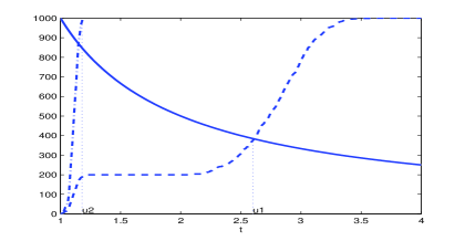
Figure 1: $X$-axis: Common size $t_{1}$. $Y-$axis: number $p$ of groups. Solid line: $g(u)=k/u$. Dashed line: $p(u)$ for $\rho=0.5,\pi=20\%$ (see simulation part). Dot dashed line: $p(u)*logp(u))$. Dot lines: corresponding $u_{1}$, $u_{2}$ positions. $n=200$, $k=1000$, $SNR=5$. We observe $u_{2}<u_{1}$.

5.4.2 Determination of the delegates

The set of ’delegates’

$${\mathcal{D}}=\left\{\ell\in\{1,\ldots,k\},\,\exists\ell^{\prime}\in\{1,\ldots,k\}\setminus\{\ell\}\mbox{ such that }|\Gamma_{\ell\ell^{\prime}}|>\gamma/p^{*}\right\}$$

is also identified with the ’task’ $t=1$. Each delegate is associated to one group. It remains to distribute the variables whose indices are not in the ${\mathcal{D}}$ in the different $p^{*}$ groups.

5.4.3 Completion of the groups

The variable of rank one in each group ${\mathcal{G}}_{j}$ is a variable belonging to $\mathcal{D}$. The repartition is done in such a way that all the groups have the same (or almost the same) cardinality. In the same way as for the gathering Grouping procedures, we propose two versions for the Boosting Grouping:

• (BGc): We rearrange the groups by sorting the correlation indicators associated to the delegates: $R_{(1)}\geq\ldots\geq R_{(p^{*})}$. This means that ${\mathcal{G}}_{1}$ contains the delegate $\ell_{1}$ such that $R_{\ell_{1}}=Y^{t}X_{.\ell_{1}}$ takes the largest correlation value (equal to $R_{(1)}$) and ${\mathcal{G}}_{p^{*}}$ has the delegate with the smallest $R_{\ell_{p^{*}}}$ correlation value (equal to $R_{(p^{*})}$). The groups are then built such that the $R$’s are as homogeneous as possible in each group and as close as possible to their delegate. Grouping starts by ranking the remaining $R$’s (i.e. not associated to a delegate): $R_{(1)}\geq\ldots\geq R_{(k-p^{*})}$. We denote $(\ell)$ the index associated to the quantity $R_{(\ell)}$. The $p^{*}$ different groups are then successively filled by using the ranking indices:

  $${\mathcal{G}}_{1}=\{\,\ell_{1},(1),\ldots,(\lfloor k/p^{*}\rfloor)-1\,\},\quad\ldots\quad,{\mathcal{G}}_{p^{*}}=\{\,\ell_{p^{*}},(k-p^{*}-\lfloor k/p^{*}\rfloor)+1),\ldots,(k-p^{*})\,\}.$$

• (BGa): It is the same procedure as (BGc) but using the $|R|$’s instead of the the $R$’s. Notice that in this case, we have rearranged the groups by sorting the absolute value of the correlation indicators associated to the delegates.

Again, to understand the improvement provided by the BGa and BGc in the next section, we also consider

• (BGr): the groups are filled up completed randomly. The $k-p^{*}$ variables are spread out randomly into the $p^{*}$ groups.

5.5 Quality of BRG

Let us now consider the estimator $\hat{\beta}^{*}$ of $\beta$ obtained using the procedure GR-LOL combined with a pre-processing using BRG algorithm to form the groups. Applying Theorem 1 under the conditions of the theorem, it is easy to show that as soon as $\gamma\geq c[\log p/n]^{1/2}$

$$E\|\hat{\beta}^{*}-\beta\|_{2}^{2} \leq C\,\left(\gamma\right)^{2-q}.$$ (21)

6 Simulation

In this section, an extensive simulation study is conducted to explore the practical qualities of procedure GR-LOL as well as the Boosting Grouping (BRG) procedure. In the first part, we briefly describe the experimental design and the empirical tuning of the parameters of the procedure. The second part is devoted to the study of the Boosting Grouping procedures comparing to the gathered procedures given in Section 5.2 and to the procedures GGr and BGr where the groups are filled randomly. Finally, GR-LOL procedure (with a pre BRG-processing) is compared with two other procedures: LOL and Group Lasso. The comparison with LOL (see Mougeot et al., (2012)) allows to check the contribution of the grouping and the comparison with the Group lasso (see Yuan and Lin, (2006)) allows to evaluate GR-LOL with respect to this challenging procedure involving an important optimization step.

6.1 Experimental design

6.1.1 Generation of the variables

The design matrix $X$ is a standard Gaussian $n\times k$ matrix. Each column vector $X_{\cdot\ell}$ is centered and normalized. The target observations $Y$ are given by $Y=X\beta+W$ where

• $\beta$ is a vector of size $k$ whose coordinates are zero except $S$ which are $\beta_{\ell}=(-1)^{b_{\ell}}|z_{\ell}|$ for $\ell=1,\ldots,S$ where the $b$’s are i.i.d. Rademacher variables and the $z$’s are i.i.d. ${\cal N}(5,1)$ variables.

• $W$ are i.i.d. variables ${\cal N}(0,\sigma^{2})$. The variance $\sigma^{2}$ of the noise is chosen such that the SNR (signal over noise ratio) is close to $5$ which corresponds to a middle noise level.

To introduce some dependency between the regressors, we choose randomly a set denoted $\mathcal{R}$ of size $p_{d}=\lfloor\pi k\rfloor$ of variables among the $k$ initial variables. Let us denote by $M_{\rho}$ the $p_{d}\times p_{d}$ correlation matrix such that $M_{\rho}(i,i)=1$ and $M_{\rho}(i,j)=\rho$ if $i\not=j$. Let $V$ the eigenvector matrix and $D$ the diagonal eigenvalue matrix of $M_{\rho}$ satisfying the singular value decomposition $M_{\rho}=VDV^{t}$. Simulating a random gaussian matrix $Z$ of size $n\times p_{d}$, we compute $X_{\mathcal{R}}=ZD^{1/2}V^{t}$; this resulting matrix has columns $X_{\ell}$ and $X_{\ell^{\prime}}$ verifying $cor(X_{\ell},X_{\ell^{\prime}})=\rho$ as soon as $\ell\neq\ell^{\prime}$. In order to study broad experiments, different proportion values ($\pi=5\%,10\%,20\%$) as correlation values ($\rho=0.0,0.6,0.8$) have been studied. This method has the advantage to tune accurately the number of correlated variables as well as the amount of correlation between the variables.

6.1.2 Tuning parameters of the algorithms

As usual for thresholding methods, parameters $\lambda_{n}(1)$ and $\lambda_{n}(2)$ involved in the GR-LOL procedure are critical values quite hard to tune because they depend on constants which are not optimized and may not be available in practice. In this work, we tune them in an empirical way described as follows:

Threshold $\lambda_{n}(1)$.

The first threshold is used to select the leader groups. Remember that at this stage, the number $p$ of groups is known, (or determined by BG). Indeed, we do not determine directly the level $\lambda_{n}(1)$ but find the number $p_{0}$ of leader groups which is equivalent. Rearrange the groups along the values of $\rho_{j}$ and denote ${\mathcal{G}}_{(1)},\ldots,{\mathcal{G}}_{(p)}$ the result of the ranking. More precisely, the group ${\mathcal{G}}_{(j)}$ is associated to the quantity $\rho_{(j)}$ where $\rho_{(j)}$ is the $j$th element of the list $\rho_{(1)}^{2}\geq\ldots\geq\rho_{(p)}^{2}$. We also denote $t_{(j)}$ the cardinality of such a group ${\mathcal{G}}_{(j)}$ and $p_{0}$ is simply determined by

$$\sum_{j=1}^{p_{0}}t_{(j)}<n\quad\mbox{ and }\quad\sum_{j=1}^{p_{0}+1}t_{(j)}\geq n.$$

When using grouping procedures, original variables are not handled directly but through groups. If an important variable (i.e. associated with a large coefficient of correlation with the target) belongs to a cluster among unimportant variables (associated with small coefficients), this variable may easily be unseen and killed during the first thresholding step. This procedure slightly differs from the LOL original procedure in being much less restrictive during the first thresholding step and allowing to finally keep more variables through the groups.

Threshold $\lambda_{n}(2)$.

In order to compute the second thresholding step, we do not determine, as previously, directly the level $\lambda_{2}(n)$ but find the number $p_{1}$ of finally retained groups which is equivalent. The second threshold $\lambda_{n}(2)$ used for denoising is computed by $5$-fold cross-validation. A proportion of $80\%$ of the observations are used to estimate the $\beta$ coefficients.

The $p_{0}$ groups, kept after the first thresholding, are ranked using the $l^{2}$-norm of their estimated coefficients, $\|\hat{\beta}\|_{{\mathcal{G}}_{j},2}$. Each ${\mathcal{G}}_{(j)}$ group, associated to the quantity $\|\hat{\beta}\|_{{\mathcal{G}}_{j},2}$ is corresponding to the $j$th element of the list $\|\hat{\beta}\|_{{\mathcal{G}}_{(}1),2}\geq\ldots\geq\|\hat{\beta}\|_{{\mathcal{G}}_{(}p_{0}),2}$. The $20\%$ remaining observations are used to sequentially compute the prediction error using the one, …, the $j$th first groups of the previous ranking list. Using a model involving the $j$th first groups, the prediction error is defined by $\|Y-\hat{Y}_{{\cal U}_{j}}\|_{2}^{2}$ where ${\cal U}_{j}={\mathcal{G}}_{(1)}\cup\ldots\cup{\mathcal{G}}_{(j)}$. The prediction error is averaged using the $5$-fold cross-validation. Finally, the first groups corresponding to the minimum prediction error are kept.

In Section 6.2, we use LOL and the Group Lasso algorithms which both tuning parameters as well. LOL algorithm is a particularly case of GR-LOL when the number of groups equals the number of variables i.e. $p=k$. For fair comparison, we use here for LOL the same algorithm as for GR-LOL in the case where $p=k$. (And so we have here a slight difference with the LOLA procedure provided in Mougeot et al., (2012).) For group Lasso, the number of final groups is computed by cross-validation as described in (Yuan and Lin, (2006), Ma et al., (2007), Huang et al., (2010)). As usual, the initial sample of observations is split into two samples: the training set contains $75\%$ of the $n$ observations and is used when the algorithms are running, the test set contains $25\%$ of the $n$ observations and is used for the cross-validation methods.

6.1.3 Criterion to evaluate the quality of the method

For each studied procedure $P$ ($P$ is either $BG_{(a,c,r)}$ or $GG_{(a,c,r)}$) with the prediction $\hat{Y}^{P}$, the relative prediction error $E_{Y}^{P}=\|Y-\hat{Y}^{P}\|_{2}^{2}/\|Y\|_{2}^{2}$ is computed on the target $Y$. The results presented in the tables give median values and standard deviations when $K=100$ replications of the algorithms are performed. When GR-LOL is compared with another procedure $P$ ($P$ is either LOL or Group Lasso), the ratio $E_{Y}^{P}/E_{Y}^{GR-LOL}$ is computed. If the ratio is close to $1$, the methods perform similarly; when the ratio is larger than $1$, GR-LOL outperforms P.

6.1.4 BRG: Number $p$ of groups

Recall that the first step of BRG consists in determining the number $p^{*}$ of groups. and is detailed in Section 5.4.1. Figure 2 shows the average size of the groups computed with the BRG procedure when the level of dependence between the regressors given by $\pi$ and $\rho$ are varying continuously. When no dependency is introduced in the design matrix, we observe that the groups contain in average $t^{*}=1.5$ variables using the experimental design previously described. Observe that the size of the groups is increasing (and then the number $p^{*}$ of groups is decreasing) with the level of dependency between the regressors (with $\pi$ or $\rho$). For example, for $\rho=0.8$, the size of the group is almost multiplied by 2 as $\pi$ decreases from $50\%$ to $10\%$.

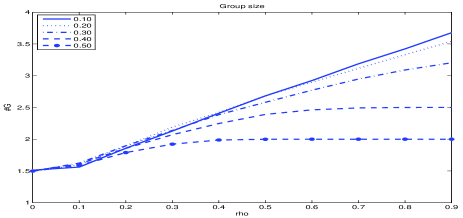
Figure 2: $Y$-axis: Size of the groups. $X-$axis: correlation $\rho$ between the regressors for $\pi=10\%,20\%,30\%,40\%,50\%$. $n=200$, $k=1000$, $SNR=5$, $K=100$.

For a fair comparison, the number $p^{*}$ of groups is the same for all the methods, only the repartition of the variables between the different groups varies. Defining the number of groups is not an easy task. It should be underlined that in this case, the Random Grouping and the Gathered Grouping both benefit of the optimal and automatic choice of $p^{*}$ proposed by the boosting strategy. It should also be noticed that the Gathered and Boosting Grouping algorithms provide very different configurations for the groups, as the average size $t^{*}$ of the groups is small.

6.1.5 Impact on the Coherence

The empirical coherence $\gamma_{BG}$, $\gamma_{BT}$ and $\gamma$ are computed and shown in Table 1 for different value of correlation ($\pi=0\%,20\%,40\%$ ; $\rho=0.0,0.6,0.8$) and for all the considered grouping strategies. For each simulation, we have $\gamma=$sup$(\gamma_{BT},\gamma_{BG})$. As the results presented in table 1 are averaged over $K=100$ replications, we do not find necessarily at the end this property, especially for Gathering grouping (GGa, GGc, GGr) which can provide very different groups each time.

As expected, the boosting strategies induce a strong decrease of $\gamma_{BT}$ as soon as there exists some dependency ($\pi>20\%$, $\rho>0.6$). The different strategies for filling the groups (BGr, BGc, BGa) does not have however any influence on $\gamma_{BG}$ as expected also. The gathered groupings (GGc, GGa) do not help to reduce $\gamma_{BT}$ and $\tau^{*}$. As expected, the empirical coherence (denoted $\gamma$ in the theoretical part) is increasing with the dependence level $\rho$. Table 1 shows also the empirical value of $\tau^{*}=t^{*}\gamma_{BT}+\gamma_{BG}$ and $r^{*}=t^{*}\gamma_{BT}^{2}+\gamma_{BG}^{2}$ computed for different strategies.

$\pi=0\%$, $\rho=0.0$	$t^{*}$	$\gamma_{BT}$	$\gamma_{BG}$	$\gamma$	$\tau^{*}$	$r^{*}$
GGr	1.40 (0.06)	0.321 (0.030)	0.317 (0.014)	0.327 (0.015)	0.766	0.245
GGc	1.40 (0.06)	0.318 (0.029)	0.321 (0.016)	0.327 (0.015)	0.766	0.245
GGa	1.40 (0.06)	0.318 (0.029)	0.319 (0.017)	0.327 (0.015)	0.764	0.243
BGr	1.40 (0.06)	0.234 (0.016)	0.327 (0.015)	0.327 (0.015)	0.655	0.184
BGc	1.40 (0.06)	0.234 (0.015)	0.327 (0.015)	0.327 (0.015)	0.655	0.184
BGa	1.40 (0.06)	0.234 (0.015)	0.327 (0.015)	0.327 (0.015)	0.655	0.184
$\pi=20\%$, $\rho=0.6$	$t^{*}$	$\gamma_{BT}$	$\gamma_{BG}$	$\gamma$	$\tau$	$\tau^{*}$
GGr	2.80 (0.07)	0.731 (0.029)	0.723 (0.020)	0.733 (0.018)	2.770	2.019
GGc	2.80 (0.07)	0.730 (0.032)	0.726 (0.019)	0.733 (0.018)	2.770	2.019
GGa	2.80 (0.07)	0.730 (0.032)	0.724 (0.019)	0.733 (0.018)	2.768	2.016
BGr	2.80 (0.07)	0.260 (0.018)	0.733 (0.018)	0.733 (0.018)	1.460	0.726
BGc	2.80 (0.07)	0.260 (0.016)	0.733 (0.018)	0.733 (0.018)	1.460	0.726
BGa	2.80 (0.07)	0.260 (0.016)	0.733 (0.018)	0.733 (0.018)	1.460	0.726
$\pi=40\%$, $\rho=0.6$	$t^{*}$	$\gamma_{BT}$	$\gamma_{BG}$	$\gamma$	$\tau$	$\tau^{*}$
GGr	2.40 (0.02)	0.742 (0.030)	0.739 (0.019)	0.746 (0.019)	2.521	1.869
GGc	2.40 (0.02)	0.742 (0.031)	0.740 (0.019)	0.746 (0.019)	2.522	1.870
GGa	2.40 (0.02)	0.741 (0.031)	0.740 (0.019)	0.746 (0.019)	2.519	1.866
BGr	2.40 (0.02)	0.303 (0.024)	0.746 (0.019)	0.746 (0.019)	1.474	0.778
BGc	2.40 (0.02)	0.303 (0.024)	0.746 (0.019)	0.746 (0.019)	1.474	0.778
BGa	2.40 (0.02)	0.303 (0.021)	0.746 (0.019)	0.746 (0.019)	1.473	0.777
$\pi=40\%$, $\rho=0.8$	$t^{*}$	$\gamma_{BT}$	$\gamma_{BG}$	$\gamma$	$\tau$	$\tau^{*}$
GGr	2.50 (0.03)	0.868 (0.016)	0.866 (0.011)	0.869 (0.011)	3.035	2.631
GGc	2.50 (0.03)	0.867 (0.017)	0.867 (0.011)	0.869 (0.011)	3.035	2.632
GGa	2.50 (0.03)	0.867 (0.017)	0.867 (0.011)	0.869 (0.011)	3.035	2.632
BGr	2.50 (0.03)	0.315 (0.025)	0.869 (0.010)	0.869 (0.010)	1.656	1.003
BGc	2.50 (0.03)	0.314 (0.028)	0.869 (0.010)	0.869 (0.010)	1.654	1.002
BGa	2.50 (0.03)	0.317 (0.025)	0.869 (0.010)	0.869 (0.010)	1.662	1.007

Table 1: First line: Empirical coherence $\gamma_{BG}$, $\gamma_{BT}$, $\gamma$ computed when the groups are built using the different strategies. $SNR=5$, $n=200$, $k=1000$, $K=100$, $\pi=40\%$.

6.1.6 Benefits of boosting grouping

Table 2 compares the random (GGr), Gathered (GGc, GGa) and boosting grouping (BGr, BGc, BGa) for different sparsities $S$ and different levels of dependence ($\rho,\pi)$.

$\pi=0\%,\rho=0$	$S=10$	$S=20$	$S=30$	$S=40$	$S=50$
GGr	3.06 ( 0.02)	6.32 ( 0.04)	11.36 ( 0.07)	14.11 ( 0.09)	14.53 ( 0.10)
GGc	3.18 ( 0.02)	5.18 ( 0.03)	7.86 ( 0.04)	9.81 ( 0.08)	10.36 ( 0.06)
GGa	2.97 ( 0.02)	4.93 ( 0.02)	7.62 ( 0.04)	9.19 ( 0.07)	10.31 ( 0.06)
BGr	3.09 ( 0.02)	7.09 ( 0.04)	10.62 ( 0.06)	11.64 ( 0.07)	14.21 ( 0.09)
BGc	3.15 ( 0.02)	5.71 ( 0.05)	9.84 ( 0.06)	12.30 ( 0.07)	12.31 ( 0.07)
BGa	3.04 ( 0.02)	5.33 ( 0.03)	8.32 ( 0.05)	10.12 ( 0.06)	10.97 ( 0.07)
$\pi=20\%,\rho=0.6$	$S=10$	$S=20$	$S=30$	$S=40$	$S=50$
GGr	8.85 ( 0.16)	28.82 ( 0.22)	36.43 ( 0.23)	40.61 ( 0.24)	44.56 ( 0.23)
GGc	7.52 ( 0.18)	21.61 ( 0.24)	41.72 ( 0.26)	38.04 ( 0.26)	37.50 ( 0.24)
GGa	7.93 ( 0.17)	24.43 ( 0.24)	33.26 ( 0.26)	40.67 ( 0.27)	39.98 ( 0.24)
BGr	9.35 ( 0.13)	20.28 ( 0.17)	25.35 ( 0.19)	35.28 ( 0.20)	32.80 ( 0.17)
BGc	7.22 ( 0.10)	14.41 ( 0.15)	24.76 ( 0.16)	25.50 ( 0.18)	27.43 ( 0.19)
BGa	6.04 ( 0.05)	10.02 ( 0.06)	14.14 ( 0.10)	20.96 ( 0.13)	20.35 ( 0.14)
$\pi=40\%,\rho=0.6$	$S=10$	$S=20$	$S=30$	$S=40$	$S=50$
GGr	19.78 ( 0.19)	31.66 ( 0.20)	39.23 ( 0.21)	45.73 ( 0.22)	44.66 ( 0.21)
GGc	17.74 ( 0.18)	38.77 ( 0.22)	38.96 ( 0.23)	51.72 ( 0.22)	51.14 ( 0.23)
GGa	18.28 ( 0.19)	40.82 ( 0.22)	43.42 ( 0.21)	59.12 ( 0.22)	54.80 ( 0.23)
BGr	10.51 ( 0.07)	17.34 ( 0.11)	24.71 ( 0.13)	30.16 ( 0.16)	31.15 ( 0.19)
BGc	9.48 ( 0.09)	19.03 ( 0.14)	24.26 ( 0.16)	30.14 ( 0.17)	31.27 ( 0.18)
BGa	7.51 ( 0.06)	10.43 ( 0.07)	16.30 ( 0.09)	20.63 ( 0.12)	23.41 (0.13)
$\pi=40\%,\rho=0.8$	$S=10$	$S=20$	$S=30$	$S=40$	$S=50$
GGr	29.75 ( 0.20)	43.95 ( 0.23)	39.27 ( 0.23)	48.75 ( 0.22)	48.80 ( 0.27)
GGc	37.59 ( 0.22)	49.77 ( 0.25)	49.81 ( 0.26)	57.23 ( 0.24)	53.57 ( 0.26)
GGa	36.69 ( 0.21)	51.53 ( 0.25)	50.64 ( 0.26)	59.99 ( 0.25)	60.64 ( 0.26)
BGr	7.85 ( 0.05)	13.95 ( 0.08)	18.14 ( 0.13)	19.82 ( 0.17)	26.48 ( 0.19)
BGc	8.33 ( 0.07)	14.93 ( 0.11)	20.52 ( 0.15)	21.41 ( 0.17)	28.95 ( 0.18)
BGa	5.96 ( 0.05)	9.19 ( 0.05)	12.72 ( 0.10)	16.26 ( 0.13)	19.44 ( 0.17)

Table 2: Relative prediction errors $E_{Y}$ ($\times 100$) for Boosting Grouping (BGr, BGc, BGa), Gathered Grouping (GGc, GGa) and Random Grouping (GGr) when the sparsity is varying, for various levels of dependency given by $\pi,\rho$. $SNR=5$, $n=200$, $k=1000$, $K=100$.

Let us first comment the no-dependency case ($\pi=0$). When the sparsity is high ($S=10,20,30$), similar performances are obtained for any grouping strategy. Underline that even building the groups in a completely random manner is not a bad strategy. When the sparsity is low ($S=40,50$), the Gathered Groupings (GGa and GGc) bring the best results with a weak variability (low standard deviation). As there is no specific correlation between the regressors, the boosting procedure brings as expected in this case no added value.

Actually, the boosting grouping procedure is especially adapted to large correlation for taking advantage. For instance, when $\rho$ and $\pi$ are significative ($\rho=0.6$ and $\pi=0.4$), the boosting procedure clearly shows substantial benefits. However, the performances of the boosting depends on the strategy for filling the groups. When the number of correlated variables is weak ($\pi=0.2$), the boosting associated with groups filled randomly (BGr) is rather competitive compared to Gathered groupings (GGc, GGa). However, the boosting procedures with groups filled homogeneously always show the best performances (BGc, BGa) with a preference for the absolute value criteria. When there are strong correlations between the regressors $\rho=0.6,0.8$, the boosting procedures (BRc, BGa) clearly outperforms the random and the Gathered grouping, and this is even true when the groups are filled randomly (BGR). BGa always brings the best results when the sparsity $S$ increases and/or the correlation $\rho$ between the regressors increases.

6.2 Study of the GR-LOL procedure

In this part, we present the performance results when GR-LOL procedure associated with the Boosting Grouping strategy (BGa) is applied on the experimental design presented above. Comparisons between GR-LOL and LOL on the one hand, and GR-LOL and Group-lasso on the second hand are explored.

6.2.1 GR-LOL versus LOL

The main difference between LOL and GR-LOL is that GR-LOL manipulates groups of variables while LOL procedure handles the variables directly. Table 3 shows a comparison of the performances obtained for LOL for the same experimental design as above.

$\pi$	$\rho$	$S=10$	$S=20$	$S=30$	$S=40$	$S=50$
$0\%$	0.00	1.083	1.522	1.616	1.777	1.666
$20\%$	0.60	1.342	2.854	3.572	2.636	2.414
$20\%$	0.80	1.877	5.436	3.898	3.117	2.649
$40\%$	0.60	3.607	4.341	3.715	2.856	2.410
$40\%$	0.80	6.287	6.429	4.773	3.440	3.417

Table 3: Relative prediction errors ratio $E_{Y}^{LOL}/E_{Y}^{GR-LOL}$ for LOL and GR-LOL when the sparsity is varying for different correlation values $\rho=0.0,0.6,0.8$ and rates $\pi=0,0.2,0.4$. $SNR=5$, $n=200$, $k=1000$.

We observe that LOL procedure performs particularly well when the sparsity is large ($S$ small) and when the dependence between the regressors is weak (Mougeot et al., (2012)). In this case, GR-LOL brings no improvement compared to LOL. Observe that, if there is no dependency (case where $\rho=0.0$), the grouping improves the performances of LOL when the sparsity decreases ($S$ increases). If the dependency increases (case where $\rho=0.6,0.8$), GR-LOL always outperforms LOL for any considered sparsity.

6.2.2 GR-LOL versus Group-lasso

The group Lasso is one of the most popular procedure for penalized regression with grouping variables so we choose this method to challenge the boosting Grouping procedure. To be fair, for both procedures, the groups are built using the boosting strategy (BGa) and cross-validation are both used to determine the final model.

Comparison of prediction results are given by Table 4. Both procedures show similar behaviors in two cases: when there is no high correlation between the co variables ($\pi=0$) or when the sparsity ($S=50$) is small. In the other cases (especially when the sparsity is large i.e. $S$ small), the results given by GR-LOL are excellent: GR-LOL always outperforms the group lasso.

$\pi$	$\rho$	$S=10$	$S=20$	$S=30$	$S=40$	$S=50$
$0\%$	0.0	1.228	1.318	1.143	1.827	2.001
$5\%$	0.6	4.584	2.366	1.470	1.944	1.706
$5\%$	0.8	5.179	2.490	1.937	1.122	0.829
$10\%$	0.6	2.764	3.124	1.892	1.825	0.967
$10\%$	0.8	4.744	1.643	1.824	1.511	0.739
$20\%$	0.6	2.176	3.032	1.764	1.385	1.426
$20\%$	0.8	3.250	3.015	1.986	1.098	1.048

Table 4: Relative prediction errors ratio $E_{Y}^{GLasso}/E_{Y}^{GR-LOL}$ for GR-LOL and GLasso when the sparsity is varying, for various levels of dependency given by $\pi,\rho$. $SNR=5$, $n=200$, $k=1000$.

To end this comparison, let us give a few words about computational aspects. The Group Lasso algorithm is based on an optimization procedure which can be time consuming while GR-LOL procedure solves the penalized regression using two thresholding steps and a classical regression. Regarding the complexity of the different methods, GR-LOL has a strong advantage over the Group Lasso.

6.3 Conclusion

This experimental study shows that true benefits can be obtained using a grouping approach for penalized regression even in the case where there is no prior knowledge on the groups. However, the results are highly relying on the grouping strategy. The boosting strategy brings a nice answer to the grouping problem when no prior information is available on the structured sparsity. This strategy is very easy to implement and especially well adapted when a strong correlation exists between the regressors in the case of high sparsity ($S$ small).

7 Proofs

7.1 RIP and associated properties: $\tau^{*}$-conditions

In this part, we collect properties which are linked with the coherence $\tau^{*}$. All these inequalities are extensively used in the proof of Theorem 1 and the proofs of the propositions stated in Section 7.2; their proofs are detailed in the appendix.

Recall that for $\mathcal{I}\subset\{1,\ldots,k\}$, $\Gamma_{\mathcal{I}}=\widetilde{X}_{\mathcal{I}}^{t}\widetilde{X}_{\mathcal{I}}$ is the associated Gram matrix of $\widetilde{X}_{\mathcal{I}}$. $\widetilde{X}_{\mathcal{I}}$ is the matrix restricted to the columns of $\widetilde{X}$ whose indices are in $\mathcal{I}$. Denote by $P_{V_{\mathcal{I}}}$ the projection on the space ${V_{\mathcal{I}}}$ spanned by the predictors $\widetilde{X}_{\ell}$ whose indices $\ell$ belong to $\mathcal{I}$. We also denote $\bar{\alpha}(\mathcal{I})$ the vector of $\mathbb{R}^{\#(\mathcal{I})}$, such that

$$\widetilde{X}_{\mathcal{I}}\bar{\alpha}(\mathcal{I})=P_{V_{\mathcal{I}}}[\widetilde{X}\alpha].$$ (22)

As well, we define $\hat{\alpha}(\mathcal{I})$ the vector of $\mathbb{R}^{\#(\mathcal{I})}$, such that

$$\widetilde{X}_{\mathcal{I}}\hat{\alpha}(\mathcal{I})=P_{V_{\mathcal{I}}}[Y].$$ (23)

The following lemma describes the ’bloc-diagonal’ aspect of the Gram matrices $\Gamma_{\mathcal{I}}$ at least when the set of indices $\mathcal{I}$ is small enough. It is corresponding to the ’group-version’ of the link between coherence and RIP property (see for instance the corresponding result in Mougeot et al., (2012)).

Lemma 1.

(RIP-property) Let $0<\nu<1$ be fixed. Let $\mathcal{I}$ be a subset of $\{1,\ldots,k\}$ such that $\tau(\mathcal{I})\leq\nu$. Then we get

$$\forall x\in\mathbb{R}^{\#(\mathcal{I})},\quad\ \|x\|_{2}^{2}(1-\nu)\leq x^{t}\,\Gamma_{\mathcal{I}}\,x\leq\|x\|_{2}^{2}(1+\nu).$$ (24)

We deduce that the Gram matrix $\Gamma_{\mathcal{I}}$ is almost diagonal and in particular invertible as soon as $\tau(\mathcal{I})\leq\nu$. When this upper bound on $\tau(\mathcal{I})$ holds, we also extensively use the RIP Property (24) in the following forms:

$$\forall x\in\mathbb{R}^{\#(\mathcal{I})},\;\|x\|_{2}^{2}(1+\nu)^{-1}\leq x^{t}\,\Gamma_{\mathcal{I}}^{-1}\,x\leq(1-\nu)^{-1}\|x\|_{2}^{2}\,,$$ (25)

and

$$\forall x\in\mathbb{R}^{\#(\mathcal{I})},\;(1-\nu)\|x\|_{2}^{2}\leq\|\sum_{\ell\in\mathcal{I}}x_{\ell}\;\widetilde{X}_{\bullet\ell}\;\|_{2}^{2}\leq(1+\nu)\|x\|_{2}^{2}\,.$$ (26)

We also need the following lemma

Lemma 2.

For any $\mathcal{I}$ subset of $\{1,\ldots,k\}$ such that $\tau(\mathcal{I})\leq\nu$, we have

$$\forall x\in\mathbb{R}^{n},\;(1+\nu)^{-1}\sum_{\ell\,\in\mathcal{I}}\;\left(\sum_{i=1}^{n}x_{i}\widetilde{X}_{i,\ell}\right)^{2}\leq\|P_{V_{\mathcal{I}}}x\|_{2}^{2}\leq(1-\nu)^{-1}\sum_{\ell\,\in\mathcal{I}}\;\left(\sum_{i=1}^{n}x_{i}\widetilde{X}_{i,\ell}\right)^{2}\,.$$ (27)

7.2 Behavior of the projectors: $r^{*}$-conditions

In this subsection, we describe properties of the projection which are more general as in the previous part where the results were linked to the RIP property. These properties depend on the index $r^{*}=t^{*}\;\gamma_{BT}^{2}+\gamma_{BG}^{2}$. It is noteworthy to observe that in the no-group setting, we do not need to introduce this indicator $r^{*}$ since in this case $r^{*}=(\tau^{*})^{2}$. Hence this is one of the precise place where the grouping induces different argument.

Let now state the following different technical results, which are essential in the sequel.

Lemma 3.

Let $\mathcal{I},{\mathcal{C}}$ be subsets of $\{1,\ldots,k\}$ and put

$$B({\mathcal{C}})_{\ell}=\sum_{\ell^{\prime}\in{\mathcal{C}},\ell^{\prime}\not=\ell}\;\Gamma_{\ell\ell^{\prime}}{\alpha}_{\ell^{\prime}}$$

for any $\ell$. Then, we have

$$\|B({\mathcal{C}})\|_{\mathcal{I},2}^{2} \leq\;2\;\|\alpha\|_{{\mathcal{C}},1}^{2}\,r(\mathcal{I})$$

where $r(\mathcal{I})$ is defined in (LABEL:rI).

Proposition 1.

For any integer $j$ from $\{1,\ldots,p\}$, we get

$$\left|\,\|R\|_{{\mathcal{G}}_{j},2}-\|\alpha\|_{{\mathcal{G}}_{j},2}\right|^{2}\leq 4M^{2}v_{n}r({\mathcal{G}}_{j})+2(1+\nu)\|P_{V_{{\mathcal{G}}_{j}}}W\|_{2}^{2}.$$

Proposition 2.

For any subset $\mathcal{I}$ of the leaders indices set ${\mathcal{G}}_{\mathcal{B}}$, there exists $\kappa$ depending on $\nu$ such that

$$\|\widehat{\alpha}-{\alpha}\|_{\mathcal{I},2}^{2}\;{\mathbb{I}}\{\mathcal{I}\subset{\mathcal{G}}_{\mathcal{B}}\} \leq\kappa\,\left(\|\alpha\|_{1}^{2}\,r(\mathcal{I})+\|P_{V_{\mathcal{I}}}W\|_{2}^{2}+\,\|P_{V_{{\mathcal{G}}_{\mathcal{B}}}}W\|_{2}^{2}\,r(\mathcal{I})\right).$$

More precisely

$$\kappa\geq\frac{1}{1-\nu}\vee\frac{6}{(1-\nu)^{3}}\vee\frac{4(2\nu^{2}-\nu+2)}{(1-\nu)^{4}}.$$

Proposition 3.

Let $\mathcal{I}$ be a non random subset such that $\#(\mathcal{I})\leq n_{\mathcal{I}}$, where $n_{\mathcal{I}}$ is a deterministic quantity, then

$$P\left(\frac{1}{\sigma^{2}}\|P_{V_{\mathcal{I}}}[W]\|_{2}^{2}\geq z^{2}\right) \leq\exp\left(-z^{2}/16\right)$$ (28)

for any $z$ such that $z^{2}\geq 4\,n_{\mathcal{I}}$. If now $\mathcal{I}$ is a random subset of the form $\{(j,t),\;j\in A,\;1\leq t\leq t_{j}\}$ where $A$ is a random set of $\{1,\ldots,p\}$ of cardinal less than $L$ (deterministic constant), Inequality (28) is still true but for any $z$ such that $z^{2}\geq 16\,L\,(t^{*}\vee\log{p})$. In particular, this implies that for such a set, for any $k\geq 1$, there exists a constant $C_{k}$ such that

$$E\left(\,\frac{1}{\sigma^{2}}\|P_{V_{\mathcal{I}}}[W]\|_{2}^{2}\,\right)^{k}\leq C_{k}L^{k}\,\left(t^{*}\vee\log{p}\right)^{k}.$$ (29)

7.3 Proof of the Theorem

Thanks to Condition (3), we have

$$a\nu_{n}\;\|\hat{\beta}^{*}-\beta\|_{2}^{2}\leq\|\hat{\alpha}^{*}-\alpha\|_{2}^{2}\leq b\nu_{n}\;\|\hat{\beta}^{*}-\beta\|_{2}^{2}$$

which allows us to focus on the estimation error $\|\hat{\alpha}^{*}-\alpha\|_{2}$. We have

$$\|\hat{\alpha}^{*}-\alpha\|_{2}^{2} =\|\hat{\alpha}^{*}-\alpha\|_{{\mathcal{G}}_{\mathcal{B}},2}^{2}+\|\alpha\|_{({\mathcal{G}}_{\mathcal{B}})^{c},2}^{2}:=I\;(\mbox{In})\;+O\;(\mbox{Out}).$$

We split $I$ into four terms :

$$I =\sum_{j\in{\mathcal{B}}}{\mathbb{I}}\{\|\hat{\alpha}\|_{{\mathcal{G}}_{j},2}\geq\lambda_{n}(2)\}\;{\mathbb{I}}\{\|{\alpha}\|_{{\mathcal{G}}_{j},2}\geq\lambda_{n}(2)/2\}\;\|\hat{\alpha}-\alpha\|_{{\mathcal{G}}_{j},2}^{2}$$

$$+\sum_{j\in{\mathcal{B}}}{\mathbb{I}}\{\|\hat{\alpha}\|_{{\mathcal{G}}_{j},2}\geq\lambda_{n}(2)\}\;{\mathbb{I}}\{\|{\alpha}\|_{{\mathcal{G}}_{j},2}<\lambda_{n}(2)/2\}\;\|\hat{\alpha}-\alpha\|_{{\mathcal{G}}_{j},2}^{2}$$

$$+\sum_{j\in{\mathcal{B}}}{\mathbb{I}}\{\|\hat{\alpha}\|_{{\mathcal{G}}_{j},2}<\lambda_{n}(2)\}\;{\mathbb{I}}\{\|\alpha\|_{{\mathcal{G}}_{j},2}\geq 2\lambda_{n}(2)\}\;\|\alpha\|_{{\mathcal{G}}_{j},2}^{2}$$

$$+\sum_{j\in{\mathcal{B}}}{\mathbb{I}}\{\|\hat{\alpha}(\|_{{\mathcal{G}}_{j},2}<\lambda_{n}(2)\}\;{\mathbb{I}}\{\|\alpha\|_{{\mathcal{G}}_{j},2}<2\lambda_{n}(2)\}\;\|\alpha\|_{{\mathcal{G}}_{j},2}^{2}$$

$$:=IBB\;(\mbox{InBigBig})\;+\;IBS\;(\mbox{InBigSmall})\;+ISB\;(\mbox{InSmallBig})\;+ISS\;(\mbox{InSmallSmall})\;.$$

We have on the other hand,

$$O \leq\sum_{j\in{\mathcal{B}}^{c}}{\mathbb{I}}\{\|R\|_{{\mathcal{G}}_{j},2}\leq\lambda_{n}(1)\}\;{\mathbb{I}}\{\|\alpha\|_{{\mathcal{G}}_{j},2}\geq 2\lambda_{n}(1)\}\;\|\alpha\|_{{\mathcal{G}}_{j},2}^{2}$$

$$+\sum_{j\in{\mathcal{B}}^{c}}{\mathbb{I}}\{\|R\|_{{\mathcal{G}}_{j},2}\leq\lambda_{n}(1)\}\;{\mathbb{I}}\{\|\alpha\|_{{\mathcal{G}}_{j},2}<2\lambda_{n}(1)\}\;\|\alpha\|_{{\mathcal{G}}_{j},2}^{2}$$

$$+\sum_{j\in{\mathcal{B}}^{c}}{\mathbb{I}}\{\|R\|_{{\mathcal{G}}_{j},2}\geq\lambda_{n}(1)\}\;{\mathbb{I}}\{\|\alpha\|_{{\mathcal{G}}_{j},2}\geq\lambda_{n}(1)/2\}\;\|\alpha\|_{{\mathcal{G}}_{j},2}^{2}$$

$$+\sum_{j\in{\mathcal{B}}^{c}}{\mathbb{I}}\{\|R\|_{{\mathcal{G}}_{j},2}\geq\lambda_{n}(1)\}\;{\mathbb{I}}\{\|\alpha\|_{{\mathcal{G}}_{j},2}<\lambda_{n}(1)/2\}\;\|\alpha\|_{{\mathcal{G}}_{j},2}^{2}$$

$$:=OSB\;(\mbox{OutSmallBig})\;+OSS\;(\mbox{OutSmallSmall})\;+OBB\;(\mbox{OutBigBig})\;+OBS\;(\mbox{OutBigSmall})\;.$$

7.3.1 Study of $IBB$ and $ISB$

Let us first study $ISB$. Observe that the two conditions $\|\hat{\alpha}\|_{{\mathcal{G}}_{j},2}\leq\lambda_{n}(2)$ and $\|\alpha\|_{{\mathcal{G}}_{j},2}\geq 2\lambda_{n}(2)$ imply $\|\hat{\alpha}\|_{{\mathcal{G}}_{j},2}\leq\|\alpha\|_{{\mathcal{G}}_{j},2}/2$. We deduce that

$$\|\hat{\alpha}-\alpha\|_{{\mathcal{G}}_{j},2}\geq\|\alpha\|_{{\mathcal{G}}_{j},2}-\|\hat{\alpha}\|_{{\mathcal{G}}_{j},2}\geq\|\alpha\|_{{\mathcal{G}}_{j},2}/2$$

and then

$$ISB \leq 4\,\sum_{j\in{\mathcal{B}}}{\mathbb{I}}\{\|\alpha\|_{{\mathcal{G}}_{j},2}\geq 2\lambda_{n}(2)\}\;\|\hat{\alpha}-\alpha\|_{{\mathcal{G}}_{j},2}^{2}=4\;\|\hat{\alpha}-\alpha\|_{\mathcal{I}\cap{\mathcal{G}}_{\mathcal{B}},2}^{2}$$ (30)

where

$$\mathcal{I}:=\{(j,t)\in\{1,\ldots,k\},\;\|\alpha\|_{{\mathcal{G}}_{j},2}\geq 2\lambda_{n}(2)\}.$$

Thanks to Condition 12, we get

$$n_{G}(\mathcal{I}):=\#(\,\{j,\;\exists t,\;(j,t)\in\mathcal{I}\}\,) \leq\sum_{j=1}^{p}{\mathbb{I}}\{j\in{\mathcal{C}}\},\;\left((2\lambda_{n}(2))^{-1}\|\alpha\|_{{\mathcal{G}}_{j},2}\right)^{q}\leq(2\lambda_{n}(2))^{-q}\,M^{q}\,\nu_{n}^{q/2}$$

and we bound $\#(\mathcal{I})$ by $t^{*}\times\#(\{j,\;\exists t,\;(j,t)\in\mathcal{I}\})$. It follows that

$$r(\mathcal{I}) \leq M^{q}\,v_{n}^{q/2}\,(2\lambda_{n}(2))^{-q}\,[\gamma_{BG}^{2}+t^{*}\gamma_{BT}^{2}]$$

$$\leq M^{q}\,v_{n}^{q/2}\,(2\lambda_{n}(2))^{-q}\,r^{*}.$$

Using successively Proposition 2 and Proposition 3, we get

$$E(ISB) \leq 4\kappa E\left(M^{2}v_{n}r(\mathcal{I})+\|P_{V_{\mathcal{I}}}[W]\|_{2}^{2}+r(\mathcal{I})\|P_{V_{{\mathcal{G}}_{\mathcal{B}}}}[W]\|_{2}^{2}\right)$$

$$\leq 4\kappa\left([M^{2}v_{n}r(\mathcal{I})+C_{1}\sigma^{2}[t^{*}\vee\log p][n_{G}(\mathcal{I})+r(\mathcal{I})N^{*}]\right)$$

$$\leq[4+2C_{1}]\kappa\left(M^{q}\,v_{n}^{q/2}\,(2\lambda_{n}(2))^{-q}\right)\;(\lambda^{*})^{2}$$

where $\lambda^{*}$ is defined in (19) and because $r^{*}N^{*}\leq\tau^{*}N^{*}\leq\nu$. The bound given in (30) is valid for $IBB$ and then the proof also holds for $IBB$.

7.3.2 Study of $OSS$, $OBS$ and $ISS$

Let $q$ be such that Condition (12) is satisfied

$$OSS \leq\sum_{j=1}^{p}{\mathbb{I}}\{\|\alpha\|_{{\mathcal{G}}_{j},2}<2\lambda_{n}(1)\}\;\|\alpha\|_{{\mathcal{G}}_{j},2}^{2-q+q}\leq(2\lambda_{n}(1))^{2-q}\sum_{j=1}^{p}\;\|\alpha\|_{{\mathcal{G}}_{j},1}^{q}$$

$$\leq M^{q}v_{n}^{q/2}(2\lambda_{n}(1))^{2-q}$$

Note that this proof can also be performed for $OBS$ and $ISS$ since $\lambda_{n}(1)>\lambda_{n}(2)$.

7.3.3 Study of $OSB$

Since

$$\|\alpha\|_{{\mathcal{G}}_{j},2}=\left(\|\alpha\|_{{\mathcal{G}}_{j},2}-\|R\|_{{\mathcal{G}}_{j},2}\right)+\|R\|_{{\mathcal{G}}_{j},2}$$

we get

$$OSB \leq 2\sum_{j\in{\mathcal{B}}^{c}}{\mathbb{I}}\{\|\alpha\|_{{\mathcal{G}}_{j},2}-\|R\|_{{\mathcal{G}}_{j},2}>\lambda_{n}(1)\}\;\;\left(\|\alpha\|_{{\mathcal{G}}_{j},2}-\|R\|_{{\mathcal{G}}_{j},2}\right)^{2}$$

$$+2\sum_{j\in{\mathcal{B}}^{c}}{\mathbb{I}}\{\|\alpha\|_{{\mathcal{G}}_{j},2}-\|R\|_{{\mathcal{G}}_{j},2}>\lambda_{n}(1)\}\;{\mathbb{I}}\{\|R\|_{{\mathcal{G}}_{j},2}\leq\lambda_{n}(1)\}\;\|R\|_{{\mathcal{G}}_{j},2}^{2},$$

and by Cauchy-Schwarz

$$E(OSB) \leq 2\sum_{j\leq p}\left[P\left(\,\left|\|\alpha\|_{{\mathcal{G}}_{j},2}-\|R\|_{{\mathcal{G}}_{j},2}\right|>\lambda_{n}(1)\right)\;\;E\left(\|\alpha\|_{{\mathcal{G}}_{j},2}-\|R\|_{{\mathcal{G}}_{j},2}\right)^{4}\right]^{1/2}$$

$$+2\lambda_{n}(1)^{2}\sum_{j\leq p}P\left(\,\left|\|\alpha\|_{{\mathcal{G}}_{j},2}-\|R\|_{{\mathcal{G}}_{j},2}\right|>\lambda_{n}(1)\right).$$

On the one hand, as an immediate consequence of Propositions 1 and 3, we get

$$E\left(\;\,\|R\|_{{\mathcal{G}}_{j},2}-\|\alpha\|_{{\mathcal{G}}_{j},2}\right)^{4} \leq 32M^{4}v_{n}^{2}\tau({\mathcal{G}}_{j})^{2}+16\sigma^{4}(1+\nu)^{2}\#({\mathcal{G}}_{j})^{2}.$$

Since $\#({\mathcal{G}}_{j})\leq t^{*}$ and $\tau({\mathcal{G}}_{j})\leq\tau^{*}$, we bound this term by $32(\lambda^{*})^{4}$. On the other hand, using Proposition 3,

$$P\left(\;\left|\,\|R\|_{{\mathcal{G}}_{j},2}|-\|\alpha\|_{{\mathcal{G}}_{j},2}\,\right|\geq\lambda\right) \leq P\left(\|P_{V_{{\mathcal{G}}_{j}}}W\|_{2}\geq\lambda/2(1+\nu)^{1/2}\right)$$

$$\leq\exp\left(-\lambda^{2}/32(1+\nu)\right)$$

as soon as

$$\lambda^{2}\geq\left(8M^{2}v_{n}\,r({\mathcal{G}}_{j})\right)\vee\left(16(1+\nu)\,[t^{*}\vee\log p]\right).$$

This condition is verified by $\lambda_{n}(1)$ as soon as

$$\lambda_{n}(1)\geq 4\lambda^{*}$$ (31)

and it follows

$$E(OSB) \leq\frac{9}{4}\;p\lambda_{n}(1)^{2}\;\exp\left(-\frac{\lambda_{n}(1)^{2}}{64(1+\nu)}\right).$$

7.3.4 Study of $OBB$

Let us decompose again this term into 2 different ones,

$$OBB=\sum_{j\in{\mathcal{C}}_{1}}\|\alpha\|^{2}_{{\mathcal{G}}_{j},2}+\sum_{j\in{\mathcal{C}}_{2}}\|\alpha\|^{2}_{{\mathcal{G}}_{j},2}:=OBB_{1}+OBB_{2}$$

where

$${\mathcal{C}}=\{j\in{\mathcal{B}}^{c},\;\|\alpha\|_{{\mathcal{G}}_{j},2}\geq 2\lambda_{n}(1),\,\|R\|_{{\mathcal{G}}_{j},2}\geq\lambda_{n}(1)\}$$

and

$${\mathcal{C}}_{1}={\mathcal{C}}\cap\{j,\|R\|_{{\mathcal{G}}_{j},2}\leq\|\alpha\|_{{\mathcal{G}}_{j},2}/2\}\quad\mbox{ and }\quad{\mathcal{C}}_{2}={\mathcal{C}}\cap\{j,\|R\|_{{\mathcal{G}}_{j},2}\geq\|\alpha\|_{{\mathcal{G}}_{j},2}/2\}$$

On the one hand, we obviously have

$${\mathcal{C}}_{1} \subset\{j\in\{1,\ldots,p\},\;\lambda_{n}(1)\leq\|\alpha\|_{{\mathcal{G}}_{j},2}-\|R\|_{{\mathcal{G}}_{j},2}\}$$

leading to

$$OBB_{1} \leq\sum_{j=1}^{p}{\mathbb{I}}\{\left|\,\|\alpha\|_{{\mathcal{G}}_{j},2}-\|R\|_{{\mathcal{G}}_{j},2}\right|\geq\lambda_{n}(1)\}\;\|\alpha\|^{2}_{{\mathcal{G}}_{j},2}.$$

We conclude as for the term $OSB$. For $OBB_{1}$ the argument is slightly more subtle: on the other hand,

$$j\not\in{\mathcal{B}}\quad\mbox{ and }\quad\|R\|_{{\mathcal{G}}_{j},2}\geq\lambda_{n}(1)\Longrightarrow\rho_{(j)}^{2}\leq\rho_{(N^{*})}^{2}$$

(see Step 2 of the procedure) inducing that there exist at least $N^{*}$ leader indices $j^{\prime}\not=j$ in $\{1,\ldots,p\}$ such that $\|R\|_{{\mathcal{G}}_{j^{\prime}},2}\geq\|R\|_{{\mathcal{G}}_{j},2}$. Assume now that the following inequality is true (this will be proved later):

$$\#({\mathcal{C}})<N^{*}.$$ (32)

This implies that there exists at least one index (depending on $j$) called $j^{*}(j)$ such that

$$\|\alpha\|_{{\mathcal{G}}_{j^{*}(j)},2}<\lambda_{n}(1)/2\;\;(\mbox{because }j^{*}(j)\not\in{\mathcal{C}})\;\;\quad\mbox{ and }\quad\|R\|_{{\mathcal{G}}_{j^{*}(j)},2}\geq\|R\|_{{\mathcal{G}}_{j},2}.$$

We deduce that, for this index $j^{*}(j)$, we have

$$\|R\|_{{\mathcal{G}}_{j^{*}(j)},2}-\|\alpha\|_{{\mathcal{G}}_{j^{*}(j)},2} >\|R\|_{{\mathcal{G}}_{j},2}-\lambda_{n}(1)/2$$

$$>\|R\|_{{\mathcal{G}}_{j},2}/2\hskip 68.28644pt(\mbox{because }j\in{\mathcal{C}})$$

$$>\|\alpha\|_{{\mathcal{G}}_{j},2}/2-\lambda_{n}(1)/2\quad\quad\,(\mbox{because }j\in{\mathcal{C}}_{2})$$

$$>\|\alpha\|_{{\mathcal{G}}_{j},2}/4\hskip 68.28644pt(\mbox{because }j\in{\mathcal{C}}).$$

It follows that

$$OBB_{2} \leq 4\sum_{j=1}^{p}{\mathbb{I}}\{\left|\,\|\alpha\|_{{\mathcal{G}}_{j^{*}(j)},2}-\|R\|_{{\mathcal{G}}_{j^{*}(j)},2}\right|\geq\lambda_{n}(1)/2\}\;\left(\,\|\alpha\|_{{\mathcal{G}}_{j^{*}(j)},2}-\|R\|_{{\mathcal{G}}_{j^{*}(j)},2}\right)^{2}$$

and we conclude as for the term $OSB$. It remains now to prove (32): thanks to Condition 12, we get

$$\#({\mathcal{C}}) \leq\#(\,\{j\in\{1,\ldots,p\},\;\|\alpha\|_{{\mathcal{G}}_{j},2}\geq 2\lambda_{n}(1)\}\,)$$

$$\leq\sum_{j=1}^{p}{\mathbb{I}}\{j\in{\mathcal{C}}\},\;\left(2\lambda_{n}(1)^{-1}\|\alpha\|_{{\mathcal{G}}_{j},2}\right)^{q}\leq\left(2\lambda_{n}(1)^{-1}\right)^{q}\,M^{q}\,\nu_{n}^{q/2}$$

and (32) is satisfied as soon as $\lambda_{n}(1)\geq 2\,M\,v_{n}^{1/2}\,(N^{*})^{-1/q}$ which is verified for any $q\leq 1$ as soon as

$$\lambda_{n}(1)\geq 2\,M\,v_{n}^{1/2}\,(N^{*})^{-1}.$$ (33)

7.3.5 Study of $IBS$

The triangular inequality for the norm $\|.\|_{{\mathcal{G}}_{j},2}$ leads to

$$IBS \leq\sum_{j\in{\mathcal{B}}}{\mathbb{I}}\{\|\hat{\alpha}-\alpha\|_{{\mathcal{G}}_{j},2}\geq\lambda_{n}(2)/2\}\;\|\hat{\alpha}-\alpha\|_{{\mathcal{G}}_{j},2}^{2}.$$

Using Cauchy Schwarz inequality we get

$$E(IBS) \leq\sum_{j=1}^{p}\left(E\|\hat{\alpha}-\alpha\|_{{\mathcal{G}}_{j},2}^{4}\,{\mathbb{I}}\{j\in{\mathcal{B}}\}\right)^{1/2}\;P\left(\,\|\hat{\alpha}-\alpha\|_{{\mathcal{G}}_{j},2}\,{\mathbb{I}}\{j\in{\mathcal{B}}\}\geq\lambda_{n}(2)/2\right)^{1/2}.$$

On the one hand, by Propositions 2 and 3, we get

$$E\left(\|\hat{\alpha}-\alpha\|_{{\mathcal{G}}_{j},2}^{4}\,{\mathbb{I}}\{j\in{\mathcal{B}}\}\right) \leq 3\kappa^{2}\left(M^{4}v_{n}^{2}r({\mathcal{G}}_{j})^{2}+2C_{2}\sigma^{4}\left[1+r({\mathcal{G}}_{j})^{2}[N^{*}]^{2}\right][t^{*}\vee\log p]^{2}\right).$$

Since $r({\mathcal{G}}_{j})\leq r^{*}$, $\#({\mathcal{G}}_{j})\leq t^{*}$ and $\#({\mathcal{G}}_{\mathcal{B}})\leq N^{*}t^{*}$, we bound this term by $64\kappa^{2}\,(\lambda^{*})^{4}$ (using $N^{*}\tau^{*}<\nu$). On the other hand, using again Propositions 2 and 3, we have

$$P\left(\;\|\alpha-\hat{\alpha}\|_{{\mathcal{G}}_{j},2}\;{\mathbb{I}}\{j\in{\mathcal{B}}\}\,\geq\lambda\;\right) \leq\exp\left(-\frac{\lambda^{2}}{24\kappa}\right)+\exp\left(-\frac{\lambda^{2}}{24\kappa r({\mathcal{G}}_{j})}\right)$$

as soon as

$$\lambda^{2}\geq 3\kappa\left(M^{2}v_{n}r({\mathcal{G}}_{j})\vee 16(1+r({\mathcal{G}}_{j})N^{*})[t^{*}\vee\log p]\right).$$

It follows that, if

$$\lambda_{n}(2)\geq 5\sqrt{\kappa}\;\lambda^{*}$$ (34)

we get

$$E(IBS) \leq 3\kappa\;p(\lambda^{*})^{2}\left[\exp\left(-\frac{\lambda^{2}(2)}{192\kappa}\right)+\exp\left(-\frac{\lambda^{2}(2)}{192\kappa r^{*}}\right)\right].$$

7.3.6 End of the proof

If we summarize the results obtained above, choosing

$$\lambda_{n}(1)=c_{1}\lambda^{*}\vee[2\,M\,v_{n}^{1/2}\,(N^{*})^{-1}]\quad\mbox{ and }\quad\lambda_{n}(2)=c_{2}\lambda^{*}$$

with $c_{1}>c_{2}$, $c_{2}\geq 5\sqrt{\kappa}$ and $c_{1}\geq(4+\nu^{-1/q})$, we obtain

$$E\|\hat{\alpha}^{*}-\alpha\|_{2}^{2} \leq 2\times\left[4\kappa\left(M^{q}\,v_{n}^{q/2}\,(2\lambda_{n}(2))^{-q}\right)\;(\lambda^{*})^{2}\right]+3\times\left[M^{q}v_{n}^{q/2}(2\lambda_{n}(1))^{2-q}\right]$$

$$+\left[\frac{9}{4}\;p\lambda_{n}(1)^{2}\;\exp\left(-\frac{\lambda_{n}(1)^{2}}{64(1+\nu)}\right)\right]$$

$$+\left[3\kappa\;p(\lambda^{*})^{2}\left[\exp\left(-\frac{\lambda^{2}(2)}{64\kappa}\right)+\exp\left(-\frac{\lambda^{2}(2)}{192\kappa\tau^{*}}\right)\right]\right]$$

$$\leq cv_{n}\left((\lambda^{*})^{-q}v_{n}^{q/2-1}+(N^{*})^{q-2}\right)$$

under the condition

$$c_{a}\;p\;\exp\left(-c_{b}(\lambda^{*})(1\wedge(r^{*})^{-1})\right) \leq v_{n}^{q/2}\,(\lambda^{*})^{-q}$$

where

$$c_{a}=M^{-q}\left(\frac{9}{4}c_{1}^{2}\vee 3\kappa\right)\mbox{ and }c_{b}=\frac{c_{1}^{2}}{64(1+\nu)}\wedge\frac{c_{2}^{2}}{192\kappa}.$$

Replacing $\lambda^{*}$, we obtain the announced result.

8 Appendix

Recall that $\widetilde{X}_{\mathcal{I}}$ denotes the matrix restricted to the columns of $\widetilde{X}$ whose indices are in $\mathcal{I}$ subset of $\{1,\ldots,k\}$ and that $\Gamma_{\mathcal{I}}=\widetilde{X}_{\mathcal{I}}^{t}\widetilde{X}_{\mathcal{I}}$. Denote $P_{V_{\mathcal{I}}}$ the projection on the space spanned by the predictors $\widetilde{X}_{\ell}$ whose index $\ell$ belongs to $\mathcal{I}$

$$P_{V_{\mathcal{I}}}=\widetilde{X}_{\mathcal{I}}(\widetilde{X}_{\mathcal{I}}^{t}\widetilde{X}_{\mathcal{I}})^{-1}\widetilde{X}_{\mathcal{I}}^{t}=\widetilde{X}_{\mathcal{I}}(\Gamma_{\mathcal{I}})^{-1}\widetilde{X}_{\mathcal{I}}^{t}.$$

Recall that any index $\ell$ of $\{1,\ldots,k\}$ can be registered as a pair $(j,t)$ where $j$ is the index of the group ${\mathcal{G}}_{j}$ where $\ell$ is belonging and $t$ is the rank of $\ell$ inside ${\mathcal{G}}_{j}$.

8.1 Proof of Lemma 3

We use the definitions (5) and (6) of $\gamma_{BT}$ and $\gamma_{BG}$

$$\|B({\mathcal{C}})\|_{\mathcal{I}}^{2} =\sum_{\ell\in\;\mathcal{I}}B({\mathcal{C}})_{\ell}^{2}=\sum_{\ell\in\;\mathcal{I}}\left(\sum_{\ell^{\prime}\in{\mathcal{C}},\ell^{\prime}\not=\ell}\;\Gamma_{\ell\ell^{\prime}}{\alpha}_{\ell^{\prime}}\right)^{2}$$

$$\leq\;\sum_{(j,t)\in\mathcal{I}}\left(\gamma_{BT}\;\sum_{(j^{\prime},t^{\prime})\in{\mathcal{C}},t^{\prime}\not=t}|{\alpha}_{(j^{\prime},t^{\prime})}|+\gamma_{BG}\;\sum_{j^{\prime}=1,\ldots,p,(j^{\prime},t)\in{\mathcal{C}},j^{\prime}\not=j}|{\alpha}_{(j^{\prime},t)}|\right)^{2}$$

$$\leq\;2\,\gamma_{BT}^{2}\;\sum_{(j,t)\in\mathcal{I}}\;\left(\sum_{\ell\in{\mathcal{C}}}|\alpha_{\ell}|\right)^{2}+2\gamma_{BG}^{2}\;\sum_{j=1,\ldots,p,(j,t)\in\mathcal{I}}\left[\sum_{t=1,\ldots,t_{j},(j,t)\in\mathcal{I}}\;\left(\sum_{j^{\prime}=1,\ldots,p,(j^{\prime},t)\in{\mathcal{C}},j^{\prime}\not=j}|{\alpha}_{(j^{\prime},t)}|\right)^{2}\right]$$

$$\leq\;2\,\gamma_{BT}^{2}\;\#(\mathcal{I})\;\left(\sum_{\ell\in{\mathcal{C}}}|\alpha_{\ell}|\right)^{2}+2\gamma_{BG}^{2}\;\#(\{j,(j,t)\in\mathcal{I}\})\left(\sum_{\ell\in{\mathcal{C}}}|\alpha_{\ell}|\right)^{2}$$

which ends the proof.

8.2 Proof of Lemma 1

Let us decompose the sum

$$x^{t}\,\Gamma_{\mathcal{I}}\,x =\sum_{\ell,\ell^{\prime}=1}^{m}x_{\ell}x_{\ell^{\prime}}\left(\Gamma_{\mathcal{I}}\right)_{\ell\ell^{\prime}}=\sum_{\ell=1}^{m}x_{\ell}^{2}\left(\Gamma_{\mathcal{I}}\right)_{\ell\ell}+\sum_{\ell\not=\ell^{\prime}}x_{\ell}x_{\ell^{\prime}}\left(\Gamma_{\mathcal{I}}\right)_{\ell\ell^{\prime}}.$$

Using Condition (10), it follows that

$$|x^{t}\,\Gamma_{\mathcal{I}}\,x-\|x\|_{2}^{2}| =\sum_{\ell,\ell^{\prime}=1,\ldots,m,\ell\not=\ell^{\prime}}x_{\ell}x_{\ell^{\prime}}\left(\Gamma_{\mathcal{I}}\right)_{\ell\ell^{\prime}}.$$

In order to solve the difficulty due to the fact that the size $t_{j}$ of the groups ${\mathcal{G}}_{j}$ could be different, we consider that $t$ is varying until $t^{*}=\max(t_{1},\ldots,t_{p})$ with the convention that $x_{(j,t)}=0$ if the index $(j,t)\not\in\mathcal{I}$. Using Definition (6) and Definition (5), we get

$$|x^{t}\Gamma(\mathcal{I})x-\|x\|_{{l}_{2}(m)}^{2}| \leq\gamma_{BT}\;\sum_{(j,t)\in\mathcal{I},(j^{\prime},t^{\prime})\in\mathcal{I},t\not=t^{\prime}}|x_{(j^{\prime},t)}x_{(j^{\prime},t^{\prime})}|+\gamma_{BG}\;\sum_{(j,t)\in\mathcal{I},(j^{\prime},t^{\prime})\in\mathcal{I},t=t^{\prime}}|x_{(j,t)}x_{(j^{\prime},t)}|$$

$$\leq\gamma_{BT}\;\left(\sum_{(j,t)\in\mathcal{I}}|x_{(j,t)}|\right)^{2}+\gamma_{BG}\;\sum_{t=0}^{t^{*}}\left(\sum_{j\in\{j,(j,t)\in\mathcal{I}\}}|x_{(j,t)}|\right)^{2}$$

$$\leq\gamma_{BT}\;\#(\mathcal{I})\sum_{(j,t)\in\mathcal{I}}|x_{(j,t)}|^{2}+\gamma_{BG}\;\sum_{t=0}^{t^{*}}\,\#(\{j,(j,t)\in\mathcal{I}\})\;\sum_{j\in\{j,(j,t)\in\mathcal{I}\}}|x_{(j,t)}|^{2}$$

$$\leq\tau(\mathcal{I})\;\|x\|_{2}^{2}$$

which ends the proof since $\tau(\mathcal{I})\leq\nu$.

8.3 Proof of Lemma2

Since

$$\|P_{V_{\mathcal{I}}}x\|_{2}^{2} =(\widetilde{X}_{\mathcal{I}}^{t}x)^{t}\;(\Gamma_{\mathcal{I}})^{-1}\;(\widetilde{X}_{\mathcal{I}}^{t}x),$$

we have

$$(1+\nu)^{-1}\,\|\widetilde{X}_{\mathcal{I}}^{t}x\|_{2}^{2}\leq\|P_{V_{\mathcal{I}}}x\|_{2}^{2} \leq(1-\nu)^{-1}\,\|\widetilde{X}_{\mathcal{I}}^{t}x\|_{2}^{2}$$

applying the RIP Property (25). Observing that

$$\|\widetilde{X}_{\mathcal{I}}^{t}x\|_{2}^{2}=(\widetilde{X}_{\mathcal{I}}^{t}x)^{t}\,(\widetilde{X}_{\mathcal{I}}^{t}x)=\sum_{\ell\,\in\mathcal{I}}\left(\sum_{i=1}^{n}x_{i}\widetilde{X}_{i,\ell}\right)^{2},$$

we obtain the announced result.

8.4 Proof of Proposition 1

Since the model under consideration is $Y=\widetilde{X}\alpha+W$, we have for any $\ell$ in $\{1,\ldots,k\}$

$$R_{\ell}=\sum_{i=1}^{n}Y_{i}\widetilde{X}_{i,\ell}=\sum_{i=1}^{n}(\widetilde{X}_{i}\alpha)\widetilde{X}_{i,\ell}+\sum_{i=1}^{n}W_{i}\widetilde{X}_{i,\ell}$$

leading to

$$R_{\ell}-\alpha_{\ell} =\sum_{\ell^{\prime}=1,\ldots,k,\ell^{\prime}\not=\ell}\Gamma_{\ell\ell^{\prime}}{\alpha}_{\ell^{\prime}}+\widetilde{X}_{\ell}^{t}\,W:=B_{\ell}+V_{\ell}$$

thanks to Condition (10). It follows

$$\left|\|R\|_{{\mathcal{G}}_{j},2}-\|\alpha\|_{{\mathcal{G}}_{j},2}\,\right| \leq\|R-\alpha\|_{{\mathcal{G}}_{j},2}$$

$$\leq\|B\|_{{\mathcal{G}}_{j},2}+\|V\|_{{\mathcal{G}}_{j},2}.$$

Applying Lemma 3 with ${\mathcal{C}}=\{1,\ldots,k\}$ and $\mathcal{I}={\mathcal{G}}_{j}$, we obtain $\|B\|_{{\mathcal{G}}_{j},2}^{2}\leq\;2\,\|\alpha\|_{1}^{2}\,r({\mathcal{G}}_{j})$. Since

$$\|\alpha\|_{1}=\sum_{j=1}^{p}\sum_{t=0}^{t_{j}}|{\alpha}_{(j,t)}|\leq\left[\sum_{j=1}^{p}\|\alpha\|_{{\mathcal{G}}_{j},1}^{q}\right]^{1/q}\leq Mv_{n}^{1/2},$$ (35)

we get

$$\|B\|_{{\mathcal{G}}_{j},2}^{2} \leq 2M^{2}v_{n}\,r({\mathcal{G}}_{j}).$$

Second, using Property (25) which holds because we assumed (11), we get

$$\|V\|_{{\mathcal{G}}_{j},2}^{2} =\sum_{\ell\in{\mathcal{G}}_{j}}\left(\widetilde{X}_{\ell}^{t}\,W\right)^{2}=\sum_{\ell\in{\mathcal{G}}_{j}}\left(\widetilde{X}_{{\mathcal{G}}_{j}}^{t}W\right)_{\ell}^{2}$$

$$\leq(1+\nu)\,\left(\widetilde{X}_{{\mathcal{G}}_{j}}^{t}W\right)^{t}\Gamma_{{\mathcal{G}}_{j}}^{-1}\left(\widetilde{X}_{{\mathcal{G}}_{j}}^{t}W\right)=(1+\nu)\|P_{V_{{\mathcal{G}}_{j}}}W\|_{2}^{2}$$

which ends the proof.

8.5 Proof of Proposition 2

Recall the definitions (22) and (23) and let us put

$$\bar{\alpha}(\mathcal{I})={\alpha}_{\mathcal{I}}+(\widetilde{X}_{\mathcal{I}}^{t}\widetilde{X}_{\mathcal{I}})^{-1}\widetilde{X}_{\mathcal{I}}\;\widetilde{X}_{\mathcal{I}^{c}}{\alpha}_{\mathcal{I}^{c}}$$

such that

$$\bar{\alpha}(\mathcal{I})-{\alpha}_{\mathcal{I}}=(\Gamma_{\mathcal{I}})^{-1}\widetilde{X}_{\mathcal{I}}\;\widetilde{X}_{\mathcal{I}^{c}}{\alpha}_{\mathcal{I}^{c}}.$$

Since $\mathcal{I}\subset{\mathcal{G}}_{\mathcal{B}}$, we have $\widehat{\alpha}_{\ell}=\widehat{\alpha}({\mathcal{B}})_{\ell}$ for any $\ell\in\mathcal{I}$ and

$$\|{\alpha}-\widehat{\alpha}\|_{\mathcal{I},2}^{2} =\|{\alpha}_{\mathcal{I}}-\widehat{\alpha}({\mathcal{B}})_{\mathcal{I}}\|^{2}_{\mathcal{I},2}$$

$$\leq\|\alpha_{\mathcal{I}}-\bar{\alpha}(\mathcal{I})\|^{2}_{\mathcal{I},2}+\|\bar{\alpha}(\mathcal{I})-\widehat{\alpha}(\mathcal{I})\|^{2}_{\mathcal{I},2}+\|\widehat{\alpha}(\mathcal{I})-\widehat{{\alpha}({\mathcal{B}})}_{\mathcal{I}}\|^{2}_{\mathcal{I},2}$$

$$:=t_{1}(\mathcal{I})+t_{2}(\mathcal{I})+t_{3}.$$

Using twice the RIP Property and applying Lemma 3 for $\mathcal{I}:=\mathcal{I}$ and ${\mathcal{C}}:=\mathcal{I}^{c}$, we bound the first term

$$t_{1}(\mathcal{I}) \leq\frac{1}{1-\nu}\;(\bar{{\alpha}}(\mathcal{I})-{\alpha}_{\mathcal{I}})^{t}\,\Gamma_{\mathcal{I}}\,(\bar{\alpha}(\mathcal{I})-{\alpha}_{\mathcal{I}})$$

$$=\frac{1}{1-\nu}\;\;({\alpha}_{\mathcal{I}^{c}}^{t}\widetilde{X}_{\mathcal{I}^{c}}^{t}\widetilde{X}_{\mathcal{I}}^{t})\,(\Gamma_{\mathcal{I}})^{-1}\,(\widetilde{X}_{\mathcal{I}}\widetilde{X}_{\mathcal{I}^{c}}{\alpha}_{\mathcal{I}^{c}})$$

$$\leq\frac{1}{(1-\nu)^{2}}\|\widetilde{X}_{\mathcal{I}}^{t}\,\widetilde{X}_{\mathcal{I}^{c}}{\alpha}_{\mathcal{I}^{c}}\|_{\mathcal{I},2}^{2}$$

$$=\frac{1}{(1-\nu)^{2}}\sum_{\ell\in\mathcal{I}}\left(\sum_{\ell^{\prime}\in\mathcal{I}^{c}}\Gamma_{\ell\ell^{\prime}}\,{\alpha}_{\ell^{\prime}}\right)^{2}$$

$$\leq\frac{2}{(1-\nu)^{2}}\;\|\alpha\|_{\mathcal{I}^{c},1}^{2}\,r(\mathcal{I}).$$

Recall that in the specific case where $\mathcal{I}={\mathcal{G}}_{\mathcal{B}}$, we get $\,\tau({\mathcal{G}}_{\mathcal{B}})\leq\nu$ by construction of the leader groups (see (18)), so that

$$t_{1}({\mathcal{G}}_{\mathcal{B}}) \leq\frac{2\nu}{(1-\nu)^{2}}\;\|\alpha\|_{{\mathcal{G}}_{\mathcal{B}}^{c},1}^{2}.$$ (36)

For the study of $t_{2}(\mathcal{I})$, use Inequality (26)

$$t_{2}(\mathcal{I}) \leq\frac{1}{1-\nu}\;\|\widetilde{X}_{\mathcal{I}}\bar{\alpha}(\mathcal{I})-\widetilde{X}_{\mathcal{I}}\,\widehat{\alpha}(\mathcal{I})\|^{2}_{2}$$

and observe that

$$\widetilde{X}_{\mathcal{I}}\,\hat{\alpha}(\mathcal{I})=P_{V_{\mathcal{I}}}[\widetilde{X}\alpha+W]=\widetilde{X}_{\mathcal{I}}\bar{\alpha}(\mathcal{I})+P_{V_{\mathcal{I}}}W$$

to obtain the bound

$$t_{2}(\mathcal{I}) \leq\frac{1}{1-\nu}\;\|P_{V_{\mathcal{I}}}W\|_{2}^{2}.$$ (37)

finally, use again Inequality (26)

$$t_{3} \leq\frac{1}{1-\nu}\;\|\widetilde{X}_{\mathcal{I}}\widehat{\alpha}(\mathcal{I})-\widetilde{X}_{\mathcal{I}}\widehat{\alpha}({\mathcal{B}})_{\mathcal{I}}\|^{2}_{2}$$

and observe that

$$\widetilde{X}_{\mathcal{I}}\widehat{\alpha}(\mathcal{I})-\widetilde{X}_{\mathcal{I}}\widehat{\alpha}({\mathcal{B}})_{\mathcal{I}} =P_{V_{\mathcal{I}}}[\widetilde{X}_{\mathcal{I}}\widehat{\alpha}(\mathcal{I})-\widetilde{X}_{\mathcal{I}}\widehat{\alpha}({\mathcal{B}})_{\mathcal{I}}]$$

$$=P_{V_{\mathcal{I}}}[\widetilde{X}_{\mathcal{I}}\widehat{\alpha}(\mathcal{I})-\widetilde{X}_{{\mathcal{G}}_{\mathcal{B}}}\widehat{\alpha}({\mathcal{B}})+\widetilde{X}_{{\mathcal{G}}_{\mathcal{B}}/\mathcal{I}}\widehat{\alpha({\mathcal{B}})}_{{\mathcal{G}}_{\mathcal{B}}/\mathcal{I}}]$$

$$=P_{V_{\mathcal{I}}}[P_{V_{\mathcal{I}}}[\widetilde{X}{\alpha}+W]-P_{V_{{\mathcal{G}}_{\mathcal{B}}}}[\widetilde{X}{\alpha}+W]+\widetilde{X}_{{\mathcal{G}}_{\mathcal{B}}/\mathcal{I}}\widehat{\alpha}({\mathcal{B}})_{{\mathcal{G}}_{\mathcal{B}}/\mathcal{I}}]$$

$$=P_{V_{\mathcal{I}}}[\widetilde{X}_{{\mathcal{G}}_{\mathcal{B}}/\mathcal{I}}\widehat{\alpha}({\mathcal{B}})_{{\mathcal{G}}_{\mathcal{B}}/\mathcal{I}}].$$

since $\mathcal{I}\subset{\mathcal{G}}_{\mathcal{B}}$. Applying Lemma 2 and Lemma 3 for $\mathcal{I}:=\mathcal{I}$ and ${\mathcal{C}}:={\mathcal{G}}_{\mathcal{B}}/\mathcal{I}$, we get

$$t_{3} \leq\frac{1}{1-\nu}\;\|P_{V_{\mathcal{I}}}[\widetilde{X}_{{\mathcal{G}}_{\mathcal{B}}/\mathcal{I}}\widehat{\alpha}({\mathcal{B}})_{{\mathcal{G}}_{\mathcal{B}}/\mathcal{I}}]\|^{2}_{2}$$

$$\leq\frac{1}{(1-\nu)^{2}}\;\sum_{\ell\in\mathcal{I}}\left(\sum_{i=1}^{n}\left(\sum_{\ell^{\prime}\in{\mathcal{G}}_{\mathcal{B}}/\mathcal{I}}(\widehat{\alpha}({\mathcal{B}}))_{\ell^{\prime}}\widetilde{X}_{i\ell^{\prime}}\right)\widetilde{X}_{i\ell}\right)^{2}$$

$$\leq\frac{2}{(1-\nu)^{2}}\;r(\mathcal{I})\;\|\widehat{\alpha}({\mathcal{B}})\|_{{\mathcal{G}}_{\mathcal{B}},1}^{2}.$$

Writing

$$\|\widehat{\alpha}({\mathcal{B}})\|_{{\mathcal{G}}_{\mathcal{B}},1}^{2}\leq 3\left(\;\|\widehat{\alpha}({\mathcal{B}})-\bar{\alpha}({\mathcal{B}})\|_{{\mathcal{G}}_{\mathcal{B}},1}^{2}+\|\bar{\alpha}({\mathcal{B}})-\alpha\|_{{\mathcal{G}}_{\mathcal{B}},1}^{2}+\|\alpha\|_{{\mathcal{G}}_{\mathcal{B}},1}^{2}\;\right)$$

we deduce that

$$t_{3} \leq\frac{6}{(1-\nu)^{2}}\;r(\mathcal{I})\,\left(t_{2}({\mathcal{G}}_{\mathcal{B}})+t_{1}({\mathcal{G}}_{\mathcal{B}})+\|\alpha\|_{{\mathcal{G}}_{\mathcal{B}},1}^{2}\right)$$

and combining with (36) and (37), we obtain

$$t_{3} \leq\frac{6}{(1-\nu)^{2}}\;r(\mathcal{I})\,\left(\frac{2\nu}{(1-\nu)^{2}}\;\|\alpha\|_{{\mathcal{G}}_{\mathcal{B}}^{c},1}^{2}+\frac{1}{1-\nu}\|P_{V_{{\mathcal{G}}_{\mathcal{B}}}}W\|_{2}^{2}+\|\alpha\|_{{\mathcal{G}}_{\mathcal{B}},1}^{2}\right).$$

This ends the proof of the proposition.

8.6 Proof of Proposition 3

first, the proof concerning the case where $\mathcal{I}$ is not random is standard and can be found for instance in Mougeot et al., (2012). Assume now that $\mathcal{I}$ is random. We take into account all the non random possibilities $\mathcal{I}^{\prime}\subset{\cal{H}}$ for the set $\mathcal{I}$ and apply Proposition 3 in the non random case. As the cardinality of ${\cal{H}}$ is less than $p^{L}$ by the limitations imposed on $\mathcal{I}$, we get,

$$P\left(\frac{1}{\sigma^{2}}\|P_{V_{\mathcal{I}}}[W]\|_{2}^{2}\geq z^{2}\right) \leq\sum_{\mathcal{I}^{\prime}\subset{\cal{H}}}P\left(\frac{1}{\sigma^{2}}\|P_{V_{\mathcal{I}^{\prime}}}[W]\|_{2}^{2}\geq z^{2}\right)$$

$$\leq p^{L}\exp\left(-z^{2}/8\right)$$

$$\leq\exp\left(-z^{2}\left[1/8-\frac{L\log{p}}{z^{2}}\right]\right)$$

$$\leq\exp\left(-z^{2}/16\right)$$

as soon as $z^{2}\geq 4\left(\sup\#\{\mathcal{I}^{\prime},\;\mathcal{I}^{\prime}\subset{\cal{H}}\}\right)$ and $z^{2}\geq 16\;L\log{p}$. To end up the proof, it remains to observe that $\sup\#\{\mathcal{I}^{\prime},\;\mathcal{I}^{\prime}\subset{\cal{H}}\}\leq Lt^{*}$.