Recoverability Analysis for Modified Compressive Sensing with Partially Known Support

Abstract

The recently proposed modified-compressive sensing (modified-CS), which utilizes the partially known support as prior knowledge, significantly improves the performance of recovering sparse signals. However, modified-CS depends heavily on the reliability of the known support. An important problem, which must be studied further, is the recoverability of modified-CS when the known support contains a number of errors. In this letter, we analyze the recoverability of modified-CS in a stochastic framework. A sufficient and necessary condition is established for exact recovery of a sparse signal. Utilizing this condition, the recovery probability that reflects the recoverability of modified-CS can be computed explicitly for a sparse signal with $\ell$ nonzero entries, even though the known support exists some errors. Simulation experiments have been carried out to validate our theoretical results.

I Introduction

Compressive Sensing (CS) allows exact recovery of a sparse signal using only a limited number of random measurements. A central problem in CS is the following: given an $m\times n$ matrix A ($m<n$), and a measurement vector $\textbf{y}=\textbf{A}\textbf{x}^{*}$, recover $\textbf{x}^{*}$. To deal with this problem, the most extensively studied recovery method is the $\ell_{1}$-minimization approach (Basis Pursuit) [1, 2, 3, 4, 5]

$$\mathop{\min}\limits_{\textbf{x}}{\left\|{{\textbf{x}}}\right\|_{1}}\quad\quad s.t\quad\textbf{y}=\textbf{Ax}$$ (1)

This convex problem can be solved efficiently; moreover, $\mathcal{O}(\ell\log(n/\ell))$ probabilistic measurements are sufficient for it to recover a $\ell$-sparse vector $\textbf{x}^{*}$ (i.e., all but at most $\ell$ entries are zero) exactly.

Recently, Vaswani and Lu [6, 7, 8, 9], Miosso [10, 11], Wang and Yin [12, 13], Friedlander et.al [14], Jacques [15] have shown that exact recovery based on fewer measurements than those needed for the $\ell_{1}$-minimization approach is possible when the support of $\textbf{x}^{*}$ is partially known. The recovery is implemented by solving the optimization problem.

$$\mathop{\min}\limits_{\textbf{x}}{\left\|{{\textbf{x}_{\textbf{T}^{c}}}}\right\|_{1}}\quad\quad s.t\quad\textbf{y}=\textbf{Ax}$$ (2)

where T denotes the ”known” part of support, $\textbf{T}^{c}=[1,...,n]\setminus\textbf{T}$, $\textbf{x}_{\textbf{T}^{c}}$ is a column vector composed of the entries of x with their indices being in $\textbf{T}^{c}$. This method is named modified-CS [6] or truncated $\ell_{1}$ minimization [12]. One application of the modified-CS is the recovery of (time) sequences of sparse signals, such as dynamic magnetic resonance imaging (MRI) [8, 9]. Since the support evolve slowly over time, the previously recovered support can be used as known part for later reconstruction.

As an important performance index of modified-CS, its recoverability, i.e., when is the solution of (2) equal to $\textbf{x}^{*}$, has been discussed in several papers. In [6], a sufficient condition on the recoverability was obtained based on restricted isometry property. From the view of t-null space property, another sufficient condition to recover $\ell$-sparse vectors was proposed in [12]. However, there always exist some signals that do not satisfy these conditions but still can be recovered. Specifically, in real-world applications, the known support often contains some errors. The existing sufficient conditions can not reflect accurately the recoverability of modified-CS in many cases. Therefore, it is necessary to develop alternative techniques for analyzing the recoverability of modified-CS.

In this letter, a sufficient and necessary condition (SNC) on the recoverability of modified-CS is derived. Then, we discuss the recoverability of modified-CS in a probabilistic way. The main advantage of our work is that, for a randomly given vector $\textbf{x}^{*}$ with $\ell$ nonzero entries, the exact recovery percentage of modified-CS can be computed explicitly under a given matrix A and a randomly given T that satisfied $|\textbf{T}|=p$ but includes $p_{1}$ errors, where $|\textbf{T}|$ denotes the size of the known support T. Hence, this paper provides a quantitative index to measure the reliability of modified-CS in real-world applications. Simulation experiments validate our results.

II Probability Estimation On Recoverability of Modified-CS

In this section, a SNC on the recoverability of modified-CS is derived. Based on this condition, we discuss the estimation of the probability that the vector $\textbf{x}^{*}$ can be recovered by modified-CS. We name this probability as recovery probability.

II-A A Sufficient and Necessary Condition for Exact Recovery

Firstly, some notations are given in the follows. The support of $\textbf{x}^{*}=(x_{1}^{*},...,x_{n}^{*})^{T}$ is denoted by N, i.e. $\textbf{N}\buildrel\Delta\over{=}\{j|x_{j}^{*}\neq 0\}$. Suppose N can be split as $\textbf{N}=\textbf{T}\cup\boldsymbol{\Delta}\setminus\boldsymbol{\Delta_{e}}$, where $\boldsymbol{\Delta}\buildrel\Delta\over{=}\textbf{N}\setminus\textbf{T}$ is the unknown part of the support and $\boldsymbol{\Delta_{e}}\buildrel\Delta\over{=}\textbf{T}\setminus\textbf{N}$ is set of errors in the known part support T. The set operations $\cup$ and $\setminus$ stand for set union and set except respectively.

Let $\textbf{x}^{(1)}$ denote the solution of the model (2) and F denote the set of all subsets of $\boldsymbol{\Delta}$. A SNC is given in the following theorem, which is an extension of a result in [16].

Theorem 1

For a given vector $\textbf{x}^{*}$, $\textbf{x}^{(1)}=\textbf{x}^{*}$, if and only if $\forall\textbf{I}\in\textbf{F}$, the optimal value of the objective function of the following optimization problem is greater than zero, provided that this optimization problem is solvable:

$$\begin{array}[]{l}\begin{split}\mathop{\min}\limits_{\boldsymbol{\delta}}&\sum\limits_{k\in({\textbf{T}^{c}}\backslash\textbf{I})}{\left|{{{\delta}_{k}}}\right|-\sum\limits_{k\in\textbf{I}}{\left|{{{\delta}_{k}}}\right|}},\,\,\,s.t.\\ &\textbf{A}\boldsymbol{\delta}=\textbf{0},\;{\left\|\boldsymbol{\delta}\right\|_{1}}=1\\ &{{\delta}_{k}}{x}_{k}^{*}>0\;\;for\;k\in\textbf{I}\\ &{{\delta}_{k}}{x}_{k}^{*}\leq 0\;\;for\;k\in\boldsymbol{\Delta}\backslash\textbf{I}\\ \end{split}\end{array}$$ (3)

where $\boldsymbol{\delta}=(\delta_{1},...,\delta_{n})^{T}\in\textbf{R}^{n}$.

The proof of this theorem is given in Appendix I.

Remark 1: For a given measurement matrix A, the recoverability of the sparse vector $\textbf{x}^{*}$ based on the model (2) depends only on the index set of nonzeros of $\textbf{x}^{*}$ in $\textbf{T}^{c}$ and the signs of these nonzeros. In other words, the recoverability relies only on the sign pattern of $\textbf{x}^{*}$ in $\textbf{T}^{c}$ instead of the magnitudes of these nonzeros.

Remark 2: It follows from the proof of Theorem 1 that, even if T contains several errors, Theorem 1 still holds.

II-B Probability Estimation for Recoverability of the Modified-CS

In this subsection, we utilize Theorem 1 to estimate the recovery probability, i.e., the conditional probability $\textbf{P}(\textbf{x}^{(1)}=\textbf{x}^{*};\|\textbf{x}^{*}\|_{0}=\ell,|\textbf{T}|=p,|\boldsymbol{\Delta}_{e}|=p_{1},\textbf{A})$, where $\|\textbf{x}^{*}\|_{0}$ is defined as the number of nonzero entries of $\textbf{x}^{*}$, $|\textbf{T}|$ and $|\boldsymbol{\Delta}_{e}|$ denote the size of T and $\boldsymbol{\Delta}_{e}$ respectively. Let G denote the index set $\{1,2,...,n\}$, it is easy to know that there are $C_{n}^{\ell}(=\frac{{n!}}{{\ell!(n-\ell)!}})$ index subsets of G with size $\ell$. We denote these subsets as $\textbf{G}_{j}^{(\ell)}$, $j=1,...,C_{n}^{\ell}$. For each $\textbf{G}_{j}^{(\ell)}$, there are $C_{\ell}^{p_{2}}$ subsets with size $p_{2}=(p-p_{1})$. We denote these subsets as $\textbf{N}_{s}^{(p_{2})},\;s=1,...,C_{\ell}^{p_{2}}$. At the same time, for the set $\textbf{G}\backslash\textbf{N}$ (the index set of the zero entries of $\textbf{x}^{*}$), there are $C_{n-\ell}^{p_{1}}$ subsets with size $p_{1}$. These subsets are denoted as $\textbf{H}_{i}^{(p_{1})},\;i=1,...,C_{n-\ell}^{p_{1}}$. Without loss of generality, we have the following assumption.

Assumption 1

The index set N of the $\ell$ nonzero entries of $\textbf{x}^{*}$ can be one of the $C_{n}^{\ell}$ index sets $\textbf{G}_{j}^{(\ell)}$, $j=1,...,C_{n}^{\ell}$, with equal probability. The index set $\boldsymbol{\Delta}_{e}$ of $p_{1}$ errors in known support can be one of the $C_{n-\ell}^{p_{1}}$ index sets $\textbf{H}_{i}^{(p_{1})}$, $i=1,...,C_{n-\ell}^{p_{1}}$, with equal probability. The index set $\textbf{T}\backslash\boldsymbol{\Delta}_{e}$ of $p_{2}$ nonzero entries can be one of the $C_{\ell}^{p_{2}}$ index sets $\textbf{N}_{s}^{(p_{2})}$, $s=1,...,C_{\ell}^{p_{2}}$, with equal probability. All the nonzero entries of the vector $\textbf{x}^{*}$ take either positive or negative sign with equal probability.

For a given vector $\textbf{x}^{*}$ and the known support T, there is a sign column vector $\textbf{t}=sign(\textbf{x}_{\textbf{T}^{c}}^{*})\in\textbf{R}^{n-p}$ in $\textbf{T}^{c}$. The recoverability of the vector $\textbf{x}^{*}$ only relates with the sign column vector t (see Remark 1). Under the conditions that the index set of the nonzero entries of $\textbf{x}^{*}$ is $\textbf{G}_{j}^{(\ell)}$ and the known support is $\textbf{N}_{s}^{(p_{2})}\cup\textbf{H}_{i}^{(p_{1})}$, then there are $2^{\ell-p_{2}}$ sign column vectors. Among these sign column vectors, suppose that $w_{s,i}^{j}$ sign column vectors can be recovered, then $\frac{{w_{s,i}^{j}}}{{{2^{\ell-p_{2}}}}}$ is the probability of the vector $\textbf{x}^{*}$ being recovered by solving the modified-CS. Hence, following Assumption 1, the recovery probability is calculated by

$$\begin{split}{\bf{P}}({{\bf{x}}^{(1)}}={{\bf{x}}^{*}};&{\left\|{{{\bf{x}}^{*}}}\right\|_{0}}=\ell,|{\bf{T}}|=p,\left|{{\boldsymbol{\Delta}_{e}}}\right|={p_{1}},{\bf{A}})\\ &=\sum\limits_{j=1}^{{\bf{C}}_{n}^{\ell}}{\frac{1}{{{\bf{C}}_{n}^{\ell}}}\sum\limits_{s=1}^{{\bf{C}}_{\ell}^{{p_{2}}}}{\frac{1}{{{\bf{C}}_{\ell}^{{p_{2}}}}}\sum\limits_{i=1}^{\textbf{C}_{n-\ell}^{{p_{1}}}}{\frac{1}{{\textbf{C}_{n-\ell}^{{p_{1}}}}}\frac{{w_{s,i}^{j}}}{{{2^{\ell-{p_{2}}}}}}}}}\end{split}$$ (4)

where $\ell=1,...,m$, $p=0,...,\ell$, $p_{1}=0,...,p$ and $p_{2}=p-p_{1}$.

Because the measurement matrix A is known, we can determine $w_{s,i}^{j}$ in (4) by checking whether the SNC (3) is satisfied for all the $2^{\ell-p_{2}}$ sign column vectors corresponding to the index set $\textbf{G}_{j}^{(\ell)}$, $\textbf{H}_{i}^{(p_{1})}$ and $\textbf{N}_{s}^{(p_{2})}$. Now we present a simulation example to demonstrate the validity of the probability estimation by (4) through comparing it with simulation results.

Example 1: Suppose $\textbf{A}\in\textbf{R}^{7\times 9}$ was taken according to the uniform distribution in [-0.5, 0.5]. All nonzero entries of the sparse vector $\textbf{x}^{*}$ were drawn from a uniform distribution valued in the range [-1, +1]. Without loss of generality, we set $p=2$. For a vector $\textbf{x}^{*}$ with $\ell$ nonzero entries, where $\ell$=2, 3, …, 7, we calculated the recovery probabilities by (4), where $p_{1}=0,1,2$ respectively. For every $\ell$ ($\ell=2,...,7$) nonzero entries, we also sampled 1000 vectors with random indices. For each vector, we solved the modified-CS with a randomly given T, whose size equals to $p$ but contains $p_{1}$ errors, and checked whether the solution is equal to the true vector. Suppose that $n_{p}^{\ell}$ vectors can be recovered, we calculated the ratio $p_{p}^{\ell}=\frac{{n_{p}^{\ell}}}{{1000}}$ as the recovery probability $\boldsymbol{\hat{P}}(\textbf{x}^{(1)}=\textbf{x}^{*};\|\textbf{x}^{*}\|_{0}=\ell,|\textbf{T}|=p,|\boldsymbol{\Delta}_{e}|=p_{1},\textbf{A})$. The experimental results are presented in Fig. 1. Therein, solid curves denote the theoretic recovery probability estimated by (4). Dotted curves denote probabilities $\boldsymbol{\hat{P}}(\textbf{x}^{(1)}=\textbf{x}^{*};\|\textbf{x}^{*}\|_{0}=\ell,|\textbf{T}|=p,|\boldsymbol{\Delta}_{e}|=p_{1},\textbf{A})$. Experimental results show that the theoretical estimates fit the simulated values very well.

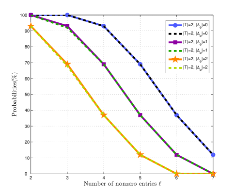
Figure 1: Comparison of theoretical and simulation results on recovery probability. Solid curves: probability curves of $\textbf{P}(\textbf{x}^{(1)}=\textbf{x}^{*};\|\textbf{x}^{*}\|_{0}=\ell,|\textbf{T}|=p,|\boldsymbol{\Delta}_{e}|=p_{1},\textbf{A})$ obtained by (4); dotted curves: probability curves obtained by a random sampling. The three pairs of solid and dotted curves from the top to the bottom correspond to $|\textbf{T}|=2$, $\left|{{\boldsymbol{\Delta}_{e}}}\right|=0$, 1, 2 respectively.

However, the computational burden to calculate (4) increases exponentially as the problem dimensions increase. As mentioned above, for each sign column vector and the corresponding index sets, we denote the quads $[\textbf{G}_{j}^{(\ell)},\textbf{N}_{s}^{(p_{2})},\textbf{H}_{i}^{(p_{1})},\textbf{t}_{\tau}]$, where $j=1,...,C_{n}^{\ell}$, $s=1,...,C_{\ell}^{p_{2}}$, $i=1,...,C_{n-\ell}^{p_{1}}$ and $\tau=1,...,2^{\ell-p_{2}}$. Suppose Z is a set composed by all the quads, there are $C_{n}^{\ell}C_{\ell}^{p_{2}}C_{n-\ell}^{p_{1}}2^{\ell-p_{2}}$ elements in Z. For each element of Z, if the sign column vector $\textbf{t}_{\tau}$ can be recovered by the modified-CS with a given matrix A and a known support $\textbf{T}=\textbf{N}_{s}^{(p_{2})}\cup\textbf{H}_{i}^{(p_{1})}$, we call the quad can be recovered. In (4), the estimation of recover probability need to check the total number of quads in Z. Hence, when $n$ increases, the computational burden will increase exponentially. To avoid this problem, we state the following Theorem.

Theorem 2

Suppose that $M$ quads are randomly taken from set Z, where $M$ is a large positive integer ($M\ll C_{n}^{\ell}C_{\ell}^{p_{2}}C_{n-\ell}^{p_{1}}2^{\ell-p_{2}}$), and $K$ of the $M$ quads can be recovered by solving modified-CS. Then

$${\bf{P}}({{\bf{x}}^{(1)}}={{\bf{x}}^{*}};{\left\|{{{\bf{x}}^{*}}}\right\|_{0}}=\ell,|{\bf{T}}|=p,\left|{{\boldsymbol{\Delta}_{e}}}\right|={p_{1}},{\bf{A}})\backsimeq\frac{K}{M}$$ (5)

The proof of this theorem is given in Appendix II.

Remark 3: In real-world applications, by sampling randomly $M$ sign vectors with $\ell$ nonzero entries, we can check the number of the vectors that can be exactly recovered by modified-CS with a random known support T whose size is $p$ but contains $p_{1}$ errors. Suppose $K$ sign vectors can be recovered, the recovery probability $\textbf{P}(\textbf{x}^{(1)}=\textbf{x}^{*};\|\textbf{x}^{*}\|_{0}=\ell,|\textbf{T}|=p,|\boldsymbol{\Delta}_{e}|=p_{1},\textbf{A})$ can be computed approximately through calculating the ratio of $K/M$.

From the proof of Theorem 2, the number of samples $M$, which controls the precision in the approximation of (5), is related to the two-point distribution of $\upsilon_{k}$ other than the size of Z. Thus, there is no need for $M$ increasing exponentially as $n$ increases. In the following example 2, this conclusion as well as the conclusion in Theorem (2) are demonstrated.

Example 2: In this example, according to the uniform distribution in [-0.5, 0.5], we randomly generate three matrices $\textbf{A}_{i}\in R^{m\times n}$ ($i=1,2,3$) with ($m$, $n$)=(7, 9), (52, 128) and (181, 1280) respectively. For matrices $\textbf{A}_{1}$, $\textbf{A}_{2}$ and $\textbf{A}_{3}$, we set ($\ell$, $p$, $p_{1}$)=(4, 2, 1), (20, 8, 3) and (60, 32, 4) respectively. As $n$ increases in the three cases, the number of sign vectors increases exponentially. For example, for $(m,n,\ell,p,p_{1})=(7,9,4,2,1)$ and $(52,128,20,8,3)$, the set Z contains approximately $2.02\times 10^{4}$ and $1.24\times 10^{37}$ elements respectively. Hence, for the three cases, we estimate the probabilities $\textbf{P}(\textbf{x}^{(1)}=\textbf{x}^{*};\|\textbf{x}^{*}\|_{0}=\ell,|\textbf{T}|=p,|\boldsymbol{\Delta}_{e}|=p_{1},\textbf{A})$ by (5). For each case, we sample $M$=100, 500, 1000, 5000, 10000 respectively. The resultant probability estimates depicted in Fig. 2 indicate that 1) the estimation precision of (5) is stable in our experiments with different number of samples. Therefore, we may just need very few samples to obtain the satisfied estimation precision in real-world applications; 2) as $n$ increases in three cases, the number of samples $M$ don’t need an exponential increase.

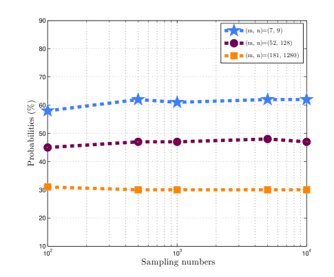
Figure 2: Probabilities curves obtained in example 2. The horizontal axis represents the sampling numbers. The vertical axis represents the probabilities $\textbf{P}(\textbf{x}^{(1)}=\textbf{x}^{*};\|\textbf{x}^{*}\|_{0}=\ell,|\textbf{T}|=p,|\boldsymbol{\Delta}_{e}|=p_{1},\textbf{A})$ obtained by (5).The three curves from the top to the bottom correspond to $(m,n,\ell,p,p_{1})=(7,9,4,2,1)$, $(52,128,20,8,3)$ and $(181,1280,60,32,4)$ respectively.

III Conclusion

In this letter we study the recoverability of the modified-CS in a stochastic framework. A sufficient and necessary condition on the recoverability is presented. Based on this condition, the recovery probability of the modified-CS can be estimated explicitly. It is worth mentioning that Theorem 1 can be easy to extend to the weighted-$\ell_{1}$ minimization approach that was proposed in [17] for nonuniform sparse model. Moreover, the recovery probability estimation provides alternative way to find (numerically) the optimal set of weights in the weighted-$\ell_{1}$ minimization approach, which has the largest recovery probability to recover the signals.

Appendix A Proof of Theorem 1

Proof:

Necessity: Suppose that $\textbf{x}^{(1)}=\textbf{x}^{*}$. Thus $\textbf{x}^{*}$ is the optimal solution and $\|\textbf{x}_{\textbf{T}^{c}}^{*}\|_{1}$ is the optimal value of the optimization problem in (2).

For a subset $\textbf{I}\in\textbf{F}$, when (3) is solvable, there is at least a feasible solution. For a feasible solution $\boldsymbol{\delta}$ of (3), it can be proved that $\textbf{x}^{*}+t\boldsymbol{\delta}$ is a solution of the constraint equation of (2), where $t$ is a constant. In the following, we suppose $t<0$ with sufficiently small absolute value. Then we have

$$\begin{split}{\left\|{\textbf{x}_{{\textbf{T}^{c}}}^{*}+t{\boldsymbol{\delta}_{{\textbf{T}^{c}}}}}\right\|_{1}}&=\sum\limits_{k\in\textbf{I}}{\left|{{x}_{k}^{*}+t{{\delta}_{k}}}\right|+\sum\limits_{k\in\boldsymbol{\Delta}\backslash\textbf{I}}{\left|{{x}_{k}^{*}+t{{\delta}_{k}}}\right|}}+\\ &\quad\sum\limits_{k\in{T^{c}\backslash\boldsymbol{\Delta}}}{\left|{t{{\delta}_{k}}}\right|}\\ &=\sum\limits_{k\in\textbf{I}}{\left|{{x}_{k}^{*}}\right|}-\left|t\right|\sum\limits_{k\in\textbf{I}}{\left|{{{\delta}_{k}}}\right|}+\sum\limits_{k\in\boldsymbol{\Delta}\backslash\textbf{I}}{\left|{{x}_{k}^{*}}\right|}+\\ &\quad\left|t\right|\sum\limits_{k\in\boldsymbol{\Delta}\backslash\textbf{I}}{\left|{{{\delta}_{k}}}\right|+\left|t\right|}\sum\limits_{k\in{T^{c}\backslash\boldsymbol{\Delta}}}{\left|{{{\delta}_{k}}}\right|}\\ &={\left\|{\textbf{x}_{{\textbf{T}^{c}}}^{*}}\right\|_{1}}+\left|t\right|(\sum\limits_{k\in({\textbf{T}^{c}}\backslash\textbf{I})}{\left|{{{\delta}_{k}}}\right|-\sum\limits_{k\in\textbf{I}}{\left|{{{\delta}_{k}}}\right|}})\end{split}$$ (6)

Since $\textbf{x}^{*}$ is the optimal solution of the optimization problem (2), it follows from (6) that

$${\left\|{\textbf{x}_{{\textbf{T}^{c}}}^{*}}\right\|_{1}}+\left|t\right|(\sum\limits_{k\in({\textbf{T}^{c}}\backslash\textbf{I})}{\left|{{{\delta}_{k}}}\right|-\sum\limits_{k\in\textbf{I}}{\left|{{{\delta}_{k}}}\right|}})>{\left\|{\textbf{x}_{{\textbf{T}^{c}}}^{*}}\right\|_{1}}$$ (7)

Thus,

$$\sum\limits_{k\in({\textbf{T}^{c}}\backslash\textbf{I})}{\left|{{{\delta}_{k}}}\right|-\sum\limits_{k\in\textbf{I}}{\left|{{{\delta}_{k}}}\right|}}>0$$ (8)

The necessity is proved.

Sufficiency: Suppose that $\textbf{x}^{{\dagger}}$ is a solution of the constraint equation in (2), which is different from $\textbf{x}^{*}$. Then $\textbf{x}^{{\dagger}}$ can be rewritten as

$$\textbf{x}^{{\dagger}}={\textbf{x}^{*}}+{t^{*}}\boldsymbol{\delta},$$ (9)

where $\boldsymbol{\delta}=\frac{{({\textbf{x}^{*}}-\textbf{x}^{{\dagger}})}}{{{{\left\|{{\textbf{x}^{*}}-\textbf{x}^{{\dagger}}}\right\|}_{1}}}}$, ${t^{*}}=-{\left\|{{\textbf{x}^{*}}-\textbf{x}^{{\dagger}}}\right\|_{1}}\not=0$.

Now we define an index set I,

$$\textbf{I}=\{k|k\in\boldsymbol{\Delta},\;sign({x}_{k}^{*})=sign({{\delta}_{k}})\}.$$ (10)

From (9), we have

$$\begin{split}{\left\|{\textbf{x}_{{\textbf{T}^{c}}}^{\dagger}}\right\|_{1}}&={\left\|{\textbf{x}_{{\textbf{T}^{c}}}^{*}+t^{*}{\boldsymbol{\delta}_{{\textbf{T}^{c}}}}}\right\|_{1}}\\ &=\sum\limits_{k\in\textbf{I}}{\left|{{x}_{k}^{*}+t^{*}{{\delta}_{k}}}\right|}+\sum\limits_{k\in\boldsymbol{\Delta}\backslash\textbf{I}}{\left|{{x}_{k}^{*}+t^{*}{{\delta}_{k}}}\right|}+\\ &\quad\sum\limits_{k\in{\textbf{T}^{c}\backslash\boldsymbol{\Delta}}}{\left|{t^{*}{{\delta}_{k}}}\right|}\\ &\geq\sum\limits_{k\in\textbf{I}}{\left|{{x}_{k}^{*}}\right|}-\left|t^{*}\right|\sum\limits_{k\in\textbf{I}}{\left|{{{\delta}_{k}}}\right|}+\sum\limits_{k\in\boldsymbol{\Delta}\backslash\textbf{I}}{\left|{{x}_{k}^{*}}\right|}+\\ &\quad\quad\quad\quad\left|t^{*}\right|\sum\limits_{k\in\boldsymbol{\Delta}\backslash\textbf{I}}{\left|{{{\delta}_{k}}}\right|+\left|t^{*}\right|}\sum\limits_{k\in{\textbf{T}^{c}\backslash\boldsymbol{\Delta}}}{\left|{{{\delta_{k}}}}\right|}\\ &={\left\|{\textbf{x}_{{\textbf{T}^{c}}}^{*}}\right\|_{1}}+\left|t^{*}\right|(\sum\limits_{k\in({\textbf{T}^{c}}\backslash\textbf{I})}{\left|{{{\delta}_{k}}}\right|-\sum\limits_{k\in\textbf{I}}{\left|{{{\delta}_{k}}}\right|}})\end{split}$$ (11)

It can be easily proved that for the defined index set I in (10), $\textbf{I}\in\textbf{F}$ and $\boldsymbol{\delta}$ is a feasible solution of (3). From the condition of the theorem, we have

$$\sum\limits_{k\in({\textbf{T}^{c}}\backslash\textbf{I})}{\left|{{{\delta}_{k}}}\right|-\sum\limits_{k\in\textbf{I}}{\left|{{{\delta}_{k}}}\right|}}>0.$$ (12)

Combining (11) and (12), we have

$${\left\|{\textbf{x}_{{\textbf{T}^{c}}}^{\dagger}}\right\|_{1}}>{\left\|{\textbf{x}_{{\textbf{T}^{c}}}^{*}}\right\|_{1}}.$$ (13)

Hence, $\textbf{x}^{*}$ is the optimal solution of (2). Thus, $\textbf{x}^{(1)}=\textbf{x}^{*}$. The sufficiency is proved. ∎

Appendix B Proof of Theorem 2

Proof:

Suppose Z can be split as $\textbf{Z}=\textbf{Z}_{e}\cup\textbf{Z}_{f}$, where $\textbf{Z}_{e}$ denotes the set composed by the $S_{w}$ quads that can be recovered, $\textbf{Z}_{f}=\textbf{Z}\setminus\textbf{Z}_{e}$. For a quad $\zeta$, we have

$$\textbf{P}(\zeta\in\textbf{Z}_{e})=\frac{S_{w}}{C_{n}^{\ell}C_{\ell}^{p_{2}}C_{n-\ell}^{p_{1}}2^{\ell-p_{2}}}$$ (14)

Now we define a sequence of random variables $\upsilon_{k}$ using the set of of quads $\textbf{Z}_{e}$

$$\upsilon_{k}=\left\{\begin{array}[]{ll}1,&\zeta_{k}\in\textbf{Z}_{e}\\ 0,&\zeta_{k}\in\textbf{Z}_{f}\end{array}\right.$$ (15)

where $k=1,2,...,\zeta_{k}$ is a quad randomly taken from Z.

From (14), it follows that $\textbf{P}(\upsilon_{k}=1)={S_{w}}/{C_{n}^{\ell}C_{\ell}^{p_{2}}C_{n-\ell}^{p_{1}}2^{\ell-p_{2}}}$, $\textbf{P}(\upsilon_{k}=0)=1-\textbf{P}(\upsilon_{k}=1)$. Therefore, $\upsilon_{k},k=1,2,...$ are independent and identically distributed random variables with the expected value $E(\upsilon_{k})={S_{w}}/{C_{n}^{\ell}C_{\ell}^{p_{2}}C_{n-\ell}^{p_{1}}2^{\ell-p_{2}}}$.

According to the law of large numbers (Bernoulli) in probability theory, the sample average $(1/M)\sum\nolimits_{i=1}^{M}{{V_{i}}}=K/M$ converges towards the expected value $E(\upsilon_{k})$, where ${V_{i}}$ is a sample of the random variable $\upsilon_{k}$. It follows that when $M$ is sufficiently large

$$E(\upsilon_{k})={S_{w}}/{C_{n}^{\ell}C_{\ell}^{p_{2}}C_{n-\ell}^{p_{1}}2^{\ell-p_{2}}}\backsimeq\frac{K}{M}$$ (16)

The theorem is proven. ∎

References

• [1] D. L. Donoho, “Compressed sensing,” IEEE Trans. Inf. Theory, vol. 52, no. 4, pp. 1289–1306, 2006.
• [2] E. J. Candès, J. Romberg, and T. Tao, “Robust uncertainty principles: exact signal reconstruction from highly incomplete frequency information,” IEEE Trans. Inf. Theory, vol. 52, no. 2, pp. 489–509, 2006.
• [3] E. J. Candès and T. Tao, “Near-optimal signal recovery from random projections: universal encoding strategies?” IEEE Trans. Inf. Theory, vol. 52, no. 12, pp. 5406–5425, 2006.
• [4] S. S. Chen, D. L. Donoho, and M. A. Saunders, “Atomic decomposition by basis pursuit,” SIAM REV., vol. 43, no. 1, pp. 129–159, 2001.
• [5] E. Candes and T. Tao, “Decoding by linear programming,” IEEE Trans. Inf. Theory, vol. 51, no. 12, pp. 4203–4215, 2005.
• [6] N. Vaswani and W. Lu, “Modified-CS : modifying compressive sensing for problems with partially known support,” IEEE Trans. Signal Process., vol. 58, no. 9, pp. 4595–4607, 2010.
• [7] ——, “Modified-CS: modifying compressive sensing for problems with partially known support,” in Proc. IEEE Int. Symp. Inf. Theory (ISIT), 2009, pp. 488–492.
• [8] W. Lu and N. Vaswani, “Modified compressive sensing for real-time dynamic mr imaging,” in Proc. IEEE Int. Conf. Image Proc. (ICIP), 2009, pp. 3009–3012.
• [9] C. Qiu, W. Lu, and N. Vaswani, “Real-time dynamic mri reconstruction using kalman filtered cs,” in Proc. Int. Conf. Acoustics, Speech, Signal Processing(ICASSP), 2009, pp. 393–396.
• [10] C. Miosso, R. von Borries, M. Argàez, L. Velazquez, C. Quintero, and C. Potes, “Compressive sensing reconstruction with prior information by iteratively reweighted least-squares,” IEEE Trans. Signal Process., vol. 57, no. 6, pp. 2424–2431, 2009.
• [11] R. von Borries, C. Miosso, and C. Potes, “Compressed sensing using prior information,” in Computational Advances in Multi-Sensor Adaptive Processing, 2007. CAMPSAP 2007. 2nd IEEE International Workshop on, 2007, pp. 121–124.
• [12] Y. Wang and W. Yin, “sparse signal reconstruction via iterative support detection,” SIAM J Imag. Sci., vol. 3, no. 3, pp. 462–491, 2010.
• [13] W. Guo and W. Yin, “Edgecs: edge guided compressive sensing reconstruction,” Department of Computational and Applied Mathmatics, Rice University, Houston, TX, Tech. Rep. TR10-02, Jan. 2010.
• [14] M. Friedlander, H. Mansour, R. Saab, and O. Yilmaz, “Recovering compressively sampled signals using partial support information,” to appear in the IEEE Trans. Inf. Theory, 2010.
• [15] L. Jacques, “A short note on compressed sensing with partially known signal support,” Signal Processing, vol. 90, no. 12, pp. 3308–3312, 2010.
• [16] Y. Li, S. Amari, A. Cichocki, and C. Guan, “Probability estimation for recoverability analysis of blind source separation based on sparse representation,” IEEE Trans. Inf. Theory, vol. 52, no. 7, pp. 3139–3152, 2006.
• [17] M. Khajehnejad, W. Xu, S. Avestimehr, and B. Hassibi, “Analyzing weighted $\ell_{1}$ minimization for sparse recovery with nonuniform sparse models,” IEEE Trans. Signal Process., vol. 59, no. 5, pp. 1985–2001, 2011.