A Symmetry-based Decomposition Approach to Eigenvalue Problems: Formulation, Discretization, and Implementation

Abstract. In this paper, we propose a decomposition approach for eigenvalue problems with spatial symmetries, including the formulation, discretization as well as implementation. This approach can handle eigenvalue problems with either Abelian or non-Abelian symmetries, and is friendly for grid-based discretizations such as finite difference, finite element or finite volume methods. With the formulation, we divide the original eigenvalue problem into a set of subproblems and require only a smaller number of eigenpairs for each subproblem. We implement the decomposition approach with finite elements and parallelize our code in two levels. We show that the decomposition approach can improve the efficiency and scalability of iterative diagonalization. In particular, we apply the approach to solving Kohn–Sham equations of symmetric molecules consisting of hundreds of atoms.

Keywords. Eigenvalue, Grid-based discretization, Symmetry, Group theory, Two-level parallelism.

1 Introduction

Efficient numerical methods for differential eigenvalue problems become significant in scientific and engineering computations. For instance, many properties of molecular systems or solid-state materials are determined by solving Schrödinger-type eigenvalue problems, such as Hartree–Fock or Kohn–Sham equations [11, 38, 53]; the vibration analysis of complex structures is achieved by solving the eigenvalue problems derived from the equation of motion [7, 16, 31]. We understand that a lot of eigenpairs have to be computed when the size of the molecular system is large in electronic structure study, or the frequency range of interest is increased in structural analysis. To obtain accurate approximations, we see that a large number of degrees of freedom should be employed in discretizations.

Since the computational cost grows in proportion to $N_{e}^{2}N$, where $N_{e}$ is the number of required eigenpairs and $N$ the number of degrees of freedom, we should decompose such large-scale eigenvalue problems over domain or over required eigenpairs. However, it is not easy to decompose an eigenvalue problem because the problem has an intrinsic nonlinearity and is set as a global optimization problem with orthonormal constraints. We observe that the existing efficient domain decomposition methods for boundary value problems usually do not work well for eigenvalue problems.

For an eigenvalue problem with symmetries, we are happy to see that the symmetries may provide a way to do decomposition. Mathematically, each symmetry corresponds to an operator, such as a reflection, a rotation or an inversion, that leaves the object or problem invariant. Group theory provides a systematic way to exploit symmetries [8, 14, 15, 33, 47, 52]. Using group representation theory, we may decompose the eigenspace into some orthogonal subspaces. More precisely, the decomposed subspaces have distinct symmetries and are orthogonal to each other. However, there are real difficulties in the implementation of using symmetries [5, 10].

We see from quantum physics and quantum chemistry that people use the so-called symmetry-adapted bases to approximate eigenfunctions in such orthogonal subspaces. The symmetry-adapted bases are constructed from specific basis functions like atomic orbitals, internal coordinates of a molecule, or orthogonalized plane waves [8, 14, 15]. A case-by-case illustration of the way to construct these bases from atomic orbitals has been given in [15], from which we can see that the construction of symmetry-adapted bases is not an easy task.

We observe that grid-based discretizations, such as finite difference, finite element and finite volume methods, are widely used in scientific and engineering computations [3, 4, 12, 18, 27]. For instance, the finite element method is often used to discretize eigenvalue problems in structural analysis [7, 31, 55]. In the last two decades, grid-based discretization approaches have been successfully applied to modern electronic structure calculations, see [6, 17, 43, 48] and reference cited therein. In particular, grid-based discretizations have good locality and have been proven to be well accommodated to peta-scale computing by treating extremely large-scale eigenvalue problems arising from the electron structure calculations [28, 32]. Note that grid-based discretizations usually come with a large number of degrees of freedom. And finite difference methods do not have basis functions in the classical sense. These facts increase the numerical difficulty to construct symmetry-adapted bases.

In this paper, we propose a new decomposition approach to differential eigenvalue problems with symmetries, which is friendly for grid-based discretizations and does not need the explicit construction of symmetry-adapted bases. We decompose an eigenvalue problem with Abelian or non-Abelian symmetries into a set of eigenvalue subproblems characterized by distinct conditions derived from group representation theory. We use the characteristic conditions directly in grid-based discretizations to form matrix eigenvalue problems. Beside the decomposition approach, we provide a construction procedure for the symmetry-adapted bases. Then we illustrate the equivalence between our approach and the approach that constructs symmetry-adapted bases, by deducing the exact relation between the two discretized problems.

We implement the decomposition approach based on finite element discretizations. Subproblems corresponding to different irreducible representations can be solved independently. Accordingly, we parallelize our code in two levels, including a fundamental level of spatial parallelization and another level of subproblem distribution. We apply the approach to solving the Kohn–Sham equation of some cluster systems with symmetries. Our computations show that the decomposition approach would be appreciable for large-scale eigenvalue problems. The implementation techniques can be adapted to finite difference and finite volume methods, too.

The computational overhead and memory requirement can be reduced by our decomposition approach. Required eigenpairs for the original problem are distributed among subproblems; namely, only a smaller number of eigenpairs are needed for each subproblem. And subproblems can be solved in a small subdomain. Here we give an example to illustrate the effectiveness of the decomposition approach. Consider the eigenvalue problem for the Laplacian in domain $(-1,1)^{3}$ with zero boundary condition, and solve the first 1000 smallest eigenvalues and associated eigenfunctions. We decompose the eigenvalue problem into 8 decoupled eigenvalue subproblems by applying Abelian group $D_{2h}$ which has 8 symmetry operations. The number of computed eigenpairs for each subproblem is 155, and the number of degrees of freedom for solving each subproblem, 205,379, is one eighth of that for the original problem, 1,643,032. We obtain a speedup of 28.8 by solving 8 subproblems instead of the original problem.

We should mention that group theory has been introduced to partial differential equations arising from structural analysis in [9, 10], which mainly focused on boundary value problems and did not provide any numerical result. We understand that the design and implementation of decomposition methods for eigenvalue problems are different from boundary value problems. We also see that Abelian symmetries have been utilized to simplify the solving of Kohn–Sham equations in a finite difference code [35]. However, the implementation in [35] is only applicable to Abelian groups, in which any two symmetry operations are commutative. Even in quantum chemistry, most software packages only utilize Abelian groups [53]. In some plane-wave softwares of electronic structure calculations, symmetries are used to simplify the solving of Kohn–Sham equations by reducing the number of $k$-points to the irreducible Brillouin zone (IBZ). For a given $k$-point, they do not classify the eigenstates and thus still solve the original eigenvalue problem.

The rest of this paper is organized as follows. In Section 2, we show the symmetry-based decomposition of eigenvalue problems, and propose a subproblem formulation proper for grid-based discretizations. Then in Section 3, we give matrix eigenvalue problems derived from the subproblem formulation and provide a construction procedure for the symmetry-adapted bases, from which we deduce the relation of our discretized problems to those formed by symmetry-adapted bases. We quantize the decrease in computational cost when using the decomposition approach in Section 4. And in Section 5 we present some critical implementation issues. In Section 6, we give numerical examples to validate our implementation for Abelian and non-Abelian symmetry groups and show the reduction in computational and communicational overhead; then we apply the decomposition approach to solving the Kohn–Sham equation of three symmetric molecular systems with hundreds of atoms. Finally, we give some concluding remarks.

2 Decomposition formulation

In this section, we recall several basic but useful results of group theory and propose a symmetry-based decomposition formulation. The formulation, summarized as Theorem 2.1 and Corollary 2.2, can handle eigenvalue problems with Abelian or non-Abelian symmetries. Some notation and concepts will be given in Appendix A.

2.1 Representation, basis function, and projection operator

We start from orthogonal coordinate transformations in $\mathbb{R}^{d}~{}(d=1,2,3)$ such as a rotation, a reflection or an inversion, that form a finite group $G$ of order $g$. Let $\Omega\subset\mathbb{R}^{d}$ be a bounded domain and $V\subset L^{2}(\Omega)$ a Hilbert space of functions on $\Omega$ equipped with the $L^{2}$ scalar product $(\cdot,\cdot)$. Each $R\in G$ corresponds to an operator $P_{R}$ on $f\in V$ as

$$P_{R}f(Rx)=f(x)\quad\forall x\in\Omega.$$

It is proved that $\{P_{R}:R\in G\}$ form a group isomorphic to $G$.

A matrix representation of group $G$ means a group of matrices which is homomorphic to $G$. Any matrix representation with nonvanishing determinants is equivalent to a representation by unitary matrices (referred to as unitary representation). In the following we focus on unitary representations of group $G$.

The great orthogonality theorem (cf. [14, 33, 47, 52]) tells that, all the inequivalent, irreducible, unitary representations $\{\Gamma^{(\nu)}\}$ of group $G$ satisfy

$$\sum_{R\in G}{\Gamma^{(\nu)}(R)}^{*}_{ml}\Gamma^{(\nu^{\prime})}(R)_{m^{\prime}l^{\prime}}=\delta_{\nu\nu^{\prime}}\delta_{mm^{\prime}}\delta_{ll^{\prime}}\frac{g}{d_{\nu}}$$ (2.1)

for any $l,m\in\{1,2,\ldots,d_{\nu}\}$ and $l^{\prime},m^{\prime}\in\{1,2,\ldots,d_{\nu^{\prime}}\}$, where $d_{\nu}$ denotes the dimensionality of the $\nu$-th representation $\Gamma^{(\nu)}$ and ${\Gamma^{(\nu)}(R)}^{*}_{ml}$ is the complex conjugate of $\Gamma^{(\nu)}(R)_{ml}$. The number of all the inequivalent, irreducible, unitary representations is equal to the number of classes in $G$. We denote this number as $n_{c}$.

Definition 2.1.

Given $\nu\in\{1,2,\ldots,n_{c}\}$, non-zero functions $\{\phi^{(\nu)}_{l}:l=1,2,\ldots,d_{\nu}\}\subset V$ are said to form a basis for $\Gamma^{(\nu)}$ if for any $l\in\{1,2,\ldots,{d_{\nu}}\}$

$$P_{R}\phi^{(\nu)}_{l}=\sum_{m=1}^{d_{\nu}}\phi^{(\nu)}_{m}\Gamma^{(\nu)}(R)_{ml}\quad\forall R\in G.$$ (2.2)

Function $\phi^{(\nu)}_{l}$ is called to belong to the $l$-th column of $\Gamma^{(\nu)}$ (or adapt to the $\nu$-$l$ symmetry), and $\{\phi^{(\nu)}_{m}:m=1,2,\ldots,d_{\nu},m\neq l\}$ are its partners.

There holds an orthogonality property for the basis functions (cf. [47, 52]): if $\{\phi^{(\nu)}_{l}:l=1,2,\ldots,d_{\nu}\}$ and $\{\psi^{(\nu^{\prime})}_{l^{\prime}}:l^{\prime}=1,2,\ldots,d_{\nu^{\prime}}\}$ are basis functions for irreducible representations $\Gamma^{(\nu)}$ and $\Gamma^{(\nu^{\prime})}$, respectively, then

$$(\phi_{l}^{(\nu)},\psi_{l^{\prime}}^{(\nu^{\prime})})=\delta_{\nu\nu^{\prime}}\delta_{ll^{\prime}}d_{\nu}^{-1}\sum_{m=1}^{d_{\nu}}(\phi_{m}^{(\nu)},\psi_{m}^{(\nu)})$$ (2.3)

holds for any $l\in\{1,2,\ldots,d_{\nu}\}$ and $l^{\prime}\in\{1,2,\ldots,d_{\nu^{\prime}}\}$. This equation implies that, two functions are orthogonal if they belong to different irreducible representations or to different columns of the same unitary representation. And the scalar product of two functions belonging to the same column of a given unitary representation (or adapting to the same symmetry) is independent of the column label.

Multiplying equation (2.2) by ${\Gamma^{(\nu^{\prime})}(R)}^{*}_{m^{\prime}l^{\prime}}$ and summing over $R$, the great orthogonality theorem (2.1) implies that

$$\sum_{R\in G}{\Gamma^{(\nu^{\prime})}(R)}^{*}_{m^{\prime}l^{\prime}}P_{R}\phi^{(\nu)}_{l}=\delta_{\nu\nu^{\prime}}\delta_{ll^{\prime}}\frac{g}{d_{\nu}}\phi^{(\nu)}_{m^{\prime}}\quad\forall~{}l^{\prime},m^{\prime}\in\{1,2,\ldots,d_{\nu^{\prime}}\},~{}l\in\{1,2,\ldots,{d_{\nu}}\}.$$

Define for any $\nu\in\{1,2,\ldots,n_{c}\}$ and $l,m\in\{1,2,\ldots,d_{\nu}\}$ operator $\mathscr{P}^{(\nu)}_{ml}$ as

$$\mathscr{P}^{(\nu)}_{ml}=\frac{d_{\nu}}{g}\sum_{R\in G}{\Gamma^{(\nu)}(R)}^{*}_{ml}P_{R},$$ (2.4)

we get

$$\mathscr{P}^{(\nu)}_{ml}\phi^{(\nu^{\prime})}_{l^{\prime}}=\delta_{\nu\nu^{\prime}}\delta_{ll^{\prime}}\phi^{(\nu)}_{m}$$ (2.5)

for any $\nu,\nu^{\prime}\in\{1,2,\ldots,n_{c}\}$, $l,m\in\{1,2,\ldots,d_{\nu}\}$, and $l^{\prime}\in\{1,2,\ldots,{d_{\nu^{\prime}}}\}$.

Proposition 2.1.

Given $\nu\in\{1,2,\ldots,n_{c}\}$ and $k\in\{1,2,\ldots,d_{\nu}\}$. If $v\in V$ satisfies $\mathscr{P}^{(\nu)}_{kk}v\neq 0$, then $\{\mathscr{P}^{(\nu)}_{lk}v:l=1,2,\ldots,d_{\nu}\}$ form a basis for $\Gamma^{(\nu)}$, i.e., $\{\mathscr{P}^{(\nu)}_{lk}v:l=1,2,\ldots,d_{\nu}\}$ are non-zero functions, and for any $l\in\{1,2,\ldots,d_{\nu}\}$

$$P_{R}\left(\mathscr{P}^{(\nu)}_{lk}v\right)=\sum_{m=1}^{d_{\nu}}\left(\mathscr{P}^{(\nu)}_{mk}v\right)\Gamma^{(\nu)}(R)_{ml}\quad\forall R\in G.$$

Proof.

For any $l\in\{1,2,\ldots,d_{\nu}\}$, we obtain from (2.4) that

$$P_{R}\left(\mathscr{P}^{(\nu)}_{lk}v\right)=\frac{d_{\nu}}{g}\sum_{S\in G}{\Gamma^{(\nu)}(S)}^{*}_{lk}P_{RS}~{}v=\frac{d_{\nu}}{g}\sum_{S^{\prime}\in G}{\Gamma^{(\nu)}(R^{-1}S^{\prime})}^{*}_{lk}P_{S^{\prime}}v\quad\forall R\in G,$$

where $P_{R}P_{S}=P_{RS}$ because $\{P_{R}:R\in G\}$ form a group isomorphic to $G$.

Since $\Gamma^{(\nu)}$ is a unitary representation of $G$, we have

$$P_{R}\left(\mathscr{P}^{(\nu)}_{lk}v\right)=\frac{d_{\nu}}{g}\sum_{S^{\prime}\in G}\left(\sum_{m=1}^{d_{\nu}}\Gamma^{(\nu)}(R)_{ml}{\Gamma^{(\nu)}(S^{\prime})}^{*}_{mk}\right)P_{S^{\prime}}v,$$

or

$$P_{R}\left(\mathscr{P}^{(\nu)}_{lk}v\right)=\sum_{m=1}^{d_{\nu}}\left(\mathscr{P}^{(\nu)}_{mk}v\right)\Gamma^{(\nu)}(R)_{ml}\quad\forall R\in G.$$

Recall the way to achieve (2.5), we see from the above equation and the great orthogonality theorem that

$$\mathscr{P}^{(\nu)}_{kk}v=\mathscr{P}^{(\nu)}_{kl}\left(\mathscr{P}^{(\nu)}_{lk}v\right)\quad\forall~{}l\in\{1,2,\ldots,d_{\nu}\}.$$

So $\mathscr{P}^{(\nu)}_{kk}v\neq 0$ indicates $\mathscr{P}^{(\nu)}_{lk}v\neq 0$ for all $l\in\{1,2,\ldots,d_{\nu}\}$. This completes the proof.   ∎

If we set $\nu^{\prime}=\nu$, $l^{\prime}=l$ and $m=l$ in (2.5), then we have for any $\nu\in\{1,2,\ldots,n_{c}\}$

$$\mathscr{P}^{(\nu)}_{ll}\phi^{(\nu)}_{l}=\phi^{(\nu)}_{l}\quad\forall~{}l\in\{1,2,\ldots,d_{\nu}\}.$$ (2.6)

Proposition 2.1 implies that (2.6) serves to characterize the labels of any basis function:

Corollary 2.1.

Given $\nu\in\{1,2,\ldots,n_{c}\}$ and $l\in\{1,2,\ldots,d_{\nu}\}$. Non-zero function $v\in V$ belongs to the $l$-th column of $\Gamma^{(\nu)}$ (or adapts to the $\nu$-$l$ symmetry) if and only if

$$\mathscr{P}^{(\nu)}_{ll}v=v.$$

We will use the following properties of operator $\mathscr{P}^{(\nu)}_{ml}$, whose proof is given in Appendix B.

Proposition 2.2.

Let $\nu,\nu^{\prime}\in\{1,2,\ldots,n_{c}\}$, $l,m\in\{1,2,\ldots,d_{\nu}\}$, and $l^{\prime},m^{\prime}\in\{1,2,\ldots,d_{\nu^{\prime}}\}$.

(a) The adjoint of operator $\mathscr{P}^{(\nu)}_{ml}$ satisfies

$${\mathscr{P}^{(\nu)}_{ml}}^{*}=\mathscr{P}^{(\nu)}_{lm}.$$

(b) The multiplication of two operators $\mathscr{P}^{(\nu)}_{ml}$ and $\mathscr{P}^{(\nu^{\prime})}_{m^{\prime}l^{\prime}}$ satisfies

$$\mathscr{P}^{(\nu)}_{ml}\mathscr{P}^{(\nu^{\prime})}_{m^{\prime}l^{\prime}}=\delta_{\nu\nu^{\prime}}\delta_{lm^{\prime}}\mathscr{P}^{(\nu)}_{ml^{\prime}}.$$

2.2 Subproblems

We see from Corollary 2.1 and the linearity of operator $\mathscr{P}^{(\nu)}_{ll}$ that, all functions in $V$ belonging to the $l$-th column of $\Gamma^{(\nu)}$ (or adapting to the $\nu$-$l$ symmetry) form a subspace of $V$. We denote this subspace by $V_{l}^{(\nu)}$.

There holds a decomposition theorem for any function in $V$ (cf. [47, 52]): any $f\in V$ can be decomposed into a sum of the form

$$f=\sum_{\nu=1}^{n_{c}}\sum_{l=1}^{d_{\nu}}f_{l}^{(\nu)},$$ (2.7)

where $f_{l}^{(\nu)}\in V_{l}^{(\nu)}$. We see from (2.5) and (2.7) that $\mathscr{P}^{(\nu)}_{ll}:V\rightarrow V_{l}^{(\nu)}$ is a projection operator. Equation (2.7) implies

$$V=\sum_{\nu=1}^{n_{c}}\sum_{l=1}^{d_{\nu}}V_{l}^{(\nu)},$$

which indeed is a direct sum

$$V=\bigoplus_{\nu=1}^{n_{c}}\bigoplus_{l=1}^{d_{\nu}}V_{l}^{(\nu)}$$ (2.8)

due to (2.3).

Now we turn to study the symmetry-based decomposition for eigenvalue problems. Consider eigenvalue problems of the form

$$Lu=\lambda u\quad\mbox{in}~{}\Omega$$ (2.9)

subject to some boundary condition, where $L$ is an Hermitian operator. Group $G$ is said to be a symmetry group associated with eigenvalue problem (2.9) if

$$R\Omega=\Omega,~{}P_{R}L=LP_{R}\quad\forall R\in G,$$

and the subjected boundary condition is also invariant under $\{P_{R}\}$. Then any $R\in G$ is called a symmetry operation for problem (2.9). For simplicity, we take zero boundary condition as an example and discuss the decomposition of eigenvalue problem

$$\left\{\begin{array}[]{rcll}Lu&=&\lambda u&\quad\mbox{in}~{}\Omega,\\ u&=&0&\quad\mbox{on}~{}\partial\Omega.\end{array}\right.$$ (2.10)

Since $P_{R}$ and $L$ are commutative for any $R$ in $G$, we have:

Proposition 2.3.

If $v\in V_{l}^{(\nu)}$, then $Lv\in V_{l}^{(\nu)}$, where $\nu\in\{1,2,\ldots,n_{c}\}$ and $l\in\{1,2,\ldots,d_{\nu}\}$. In other words, $V_{l}^{(\nu)}$ is an invariant subspace of operator $L$.

The direct sum decomposition of space $V$ and Proposition 2.3 indicate a decomposition of the eigenvalue problem.

Theorem 2.1.

Suppose finite group $G=\{R\}$ is a symmetry group associated with eigenvalue problem (2.10). Denote all the inequivalent, irreducible, unitary representations of $G$ as $\{\Gamma^{(\nu)}:\nu=1,2,\ldots,n_{c}\}$. Then the eigenvalue problem can be decomposed into $\sum_{\nu=1}^{n_{c}}d_{\nu}$ subproblems. For any $\nu\in\{1,2,\ldots,n_{c}\}$, the corresponding $d_{\nu}$ subproblems are

$$\left\{\begin{array}[]{rcll}Lu_{l}^{(\nu)}&=&\lambda^{(\nu)}u_{l}^{(\nu)}&\quad\mbox{in}~{}\Omega,\\ u_{l}^{(\nu)}&=&0&\quad\mbox{on}~{}\partial\Omega,\qquad l=1,2,\ldots,d_{\nu},\\ u_{l}^{(\nu)}&=&\mathscr{P}^{(\nu)}_{lk}u_{k}^{(\nu)}&\quad\mbox{in}~{}\Omega,\end{array}\right.$$ (2.11)

where $k$ is any chosen number in $\{1,2,\ldots,d_{\nu}\}$.

Proof.

We see from (2.8) and Proposition 2.3 that, other than solving the eigenvalue problem in $V$, we can solve the problem in each subspace $V_{l}^{(\nu)}$ independently. More precisely, we can decompose the original eigenvalue problem (2.10) into $\sum_{\nu=1}^{n_{c}}d_{\nu}$ subproblems; for any $\nu\in\{1,2,\ldots,n_{c}\}$, the $d_{\nu}$ subproblems are as follows

$$\left\{\begin{array}[]{rcll}Lu_{l}^{(\nu)}&=&\lambda_{l}^{(\nu)}u_{l}^{(\nu)}&\quad\mbox{in}~{}\Omega,\\ u_{l}^{(\nu)}&=&0&\quad\mbox{on}~{}\partial\Omega,\qquad l=1,2,\ldots,d_{\nu},\\ \mathscr{P}^{(\nu)}_{ll}u_{l}^{(\nu)}&=&u_{l}^{(\nu)}&\quad\mbox{in}~{}\Omega,\end{array}\right.$$ (2.12)

where the third equation characterizes $u_{l}^{(\nu)}\in V_{l}^{(\nu)}$, as indicated in Corollary 2.1.

Given any $\nu\in\{1,2,\ldots,n_{c}\}$, we consider the $d_{\nu}$ subproblems (2.12). We shall prove that, for any $k,l\in\{1,2,\ldots,d_{\nu}\}$, if $v$ and $w$ are two orthogonal eigenfunctions corresponding to some eigenvalue of the $k$-th subproblem, then $\mathscr{P}^{(\nu)}_{lk}v$ and $\mathscr{P}^{(\nu)}_{lk}w$ are eigenfunctions of the $l$-th subproblem with the same eigenvalue, and are also orthogonal.

Combining (2.5) and the fact that $P_{R}$ and $L$ are commutative for each $R$, we obtain that $\mathscr{P}^{(\nu)}_{lk}v$ is an eigenfunction of the $l$-th subproblem which corresponds to the same eigenvalue as the one for $v$. It remains to prove the orthogonality of $\mathscr{P}^{(\nu)}_{lk}v$ and $\mathscr{P}^{(\nu)}_{lk}w$. Proposition 2.2 indicates that the scalar product of any two functions in $V_{k}^{(\nu)}$ is invariant after operating on them with $\mathscr{P}^{(\nu)}_{lk}$. Indeed, we have for any $v,w\in V_{k}^{(\nu)}$ that

$$(\mathscr{P}^{(\nu)}_{lk}v,\mathscr{P}^{(\nu)}_{lk}w)=(\mathscr{P}^{(\nu)*}_{lk}\mathscr{P}^{(\nu)}_{lk}v,w)=(\mathscr{P}^{(\nu)}_{kl}\mathscr{P}^{(\nu)}_{lk}v,w)=(\mathscr{P}^{(\nu)}_{kk}v,w),$$

which together with Corollary 2.1 leads to

$$(\mathscr{P}^{(\nu)}_{lk}v,\mathscr{P}^{(\nu)}_{lk}w)=(v,w).$$

Thus $\mathscr{P}^{(\nu)}_{lk}v$ and $\mathscr{P}^{(\nu)}_{lk}w$ are orthogonal when $v$ and $w$ are.

Since $L$ is Hermitian, we see that for the $d_{\nu}$ subproblems (2.12), eigenvalues of the $l$-th subproblem are the same as those of the $k$-th one, and eigenfunctions of the $l$-th subproblem can be chosen as $\{\mathscr{P}^{(\nu)}_{lk}v\}$, where $\{v\}$ are eigenfunctions of the $k$-th subproblem and $k$ is any chosen number in $\{1,2,\ldots,d_{\nu}\}$.

Therefore, the original eigenvalue problem (2.10) is decomposed into $\sum_{\nu=1}^{n_{c}}d_{\nu}$ subproblems, and for any $\nu\in\{1,2,\ldots,n_{c}\}$ the corresponding $d_{\nu}$ subproblems can be given as (2.11). This completes the proof.   ∎

The third equation of the $d_{\nu}$ subproblems in (2.11) are

$$u_{k}^{(\nu)}=\mathscr{P}^{(\nu)}_{kk}u_{k}^{(\nu)},$$

$$u_{l}^{(\nu)}=\mathscr{P}^{(\nu)}_{lk}u_{k}^{(\nu)}\quad\forall~{}l=1,2,\ldots,d_{\nu},~{}l\neq k.$$

We see from Proposition 2.1 that $\{u_{l}^{(\nu)}:l=1,2,\ldots,d_{\nu}\}$ form a basis for $\Gamma^{(\nu)}$. Namely, for any $l\in\{1,2,\ldots,d_{\nu}\}$

$$P_{R}u_{l}^{(\nu)}=\sum_{m=1}^{d_{\nu}}u_{m}^{(\nu)}~{}\Gamma^{(\nu)}(R)_{ml}\quad\forall R\in G,$$

i.e.,

$$u_{l}^{(\nu)}(Rx)=\sum_{m=1}^{d_{\nu}}{\Gamma^{(\nu)}(R)}^{*}_{lm}u_{m}^{(\nu)}(x)\quad\forall R\in G.$$

Corollary 2.2.

Under the same condition as in Theorem 2.1, eigenvalue problem (2.10) can be decomposed into $\sum_{\nu=1}^{n_{c}}d_{\nu}$ subproblems. For any $\nu\in\{1,2,\ldots,n_{c}\}$, the corresponding $d_{\nu}$ subproblems can be given as follows

$$\qquad\left\{\begin{array}[]{rcll}Lu_{l}^{(\nu)}&=&\lambda^{(\nu)}u_{l}^{(\nu)}&~{}~{}\mbox{in}~{}\Omega,\\ u_{l}^{(\nu)}&=&0&~{}~{}\mbox{on}~{}\partial\Omega,\qquad\qquad l=1,2,\ldots,d_{\nu}.\\ u_{l}^{(\nu)}(Rx)&=&{\displaystyle\sum_{m=1}^{d_{\nu}}}{\Gamma^{(\nu)}(R)}^{*}_{lm}u_{m}^{(\nu)}(x)&~{}~{}\mbox{in}~{}\Omega,~{}\forall R\in G,\end{array}\right.$$ (2.13)

The third equations in (2.11) and (2.13) describe symmetry properties of eigenfunctions over domain $\Omega$. The original eigenvalue problem can be decomposed into subproblems just because eigenfunctions of subproblems satisfy distinct equations. In the following text, we call these equations as symmetry characteristics.

Denote by $\Omega_{0}$ the smallest subdomain which produces $\Omega$ by applying all symmetry operations $\{R\in G\}$, namely, ${\bar{\Omega}}=\cup_{R\in G}\overline{R\Omega_{0}}$, and ${R_{1}\Omega_{0}}\cap{R_{2}\Omega_{0}}=\varnothing$ for any $R_{1},R_{2}\in G$ satisfying $R_{1}\neq R_{2}$. We call $\Omega_{0}$ the irreducible subdomain and the associated volume is $g$ times smaller than that of $\Omega$. The symmetry characteristic equation in (2.13) tells that for any $l\in\{1,2,\ldots,d_{\nu}\}$, $u_{l}^{(\nu)}$ over $\Omega$ is determined by the values of functions $\{u_{1}^{(\nu)},\ldots,u_{d_{\nu}}^{(\nu)}\}$ over $\Omega_{0}$. So each subproblem can be solved over $\Omega_{0}$.

Remark 2.1.

A decomposition formulation has been shown in [10] for boundary value problems with spatial symmetries. Each decomposed problem is characterized by a “boundary condition” on $\Sigma_{g}$ , which is in fact a restriction of the symmetry characteristic on boundary $\Sigma_{g}$. Indeed, symmetry characteristics over $\Omega$ should not be replaced by the restriction on the internal boundary. In some cases, it is true that boundary conditions such as Dirichlet or Neumann type can be deduced, while in the deduction of Neumann boundary conditions one has to use the symmetry characteristic near the internal boundary, not only on the boundary. In some other cases, symmetry characteristics may not produce proper boundary conditions.

2.3 An example

We take the Laplacian in square $(-1,1)^{2}$ as an example to illustrate the subproblem formulation in Corollary 2.2. Namely, we consider the decomposition of the following eigenvalue problem

$$\left\{\begin{array}[]{rcll}-\Delta u&=&\lambda u&\quad\mbox{in}~{}\Omega=(-1,1)^{2},\\ u&=&0&\quad\mbox{on}~{}\partial\Omega.\end{array}\right.$$ (2.14)

Note that $G=\{E,\sigma_{x},\sigma_{y},I\}$ is a symmetry group associated with (2.14), where $E$ represents the identity operation, $\sigma_{x}$ a reflection about $x$-axis, $\sigma_{y}$ a reflection about $y$-axis, and $I$ the inversion operation. We see that $G$ is an Abelian group of order 4, and has 4 one-dimensional irreducible representations as shown in Table 1.

Table 1: Representation matrices of example group $G$.

$G$	$R_{1}=E$	$R_{2}=\sigma_{x}$	$R_{3}=\sigma_{y}$	$R_{4}=I$
$\Gamma^{(1)}$	1	1	1	1
$\Gamma^{(2)}$	1	1	-1	-1
$\Gamma^{(3)}$	1	-1	-1	1
$\Gamma^{(4)}$	1	-1	1	-1

According to Theorem 2.1 and Corollary 2.2, eigenvalue problem (2.14) can be decomposed into 4 subproblems (due to $\sum_{\nu=1}^{n_{c}}d_{\nu}=4$). And the symmetry characteristic conditions, the third equation in (2.13), for the 4 subproblems are

$$\{u^{(1)}(R_{1}x),u^{(1)}(R_{2}x),u^{(1)}(R_{3}x),u^{(1)}(R_{4}x)\} = \{1,1,1,1\}~{}u^{(1)}(x),$$ (2.15)

$$\{u^{(2)}(R_{1}x),u^{(2)}(R_{2}x),u^{(2)}(R_{3}x),u^{(2)}(R_{4}x)\} = \{1,1,-1,-1\}~{}u^{(2)}(x),$$ (2.16)

$$\{u^{(3)}(R_{1}x),u^{(3)}(R_{2}x),u^{(3)}(R_{3}x),u^{(3)}(R_{4}x)\} = \{1,-1,-1,1\}~{}u^{(3)}(x),$$ (2.17)

$$\{u^{(4)}(R_{1}x),u^{(4)}(R_{2}x),u^{(4)}(R_{3}x),u^{(4)}(R_{4}x)\} = \{1,-1,1,-1\}~{}u^{(4)}(x),$$ (2.18)

where $x\in\Omega$ is an arbitrary point and subscripts of $\{u_{1}^{(\nu)}:\nu=1,2,3,4\}$ are omitted.

In Figure 1, we illustrate four eigenfunctions of (2.14) belonging to different subproblems. We see that $u_{2}$ and $u_{3}$ are degenerate eigenfunctions corresponding to $\lambda=\frac{5}{4}\pi^{2}$ with double degeneracy. In other words, a doubly-degenerate eigenvalue of the original problem becomes nondegenerate for subproblems. This implies a relation between symmetry and degeneracy [36, 40, 49]. Moreover, the first subproblem does not have this eigenvalue, which shows that the decomposition approach has improved the spectral separation.

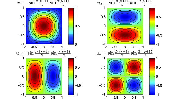
Figure 1: Four eigenfunctions of problem (2.14): $u_{1}$ keeps invariant under $\{E,\sigma_{x},\sigma_{y},I\}$ and satisfies equation (2.15), and $u_{2}$, $u_{3}$ and $u_{4}$ satisfy (2.18), (2.16) and (2.17), respectively.

Under the assumption that all symmetries of the eigenvalue problem are included in group $G$ and no accidental degeneracy occurs, the eigenvalue degeneracy is determined by the dimensionalities of irreducible representations of $G$ [47, 52]. For example, in cubic crystals all eigenstates have degeneracy 1, 2, or 3 [38]. According to Theorem 2.1 or Corollary 2.2, eigenvalues of each subproblem should be nondegenerate. In practice, we usually use part of symmetry operations. Thus subproblems will probably still have degenerate eigenvalues. However, it is possible to improve the spectral separation, especially when we exploit as many symmetries as possible. This would benefit the convergence of iterative diagonalization.

Formulation (2.13) makes a straightforward implementation for grid-based discretizations. We shall discuss the way to solve the subproblems in the next section.

3 Discretization

In this section, we study the discretized eigenvalue problems for subproblems (2.11) and (2.13). First we deduce our discretized systems when grid-based discretizations are employed. Then we provide a construction procedure for the symmetry-adapted bases, based on which we illustrate the relation of our discretized systems to those formed by symmetry-adapted bases.

Note that the $d_{\nu}$ subproblems associated with different $\nu$ values are independent and have the same formulation. So we take one $\nu\in\{1,2,\ldots,n_{c}\}$ and discuss the corresponding $d_{\nu}$ subproblems.

3.1 Our discretized system

Suppose $\Omega$ is discretized by a symmetrical grid with respect to group $G$, and $N$ is the number of degrees of freedom. For simplicity we assume that no degree of freedom lies on symmetry elements .

We determine a smallest set of degrees of freedom that could produce all $N$ ones by applying symmetry operations $\{R\in G\}$. It is clear that the number of degrees of freedom in this smallest set satisfies $N_{0}=\frac{1}{g}N$. We denote the set as

$$\{x_{j}:j=1,2,\ldots,N_{0}\},$$

then all degrees of freedom can be given by

$$\{R(j):j=1,2,\ldots,N_{0},~{}R\in G\},$$

where $R(j)\equiv Rx_{j}~{}(j=1,2,\ldots,N_{0})$.

The symmetry characteristic equation in (2.13) tells that for any $l\in\{1,2,\ldots,d_{\nu}\}$, the values of $u_{l}^{(\nu)}$ on all degrees of freedom $\{R(j):j=1,2,\ldots,N_{0},~{}R\in G\}$ are determined by the values of $\{u_{1}^{(\nu)},\ldots,u_{d_{\nu}}^{(\nu)}\}$ on $\{j:j=1,2,\ldots,N_{0}\}$. Thus, the size of discretized eigenvalue problem for (2.13) is $d_{\nu}N_{0}$.

If the given irreducible representation $\Gamma^{(\nu)}$ is one-dimensional, then (2.13) gives

$$\left\{\begin{array}[]{rcll}Lu^{(\nu)}&=&\lambda^{(\nu)}u^{(\nu)}&\quad\mbox{in}~{}\Omega,\\ u^{(\nu)}&=&0&\quad\mbox{on}~{}\partial\Omega,\\ u^{(\nu)}(Rx)&=&{\Gamma^{(\nu)}(R)}^{*}~{}u^{(\nu)}(x)&\quad\mbox{in}~{}\Omega,~{}\forall R\in G,\end{array}\right.$$ (3.1)

where we omit subscripts of ${\Gamma^{(\nu)}(R)}^{*}_{11}$ and $u_{1}^{(\nu)}$.

Suppose the discretized system for eigenvalue problem (3.1) is

$$\sum_{j=1}^{N_{0}}\sum_{R\in G}a_{\scriptscriptstyle{i,R(j)}}u_{\scriptscriptstyle{R(j)}}=\lambda\sum_{j=1}^{N_{0}}\sum_{R\in G}b_{\scriptscriptstyle{i,R(j)}}u_{\scriptscriptstyle{R(j)}},\quad i=1,2,\ldots,N_{0},$$

where $u_{\scriptscriptstyle{R(j)}}$ is the unknown associated with $Rx_{j}$ and $\{a_{\scriptscriptstyle{i,R(j)}},b_{\scriptscriptstyle{i,R(j)}}\}$ represent the discretization coefficients. For instance, in finite element discretizations, $a_{\scriptscriptstyle{i,R(j)}}$ and $b_{\scriptscriptstyle{i,R(j)}}$ are entries of the stiffness and mass matrices, respectively. Note that for any $i\in\{1,2,\ldots,N_{0}\}$, although the discretization equation seems to involve all $N$ degrees of freedom $\{R(j):j=1,2,\ldots,N_{0},~{}R\in G\}$, in fact only part of coefficients $\{a_{\scriptscriptstyle{i,R(j)}},~{}b_{\scriptscriptstyle{i,R(j)}}:j=1,2,\ldots,N_{0},~{}R\in G\}$ are non-zero. An extreme example is that in finite difference discretizations $b_{\scriptscriptstyle{i,R(j)}}=\delta_{\scriptscriptstyle{i,R(j)}}~{}(j=1,2,\ldots,N_{0},~{}R\in G)$ for any $i\in\{1,2,\ldots,N_{0}\}$.

We know from the symmetry characteristic equation that the discretized system is then reduced to

$$\sum_{j=1}^{N_{0}}\sum_{R\in G}{\Gamma^{(\nu)}(R)}^{*}~{}a_{\scriptscriptstyle{i,R(j)}}~{}u_{\scriptscriptstyle{j}}=\lambda\sum_{j=1}^{N_{0}}\sum_{R\in G}{\Gamma^{(\nu)}(R)}^{*}~{}b_{\scriptscriptstyle{i,R(j)}}~{}u_{\scriptscriptstyle{j}},\quad i=1,2,\ldots,N_{0}.$$

Denote the solution vector as

$${\bf u}=(u_{1},u_{2},\ldots,u_{N_{0}})^{\mathsf{T}},$$

we may rewrite the discretized system as a matrix form

$$A{\bf u}=\lambda B{\bf u},$$

where

$$\begin{array}[]{rcll}A&=&(A_{ij})_{N_{0}\times N_{0}},&~{}A_{ij}={\displaystyle\sum_{R\in G}}{\Gamma^{(\nu)}(R)}^{*}~{}a_{\scriptscriptstyle{i,R(j)}},\vspace{0.1cm}\\ B&=&(B_{ij})_{N_{0}\times N_{0}},&~{}B_{ij}={\displaystyle\sum_{R\in G}}{\Gamma^{(\nu)}(R)}^{*}~{}b_{\scriptscriptstyle{i,R(j)}}.\end{array}$$ (3.2)

In the case of higher-dimensional irreducible representations, the $d_{\nu}$ subproblems in (2.13) are coupled through symmetry characteristics. Taking $d_{\nu}=2$ as an example, we assemble subproblems for $u_{1}^{(\nu)}$ and $u_{2}^{(\nu)}$ in (2.13) to solve eigenvalue problem

$$\quad\left\{\begin{array}[]{rcll}\left[\begin{array}[]{c}Lu_{1}^{(\nu)}\vspace{0.1cm}\\ Lu_{2}^{(\nu)}\end{array}\right]&=&\lambda^{(\nu)}\left[\begin{array}[]{c}u_{1}^{(\nu)}\vspace{0.1cm}\\ u_{2}^{(\nu)}\end{array}\right]&\mbox{in}~{}\Omega,\vspace{0.2cm}\\ \left[\begin{array}[]{c}u_{1}^{(\nu)}\vspace{0.1cm}\\ u_{2}^{(\nu)}\end{array}\right](Rx)&=&\left[\begin{array}[]{cc}{\Gamma^{(\nu)}(R)}^{*}_{11}&{\Gamma^{(\nu)}(R)}^{*}_{12}\vspace{0.1cm}\\ {\Gamma^{(\nu)}(R)}^{*}_{21}&{\Gamma^{(\nu)}(R)}^{*}_{22}\\ \end{array}\right]\left[\begin{array}[]{c}u_{1}^{(\nu)}\vspace{0.1cm}\\ u_{2}^{(\nu)}\end{array}\right](x)&\mbox{in}~{}\Omega,~{}\forall R\in G,\vspace{0.2cm}\\ \left[\begin{array}[]{c}u_{1}^{(\nu)}\vspace{0.1cm}\\ u_{2}^{(\nu)}\end{array}\right]&=&\left[\begin{array}[]{c}0\vspace{0.1cm}\\ 0\end{array}\right]&\mbox{on}~{}\partial\Omega.\end{array}\right.$$ (3.3)

Suppose the discretized system associated with (3.3) is

$$\left\{\begin{array}[]{c}{\displaystyle\sum_{j=1}^{N_{0}}\sum_{R\in G}}~{}a_{\scriptscriptstyle{i,R(j)}}~{}u_{\scriptscriptstyle{1,R(j)}}=\lambda~{}{\displaystyle\sum_{j=1}^{N_{0}}\sum_{R\in G}}~{}b_{\scriptscriptstyle{i,R(j)}}~{}u_{\scriptscriptstyle{1,R(j)}},\quad i=1,2,\ldots,N_{0},\vspace{0.1cm}\\ {\displaystyle\sum_{j=1}^{N_{0}}\sum_{R\in G}}~{}a_{\scriptscriptstyle{i,R(j)}}~{}u_{\scriptscriptstyle{2,R(j)}}=\lambda~{}{\displaystyle\sum_{j=1}^{N_{0}}\sum_{R\in G}}~{}b_{\scriptscriptstyle{i,R(j)}}~{}u_{\scriptscriptstyle{2,R(j)}},\quad i=1,2,\ldots,N_{0},\end{array}\right.$$

where $u_{\scriptscriptstyle{1,R(j)}}$ and $u_{\scriptscriptstyle{2,R(j)}}$ are the unknowns associated with $Rx_{j}$. Denote the solution vector as

$${\bf v}=(u_{11},u_{12},\ldots,u_{1N_{0}},~{}u_{21},u_{22},\ldots,u_{2N_{0}})^{\mathsf{T}}$$

and rewrite the discretized system as a matrix form

$$A{\bf v}=\lambda B{\bf v}.$$

We have

$$A=\left[\begin{array}[]{cc}A_{[11]}&A_{[12]}\\ A_{[21]}&A_{[22]}\end{array}\right],~{}B=\left[\begin{array}[]{cc}B_{[11]}&B_{[12]}\\ B_{[21]}&B_{[22]}\end{array}\right],$$

where $A_{[ml]}=(A_{[ml]ij})_{N_{0}\times N_{0}}~{}(m,l=1,2)$ with

$$\begin{array}[]{rcll}A_{[11]ij}&=&{\displaystyle\sum_{R\in G}}{\Gamma^{(\nu)}(R)}^{*}_{11}~{}a_{\scriptscriptstyle{i,R(j)}},&~{}A_{[12]ij}={\displaystyle\sum_{R\in G}}{\Gamma^{(\nu)}(R)}^{*}_{12}~{}a_{\scriptscriptstyle{i,R(j)}},\vspace{0.1cm}\\ A_{[21]ij}&=&{\displaystyle\sum_{R\in G}}{\Gamma^{(\nu)}(R)}^{*}_{21}~{}a_{\scriptscriptstyle{i,R(j)}},&~{}A_{[22]ij}={\displaystyle\sum_{R\in G}}{\Gamma^{(\nu)}(R)}^{*}_{22}~{}a_{\scriptscriptstyle{i,R(j)}}.\end{array}$$ (3.4)

Entries of $B$ are in the same form as those of $A$ and can be obtained by substituting $a_{\scriptscriptstyle{i,R(j)}}$ with $b_{\scriptscriptstyle{i,R(j)}}$.

If symmetry group $G$ is Abelian, each irreducible representation is one-dimensional and all discretized subproblems are independent. Otherwise, there exist $\Gamma^{(\nu)}$ with $d_{\nu}>1$ and the corresponding $d_{\nu}$ discretized subproblems are coupled through symmetry characteristics. Thus, no matter $G$ is Abelian or not, we shall solve $n_{c}$ decoupled eigenvalue problems, where $n_{c}$ is the number of irreducible representations. And the size of discretized system for the $\nu$-th problem is $d_{\nu}N_{0}$.

3.2 Symmetry-adapted bases

In Section 3.3, we shall illustrate the relation between our approach and the approach that constructs symmetry-adapted bases. For this purpose, in the current subsection, we tell how to construct the symmetry-adapted bases, which is the most critical step in the latter approach.

Consider the weak form of (2.10): find $(\lambda,u)\in\mathbb{R}\times V$ such that

$$a(u,v)=\lambda(u,v)\quad\forall v\in V,$$

where $a(\cdot,\cdot)$ is the associated bilinear form over $V\times V$.

Note that the discussion in this part is not restricted to grid-based discretizations, but we still use notation $N$ and $N_{0}$ for brevity. Suppose that we start from $N$ basis functions $\{\psi\}$ of some type, which satisfy that for any $R\in G$, $P_{R}\psi$ is one of the basis functions when $\psi$ is, i.e., the $N$ basis functions are chosen with respect to symmetry group $G$. For simplicity, like the assumption for grid-based discretizations, we assume that the $g$ basis functions $\{P_{R}\psi:R\in G\}$ are linearly independent for any basis function $\psi$. We see that the number of basis functions in the set which could produce all $N$ ones by applying $\{R\in G\}$ is $g$ times smaller than $N$. We denote this set by

$$\{\psi_{j}:j=1,2,\ldots,N_{0}\},$$

then all basis functions are given as

$$\{P_{R}\psi_{j}:j=1,2,\ldots,N_{0},~{}R\in G\}.$$

For the given $\nu$, we fix some $k\in\{1,2,\ldots,d_{\nu}\}$ and generate symmetry-adapted bases for the $k$-th subproblem in (2.11). This is achieved by applying projection operator $\mathscr{P}^{(\nu)}_{kk}$ on all the basis functions $\{P_{R}\psi_{j}:j=1,2,\ldots,N_{0},~{}R\in G\}$. Suppose that we obtain $N^{\prime}$ linearly independent symmetry-adapted bases from this process and we denote them as $\{\Psi_{j}:j=1,2,\ldots,N^{\prime}\}$. Then for any $l\in\{1,2,\ldots,d_{\nu}\}$, symmetry-adapted bases for the $l$-th subproblem can be given as $\{\mathscr{P}^{(\nu)}_{lk}\Psi_{j}:j=1,2,\ldots,N^{\prime}\}$.

Consider the $d_{\nu}$ discretized systems under the generated bases. Matrix elements of the $l$-th discretized system are

$$a(\mathscr{P}^{(\nu)}_{lk}\Psi_{j},\mathscr{P}^{(\nu)}_{lk}\Psi_{i}),~{}(\mathscr{P}^{(\nu)}_{lk}\Psi_{j},\mathscr{P}^{(\nu)}_{lk}\Psi_{i}),\quad i,j=1,2,\ldots,N^{\prime}.$$

For each $j\in\{1,2,\ldots,N^{\prime}\}$, according to Proposition 2.1, $\{\mathscr{P}^{(\nu)}_{lk}\Psi_{j}:l=1,2,\ldots,d_{\nu}\}$ form a basis for $\Gamma^{(\nu)}$. We see from (2.3) and Proposition 2.3 that all the $d_{\nu}$ discretized systems are the same. So we only need to solve the discretized system corresponding to the $k$-th subproblem:

$$\sum_{j=1}^{N^{\prime}}a(\Psi_{j},\Psi_{i})~{}\alpha_{j}=\lambda^{(\nu)}\sum_{j=1}^{N^{\prime}}(\Psi_{j},\Psi_{i})~{}\alpha_{j},\quad i=1,2,\ldots,N^{\prime},$$

where $\{\alpha_{j}\}$ are the unknowns. After calculating $\{\alpha_{j}\}$, the approximated eigenfunctions for the $l$-th subproblem can be achieved by

$$u_{l}^{(\nu)}=\sum_{j=1}^{N^{\prime}}\alpha_{j}\mathscr{P}^{(\nu)}_{lk}\Psi_{j},\quad l=1,2,\ldots,d_{\nu}.$$

Next we show how many symmetry-adapted bases would be constructed for the $\nu$-$k$ symmetry, i.e., the number $N^{\prime}$ of linearly independent symmetry-adapted functions in

$$\mathscr{P}^{(\nu)}_{kk}\{P_{R}\psi_{j}:j=1,2,\ldots,N_{0},~{}R\in G\}.$$

And then we give the specific way to obtain these functions.

Theorem 3.1.

Suppose the original basis functions $\{P_{R}\psi_{j}:j=1,2,\ldots,N_{0},~{}R\in G\}$ satisfy that for each $j\in\{1,2,\ldots,N_{0}\}$ the $g$ functions in $\{P_{R}\psi_{j}:R\in G\}$ are linearly independent. Then for any given $\nu\in\{1,2,\ldots,n_{c}\}$ and $k\in\{1,2,\ldots,d_{\nu}\}$, there are $d_{\nu}N_{0}$ symmetry-adapted bases for the $\nu$-$k$ symmetry.

Proof.

We need to prove that there are exactly $d_{\nu}N_{0}$ linearly independent symmetry-adapted functions in $\{\mathscr{P}^{(\nu)}_{kk}P_{R}\psi_{j}:j=1,2,\ldots,N_{0},~{}R\in G\}$.

For any $R\in G$ and $j\in\{1,2,\ldots,N_{0}\}$, since

$$\mathscr{P}^{(\nu)}_{kk}P_{R}\psi_{j}=\frac{d_{\nu}}{g}\sum_{R^{\prime}\in G}{\Gamma^{(\nu)}(R^{\prime})}^{*}_{kk}P_{R^{\prime}}P_{R}\psi_{j}=\frac{d_{\nu}}{g}\sum_{S\in G}{\Gamma^{(\nu)}(SR^{-1})}^{*}_{kk}P_{S}\psi_{j},$$ (3.5)

we see that $\mathscr{P}^{(\nu)}_{kk}P_{R}\psi_{j}$ is a linear combination of functions $\{P_{S}\psi_{j}:S\in G\}$ and the coefficient of $P_{S}\psi_{j}$ is $\frac{d_{\nu}}{g}{\Gamma^{(\nu)}(SR^{-1})}^{*}_{kk}$. Obviously, functions in $\{\mathscr{P}^{(\nu)}_{kk}P_{R}\psi_{j}:j=1,2,\ldots,N_{0},~{}R\in G\}$ with different $j$ values are linearly independent. So we only need to determine the number of symmetry-adapted bases in $\{\mathscr{P}^{(\nu)}_{kk}P_{R}\psi_{j}:R\in G\}$ for any given $j\in\{1,2,\ldots,N_{0}\}$.

Since $\{P_{S}\psi_{j}:S\in G\}$ are linearly independent and $R^{-1}$ runs over all elements of group $G$ when $R$ does, (3.5) tells that the number of linearly independent functions in $\{\mathscr{P}^{(\nu)}_{kk}P_{R}\psi_{j}:R\in G\}$ equals to the rank of matrix $C=(C_{mn})_{g\times g}$, where $C_{mn}={\Gamma^{(\nu)}(R_{m}R_{n})}^{*}_{kk}.$

We observe that $C$ can be written as

$$C=\left[\begin{array}[]{ccc}{\Gamma^{(\nu)}(R_{1})}^{*}_{k1}&\ldots&{\Gamma^{(\nu)}(R_{1})}^{*}_{kd_{\nu}}\\ {\Gamma^{(\nu)}(R_{2})}^{*}_{k1}&\ldots&{\Gamma^{(\nu)}(R_{2})}^{*}_{kd_{\nu}}\\ \vdots&&\vdots\\ {\Gamma^{(\nu)}(R_{g})}^{*}_{k1}&\ldots&{\Gamma^{(\nu)}(R_{g})}^{*}_{kd_{\nu}}\end{array}\right]\left[\begin{array}[]{ccc}{\Gamma^{(\nu)}(R_{1})}^{*}_{1k}&\ldots&{\Gamma^{(\nu)}(R_{g})}^{*}_{1k}\\ {\Gamma^{(\nu)}(R_{1})}^{*}_{2k}&\ldots&{\Gamma^{(\nu)}(R_{g})}^{*}_{2k}\\ \vdots&&\vdots\\ {\Gamma^{(\nu)}(R_{1})}^{*}_{d_{\nu}k}&\ldots&{\Gamma^{(\nu)}(R_{g})}^{*}_{d_{\nu}k}\end{array}\right]\equiv C_{1}C_{2},$$

where $C_{1}$ and $C_{2}$ are $g\times d_{\nu}$ and $d_{\nu}\times g$ matrices, respectively. We obtain from the great orthogonality theorem (2.1) that columns of $C_{1}$ are orthogonal, and so are rows of $C_{2}$, i.e.,

$$\mbox{rank}(C_{1})=\mbox{rank}(C_{2})=d_{\nu}.$$

Thus

$$\mbox{rank}(C)=\mbox{rank}(C_{1}C_{2})=d_{\nu},$$

and we completed the proof.   ∎

Remark 3.1.

For the given $\nu$ and $k$, Theorem 3.1 indicates that there are $d_{\nu}$ symmetry-adapted bases for each $j\in\{1,2,\ldots,N_{0}\}$. It remains a problem how to obtain these $d_{\nu}$ functions. We see from (3.5) that, whenever the chosen $d_{\nu}$ operations $\{R_{n}\in G:n=1,2,\ldots,d_{\nu}\}$ satisfy that the $k$-th columns of matrices $\{\Gamma^{(\nu)}(R_{n}^{-1}):n=1,2,\ldots,d_{\nu}\}$ are linearly independent, $\{\mathscr{P}^{(\nu)}_{kk}P_{R_{n}}\psi_{j}:n=1,2,\ldots,d_{\nu}\}$ exactly give the $d_{\nu}$ symmetry-adapted bases.

3.3 Relation

In this part, taking the finite element discretization as an example, we investigate the relation between our discretized systems and those formed by the symmetry-adapted bases.

Consider the finite element discretization and denote the basis function corresponding to any $j\in\{1,2,\ldots,N_{0}\}$ as $\varphi_{j}$. We see from $P_{R}\varphi_{j}(x)=\varphi_{j}(R^{-1}x)$ that $P_{R}\varphi_{j}$ is the basis function corresponding to $R(j)$, i.e.,

$$P_{R}\varphi_{j}=\varphi_{\scriptscriptstyle{R(j)}}.$$

Our discretized systems associated with the finite element basis functions $\{P_{R}\varphi_{j}:j=1,2,\ldots,N_{0},~{}R\in G\}$ are determined by setting $a_{\scriptscriptstyle{i,R(j)}}$ and $b_{\scriptscriptstyle{i,R(j)}}$ in (3.2) and (3.4) as

$$a_{\scriptscriptstyle{i,R(j)}}=a(P_{R}\varphi_{j},\varphi_{i}),\quad b_{\scriptscriptstyle{i,R(j)}}=(P_{R}\varphi_{j},\varphi_{i}).$$ (3.6)

Now we turn to study the discretized systems from the approach that constructs symmetry-adapted bases, and obtain the relation between the two approaches.

In the case of $d_{\nu}=1$, we apply projection operator $\mathscr{P}^{(\nu)}$ on all the finite element basis functions to construct the symmetry-adapted bases. We see from Theorem 3.1 that for each $j\in\{1,2,\ldots,N_{0}\}$, $\{\mathscr{P}^{(\nu)}P_{R}\varphi_{j}:R\in G\}$ give one symmetry-adapted basis function. According to Remark 3.1, we can choose $R=E$ to get all the $N_{0}$ symmetry-adapted bases as follows

$$\Phi_{j}=\mathscr{P}^{(\nu)}\varphi_{j},~{}j=1,2,\ldots,N_{0}.$$

The discretized system under these bases then becomes

$$\sum_{j=1}^{N_{0}}a(\Phi_{j},\Phi_{i})c_{j}=\tilde{\lambda}\sum_{j=1}^{N_{0}}(\Phi_{j},\Phi_{i})c_{j},\quad i=1,2,\ldots,N_{0},$$

where $\{c_{j}\}$ are the unknowns. Equivalently,

$$\widetilde{A}\tilde{\bf u}=\tilde{\lambda}\widetilde{B}\tilde{\bf u},$$

where $\tilde{\bf u}=(c_{1},c_{2},\ldots,c_{N_{0}})^{\mathsf{T}}$ and

$$\begin{array}[]{rcll}\widetilde{A}&=&(\widetilde{A}_{ij})_{N_{0}\times N_{0}},&~{}\widetilde{A}_{ij}=\frac{1}{g}{\displaystyle\sum_{R\in G}}{\Gamma^{(\nu)}(R)}^{*}~{}a(P_{R}\varphi_{j},\varphi_{i}),\vspace{0.1cm}\\ \widetilde{B}&=&(\widetilde{B}_{ij})_{N_{0}\times N_{0}},&~{}\widetilde{B}_{ij}=\frac{1}{g}{\displaystyle\sum_{R\in G}}{\Gamma^{(\nu)}(R)}^{*}(P_{R}\varphi_{j},\varphi_{i}).\end{array}$$ (3.7)

Comparing (3.7) with (3.2) and using (3.6), we obtain

$$\widetilde{A}=\frac{1}{g}A,~{}\widetilde{B}=\frac{1}{g}B.$$

Thus, in the case of $d_{\nu}=1$, there holds

$$\lambda=\tilde{\lambda},~{}{\bf u}=\tilde{\bf u}.$$

In the case of $d_{\nu}=2$, there are two subproblems in (2.11). We choose $k=1$ and apply projection operator $\mathscr{P}^{(\nu)}_{11}$ on all the finite element basis functions to construct symmetry-adapted bases for the first subproblem. Theorem 3.1 tells that for each $j\in\{1,2,\ldots,N_{0}\}$, $\{\mathscr{P}^{(\nu)}_{11}P_{R}\varphi_{j}:R\in G\}$ give $d_{\nu}=2$ symmetry-adapted bases. According to Remark 3.1, we choose identity operation $E$ and another $S\in G$ which satisfy that the first columns of matrices $\{\Gamma^{(\nu)}(E),~{}\Gamma^{(\nu)}(S^{-1})\}$ are linearly independent. Then

$$\{\mathscr{P}^{(\nu)}_{11}\varphi_{j},\mathscr{P}^{(\nu)}_{11}P_{S}\varphi_{j}:j=1,2,\ldots,N_{0}\}$$

give all the $2N_{0}$ bases adapted to the $\nu$-$1$ symmetry as follows

$$(\Phi_{1},\ldots,\Phi_{N_{0}},\Psi_{1},\ldots,\Psi_{N_{0}})=(\mathscr{P}^{(\nu)}_{11}\varphi_{1},\ldots,\mathscr{P}^{(\nu)}_{11}\varphi_{N_{0}},\mathscr{P}^{(\nu)}_{11}P_{S}\varphi_{1},\ldots,\mathscr{P}^{(\nu)}_{11}P_{S}\varphi_{N_{0}}).$$

The discretized system under these bases is

$$\left\{\begin{array}[]{c}{\displaystyle\sum_{j=1}^{N_{0}}}~{}a(c_{1j}\Phi_{j}+c_{2j}\Psi_{j},\Phi_{i})=\tilde{\lambda}~{}{\displaystyle\sum_{j=1}^{N_{0}}}~{}(c_{1j}\Phi_{j}+c_{2j}\Psi_{j},\Phi_{i}),\quad i=1,2,\ldots,N_{0},\vspace{0.1cm}\\ {\displaystyle\sum_{j=1}^{N_{0}}}~{}a(c_{1j}\Phi_{j}+c_{2j}\Psi_{j},\Psi_{i})=\tilde{\lambda}~{}{\displaystyle\sum_{j=1}^{N_{0}}}~{}(c_{1j}\Phi_{j}+c_{2j}\Psi_{j},\Psi_{i}),\quad i=1,2,\ldots,N_{0},\end{array}\right.$$

where $\{c_{1j},c_{2j}\}$ represent the unknowns. Equivalently,

$$\widetilde{A}\tilde{\bf v}=\tilde{\lambda}\widetilde{B}\tilde{\bf v},$$

where $\tilde{\bf v}=(c_{11},c_{12},\ldots,c_{1N_{0}},~{}c_{21},c_{22},\ldots,c_{2N_{0}})^{\mathsf{T}}$ and

$$\widetilde{A}=\left[\begin{array}[]{cc}\widetilde{A}_{[11]}&\widetilde{A}_{[12]}\vspace{0.1cm}\\ \widetilde{A}_{[21]}&\widetilde{A}_{[22]}\end{array}\right],~{}\widetilde{B}=\left[\begin{array}[]{cc}\widetilde{B}_{[11]}&\widetilde{B}_{[12]}\vspace{0.1cm}\\ \widetilde{B}_{[21]}&\widetilde{B}_{[22]}\end{array}\right].$$

A simple calculation shows

$$\widetilde{A}_{[11]} = \frac{2}{g}A_{[11]},$$

$$\widetilde{A}_{[12]} = \frac{2}{g}\left(\Gamma^{(\nu)}(S)_{11}A_{[11]}+\Gamma^{(\nu)}(S)_{12}A_{[12]}\right),$$

$$\widetilde{A}_{[21]} = \frac{2}{g}\left({\Gamma^{(\nu)}(S)}^{*}_{11}A_{[11]}+{\Gamma^{(\nu)}(S)}^{*}_{12}A_{[21]}\right),$$

$$\widetilde{A}_{[22]} = \frac{2}{g}\Big{\{}{\Gamma^{(\nu)}(S)}_{11}\left({\Gamma^{(\nu)}(S)}^{*}_{11}A_{[11]}+{\Gamma^{(\nu)}(S)}^{*}_{12}A_{[21]}\right)$$

$$+~{}{\Gamma^{(\nu)}(S)}_{12}\left({\Gamma^{(\nu)}(S)}^{*}_{11}A_{[12]}+{\Gamma^{(\nu)}(S)}^{*}_{12}A_{[22]}\right)\Big{\}}.$$

Let

$$Q_{l}=\left[\begin{array}[]{cc}I_{N_{0}\times N_{0}}&{\bf 0}_{N_{0}\times N_{0}}\vspace{0.2cm}\\ {\Gamma^{(\nu)}(S)}^{*}_{11}I_{N_{0}\times N_{0}}&{\Gamma^{(\nu)}(S)}^{*}_{12}I_{N_{0}\times N_{0}}\end{array}\right],~{}Q_{r}=\left[\begin{array}[]{cc}I_{N_{0}\times N_{0}}&\Gamma^{(\nu)}(S)_{11}I_{N_{0}\times N_{0}}\vspace{0.2cm}\\ {\bf 0}_{N_{0}\times N_{0}}&\Gamma^{(\nu)}(S)_{12}I_{N_{0}\times N_{0}}\end{array}\right],$$

we have

$$Q_{l}AQ_{r}=\frac{g}{2}\widetilde{A}.$$

Similarly

$$Q_{l}BQ_{r}=\frac{g}{2}\widetilde{B}.$$

Thus, in the case of $d_{\nu}=2$, we get

$$\lambda=\tilde{\lambda},\quad{\bf v}=Q_{r}\tilde{\bf v},$$

i.e.,

$$u_{1j}=c_{1j}+{\Gamma^{(\nu)}(S)}_{11}c_{2j},~{}u_{2j}={\Gamma^{(\nu)}(S)}_{12}c_{2j},\quad j=1,2,\ldots,N_{0}.$$

Consider a given $\nu\in\{1,2,\ldots,n_{c}\}$, the approach that constructs symmetry-adapted bases seems to have an obvious advantage that the $d_{\nu}$ subproblems are decoupled. Theorem 3.1 tells that the number of symmetry-adapted bases for each subproblem is in fact $d_{\nu}N_{0}$. Therefore, the coupled eigenvalue problem appeared in our decomposition approach is not an induced complexity, but some reflection of the intrinsic property of symmetry-based decomposition.

Solving subproblems instead of the original eigenvalue problem shall reduce the computational overhead and memory requirement to a large extent. The eigenvalues to be computed are distributed among subproblems, i.e., a smaller number of eigenpairs are required for each subproblem. And the decomposed problems can be solved in a small subdomain. Moreover, as indicated in Section 2, there is a possibility to improve the spectral separation, which would accelerate convergence of iterative diagonalization. In the next section, we shall propose a way to analyze the practical decrease in the computational cost.

4 Complexity and performance analysis

The advantage of solving subproblems (2.13) instead of the original problem (2.10) is the reduction in computational overhead. Based on a complexity analysis, we quantize this reduction and present a way to analyze the practical speedup in CPU time.

4.1 Complexity analysis

Computational complexity is the dominant part of computational overhead when the size of problem becomes sufficiently large. So the fundamental step of complexity analysis is to figure out the computational cost in floating point operations (flops).

In our computation, the algebraic eigenvalue problem will be solved by the implicitly restarted Lanczos method (IRLM) implemented in ARPACK package [37]. Our complexity analysis will be based on IRLM, whereas it can be extended to other iterative diagonalization methods.

Total flops of an iterative method are the product of the number of iteration steps and the number of flops per iteration. We shall analyze the number of flops per iteration, for which purpose we represent the procedure of IRLM as Algorithm 4.1 as follows.

Input: Maximum number of iteration steps; The $m$-step Lanczos Factorization $AV_{m}=V_{m}H_{m}+f_{m}e_{m}^{T}$.

1

2repeat

3       Compute the Schur decomposition of symmetric tridiagonal matrix $H_{m}$ and select the set of $l$ shifts $\mu_{1},\mu_{2},\dots,\mu_{l}$;

4      

5      $q^{T}\leftarrow e^{T}_{m}$;

6      

7      for $j=1,2,\dots,l$ do

8            

9            $H_{m}-\mu_{j}I=Q_{j}R_{j}$, $H_{m}\leftarrow R_{j}Q_{j}+\mu_{j}I$;

10            

11            $V_{m}\leftarrow V_{m}Q_{j}$, $q^{H}\leftarrow q^{H}Q_{j}$;

12            

13       end for

14      

15      $f_{k}\leftarrow v_{k+1}\hat{\beta}_{k}+f_{m}\sigma_{k},V_{k}\leftarrow V_{m}(1:n,1:k),H_{k}\leftarrow H_{m}(1:k,1:k)$;

16      

17      Beginning with the $k$-step Lanczos factorization $AV_{k}=V_{k}H_{k}+f_{k}e_{k}^{T}$, apply $l$ additional steps of the Lanczos process to obtain a new $m$-step Lanczos factorization $AV_{m}=V_{m}H_{m}+f_{m}e_{m}^{T}$;

18      

19until Convergence or the number of iteration steps exceeded the maximum one;

Algorithm 4.1 An implicitly restarted Lanczos method

Table 2: Notation in Algorithm 4.1.

Notation	Description
$m$	the maximum dimension of the Krylov subspace,
	twice the number of required eigenpairs plus 5 in our computation
$l$	the number of Lanczos factorization steps, s.t. $m=k+l$
$A$	the (sparse) matrix size of $n\times n$,
	arising from the grid-based discretization of (2.10) or (2.13)
$V_{m}$	the matrix size of $n\times m$,
	made of $m$ column vectors as the basis of the Krylov subspace
$H_{m}$	the symmetric tridiagonal matrix size of $m\times m$
$f_{m}$	the column vector size of $n$,
	the residual vector after $m$ steps of Lanczos factorization
$e_{m}$	the unit column vector size of $m$, in which the $m$-th component is one
$R_{j}$	the upper triangular matrix size of $m\times m$
$Q_{j}$	the unitary matrix size of $m\times m$
$v_{k+1}$	the $(k+1)$-th column vector of $V_{m}$
$\hat{\beta}_{k}$	$H_{m}(k+1,k)$
$\sigma_{k}$	the $k$-th component of vector $q$

Table 2 is a supplementary remark to Algorithm 4.1. In Algorithm 4.1, Step 2 is the Schur decomposition of $H_{m}$, and consumes about $6m^{2}$ flops [24]. Steps 4 to 7 do $l$-step QR iteration with shifts. Note that each $Q_{j}$ is the product of $(m-1)$ Givens transformations, we have that Step 5 costs $8m(m-1)$ flops since applying one Givens transformation to a matrix only changes two rows or columns of the matrix. And for the same reason, Step 6 costs $4(m-1)(n+1)$ flops. Consequently Steps 4 to 7 consume $4l(m-1)(2m+n+1)$ flops. Regardless of BLAS-1 operations, we do $l$ matrix-vector multiplication operations at Step 9.

Besides order $n$ of the matrix, the flops of one matrix-vector multiplication also depend on the order of finite difference or finite elements. If the shift-invert mode in ARPACK is employed to solve the generalized eigenvalue problem arising from the finite element discretization, the matrix-vector multiplication will be realized by some iterative linear solver. So we cannot figure out accurately the flops per matrix-vector multiplication but represent it as $\mathcal{O}(n)$.

In total, the computational overhead per IRLM iteration can be estimated as

$$6m^{2}+l\left(4(m-1)(2m+n+1)+\mathcal{O}(n)\right)$$

flops. In general, order $n$ of the matrix is much more than $m$ for grid-based discretizations. So the majority of flops per IRLM iteration is

$$f(l,m,n)=l\left(4mn+\mathcal{O}(n)\right).$$ (4.1)

In order to make clear the reduction in flops per iteration from solving subproblems instead of the original eigenvalue problem, we divide the flops per iteration into two parts. One is required by $l$-step $QR$ iteration, and the other is spent on $l$ operations of matrix-vector multiplication. We denote them by $f_{1}$ and $f_{2}$ respectively and rewrite (4.1) as follows

$$f(l,m,n)=f_{1}(l,m,n)+f_{2}(l,m,n),$$ (4.2)

where $f_{1}(l,m,n)=4lmn$ and $f_{2}(l,m,n)=\mathcal{O}(ln)$.

In solving the original eigenvalue problem (2.10), the major flops per IRLM iteration can be accounted as (4.1) or (4.2) with $n=N$. In the decomposition approach, as discussed in Section 3.1, we shall solve $n_{c}$ decoupled eigenvalue problems, and the size of discretized system for the $\nu$-th problem is $d_{\nu}N_{0}$. In solving the $\nu$-th problem (2.13), $m$ is reduced to $m/\theta_{1}$, $N$ to $d_{\nu}N/g$, and $l$ to $l/\theta_{2}$, where $g$ is the order of finite group $G$, $\theta_{1}>1$ and $\theta_{2}\approx\theta_{1}$ because $l$ is almost proportional to $m$ in Algorithm 4.1. We shall explain in Section 5.2 that the number of required eigenpairs for each subproblem is set as the same in the computation, so all the subproblems have an identical $\theta_{1}$. Thus, the majority of total flops per iteration for all $n_{c}$ decomposed eigenvalue problems is

$$\sum_{\nu=1}^{n_{c}}f(\frac{l}{\theta_{2}},\frac{m}{\theta_{1}},\frac{d_{\nu}N}{g}) = \sum_{\nu=1}^{n_{c}}\left(f_{1}(\frac{l}{\theta_{2}},\frac{m}{\theta_{1}},\frac{d_{\nu}N}{g})+f_{2}(\frac{l}{\theta_{2}},\frac{m}{\theta_{1}},\frac{d_{\nu}N}{g})\right)$$ (4.3)

$$= \frac{n_{sub}}{g}\left(\frac{1}{\theta_{1}\theta_{2}}f_{1}(l,m,N)+\frac{1}{\theta_{2}}f_{2}(l,m,N)\right),$$

where $n_{sub}=\sum_{\nu=1}^{n_{c}}d_{\nu}$ is the number of subproblems.

As mentioned in Section 3, the decomposition approach saves the computational cost of solving the eigenvalue problem. Now the reduction can be characterized by (4.3).

4.2 Performance analysis

In (4.3), the order of factors for $f_{1}$ and $f_{2}$ differs, so the practical speedup in CPU time cannot be properly estimated from (4.3). We introduce the CPU time ratio $\omega$ of the matrix-vector multiplications to the whole IRLM process in solving the original eigenvalue problem (2.10). It is an a posteriori parameter which screens affects of implementation, the runtime environment, as well as the specific linear solver for the shift-invert mode. Besides, testing for $\omega$ is feasible as the operation of matrix-vector multiplication is usually provided by users.

Applying the symmetry-based decomposition approach instead of solving (2.10) directly, we can show the speedup in CPU time of one IRLM iteration as follows:

$$s(\theta_{1},\theta_{2},\omega)=\frac{\frac{1}{\omega}}{\frac{n_{sub}}{g}\left(\frac{1}{\theta_{1}\theta_{2}}\frac{1-\omega}{\omega}+\frac{1}{\theta_{2}}\right)}=\frac{g\theta_{1}\theta_{2}}{n_{sub}\left(1+(\theta_{1}-1)\omega\right)}.$$

That is

$$s(\theta_{1},\theta_{2},\omega)\approx\frac{g\theta_{1}^{2}}{n_{sub}\left(1+(\theta_{1}-1)\omega\right)}.$$ (4.4)

In practice, $\theta_{2}$ is actually determined by the internal configurations of algebraic eigenvalue solvers. So we prefer to use (4.4) to predict the CPU time speedup before solving subproblems (2.13).

In Section 6, the validation of (4.4) will be well supported by our numerical experiments. Moreover, this performance analysis implies that the speedup will be amplified when more eigenpairs are required and a consequent decrease in $\omega$ is very likely. Therefore, the symmetry-based decomposition will be attractive for large-scale eigenvalue problems.

5 Practical issues

In this section, we address some key issues in the implementation of the symmetry-based decomposition approach under grid-based discretizations.

5.1 Implementation of symmetry characteristics

Symmetry characteristics play a critical role in the decomposition approach, so it is important to preserve and realize symmetry characteristics for discretized eigenfunctions.

For all the degrees of freedom not lying on symmetry elements, the implementation of symmetry characteristics is straightforward with grid-based discretizations. If $x\in\Omega$ is a degree of freedom lying on the symmetry element corresponding to operation $R\in G$, the symmetry characteristic

$$u_{l}^{(\nu)}(Rx)=\sum_{m=1}^{d_{\nu}}{\Gamma^{(\nu)}(R)}^{*}_{lm}u_{m}^{(\nu)}(x)$$

reduces to

$$u_{l}^{(\nu)}(x)=\sum_{m=1}^{d_{\nu}}{\Gamma^{(\nu)}(R)}^{*}_{lm}u_{m}^{(\nu)}(x).$$

If $\mathrm{det}\left(\Gamma^{(\nu)}(R)-I_{d_{\nu}\times d_{\nu}}\right)\neq 0$, then all values $u_{1}^{(\nu)}(x),\dots,u_{d_{\nu}}^{(\nu)}(x)$ are zeros. Otherwise, we have to find the independent ones out of $u_{1}^{(\nu)}(x),\dots,u_{d_{\nu}}^{(\nu)}(x)$ and treat them as additional degrees of freedom.

In our computation, we discretize the problem on a tensor-product grid associated with the symmetry group. Currently, for simplicity, we use symmetry groups with symmetry elements on the coordinate planes, and prevent degrees of freedom from lying on the symmetry elements, by imposing an odd number of partition in each direction and using finite elements of odd orders.

5.2 Distribution of required eigenpairs among subproblems

The required eigenpairs of the original eigenvalue problem (2.10) are distributed among associated subproblems, and the number of eigenpairs required by each subproblem can be almost reduced by as many times as the number of subproblems. However, we are not able to see in advance the symmetry properties of eigenfunctions corresponding to required eigenvalues. Thus we have to consider some redundant eigenvalues for each subproblem.

We suppose to solve the first $N_{e}$ smallest eigenvalues of the original problem. First we set the number of eigenvalues to be computed for each subproblem as $\frac{N_{e}}{n_{sub}}$ plus redundant $n_{a}$ eigenvalues, where $n_{sub}=\sum_{\nu=1}^{n_{c}}d_{\nu}$ is the number of subproblems. After solving the subproblems, we gather eigenvalues from all subproblems and sort them in the ascending order. After taking $N_{e}$ smallest eigenvalues, we check which subproblems the remaining eigenvalues belong to. If there is no eigenvalue left for some subproblem, the number of computed eigenvalues for this subproblem is probably not enough. Subsequently we restart computing the subproblem with an increased number of required eigenpairs.

5.3 Two-level parallel implementation

We have addressed in Section 3 that the $n_{c}$ decomposed problems are independent to each other and can be solved simultaneously. Accordingly we have a two-level parallel implementation illustrated by Figure 2. At the first level, we dispatch the $n_{c}$ decomposed problems among groups of processors. At the second level, we distribute the grids among each group of processors. Since eigenfunctions of different subproblems are naturally orthogonal, there is no communication between different groups of processors during solving the eigenvalue problem. Such two-level or multi-level parallelism is likely appreciable for the architecture hierarchy of modern supercomputers. We shall see in Section 6.3 that the two-level parallel implementation does reduce the communication cost.

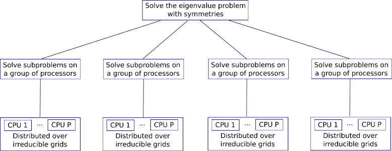
Figure 2: Schematic illustration of two-level parallel implementation for solving the eigenvalue problem with symmetries. Actually, the number of processors in each group can be in proportion to $d_{\nu}N_{0}$, which is size of the $\nu$-th discretized system.

6 Numerical tests and applications

In this section, we present some numerical examples arising from quantum mechanics to validate the implementation and illustrate the efficiency of the decomposition approach. We use hexahedral finite element discretizations and consider the crystallographic point groups of which symmetry operations keep the hexahedral grids invariant. We solve the matrix eigenvalue problem using subroutines of ARPACK. Our computing platform is the LSSC-III cluster provided by State Key Laboratory of Scientific and Engineering Computing (LSEC), Chinese Academy of Sciences.

6.1 Validation of implementation

First we validate the implementation of the decomposition approach. Consider the harmonic oscillator equation which is a basic quantum eigenvalue problem as follows

$$-\frac{1}{2}\Delta u+\frac{1}{2}|x|^{2}u=\lambda u\quad\mbox{in}~{}\mathbb{R}^{3}.$$ (6.1)

The exact eigenvalues are given as

$$\lambda_{k,m,n}=k+m+n+1.5,~{}~{}k,m,n=0,1,2,\ldots.$$

The computation can be done in a finite domain with zero boundary condition since the eigenfunctions decay exponentially. We set $\Omega=(-5.0,5.0)^{3}$ in our calculations and solve the first 10 eigenvalues.

Obviously, the system has all the cubic symmetries. As representatives, we test Abelian subgroup $D_{2h}$ and non-Abelian subgroups $D_{4}$ and $D_{2d}$. Table 3 gives the irreducible representation matrices of these groups [14], where

$$S_{1}=\left[\begin{array}[]{cc}1&0\\ 0&1\end{array}\right],\quad S_{2}=\left[\begin{array}[]{cc}-1&0\\ 0&-1\end{array}\right],\quad S_{3}=\left[\begin{array}[]{cc}0&-1\\ 1&0\end{array}\right],\quad S_{4}=\left[\begin{array}[]{cc}0&1\\ -1&0\end{array}\right],$$

$$S_{5}=\left[\begin{array}[]{cc}1&0\\ 0&-1\end{array}\right],\quad S_{6}=\left[\begin{array}[]{cc}-1&0\\ 0&1\end{array}\right],\quad S_{7}=\left[\begin{array}[]{cc}0&1\\ 1&0\end{array}\right],\quad S_{8}=\left[\begin{array}[]{cc}0&-1\\ -1&0\end{array}\right].$$

The hexahedral grids can be kept invariant under the three groups.

Table 3: Representation matrices of Abelian group $D_{2h}$ and non-Abelian groups $D_{4}$ and $D_{2d}$. All the three groups have 8 symmetry operations, i.e., order $g=8$. Abelian group $D_{2h}$ has $n_{c}=8$ one-dimensional irreducible representations, and both the two non-Abelian groups have $n_{c}=5$ irreducible representations, one of which is two-dimensional. A description about the notation of symmetry operations in the table is given in Appendix A.

$D_{2h}$	$E$	$C_{2x}$	$C_{2e}$	$C_{2f}$	$I$	$IC_{2x}$	$IC_{2e}$	$IC_{2f}$
$\Gamma^{(1)}$	1	1	1	1	1	1	1	1
$\Gamma^{(2)}$	1	1	-1	-1	1	1	-1	-1
$\Gamma^{(3)}$	1	-1	1	-1	1	-1	1	-1
$\Gamma^{(4)}$	1	-1	-1	1	1	-1	-1	1
$\Gamma^{(5)}$	1	1	1	1	-1	-1	-1	-1
$\Gamma^{(6)}$	1	1	-1	-1	-1	-1	1	1
$\Gamma^{(7)}$	1	-1	1	-1	-1	1	-1	1
$\Gamma^{(8)}$	1	-1	-1	1	-1	1	1	-1
$D_{4}$	$E$	$C_{2y}$	$C_{4y}$	$C^{-1}_{4y}$	$C_{2x}$	$C_{2z}$	$C_{2c}$	$C_{2d}$
$\Gamma^{(1)}$	1	1	1	1	1	1	1	1
$\Gamma^{(2)}$	1	1	-1	-1	1	1	-1	-1
$\Gamma^{(3)}$	1	1	1	1	-1	-1	-1	-1
$\Gamma^{(4)}$	1	1	-1	-1	-1	-1	1	1
$\Gamma^{(5)}$	$S_{1}$	$S_{2}$	$S_{3}$	$S_{4}$	$S_{5}$	$S_{6}$	$S_{7}$	$S_{8}$
$D_{2d}$	$E$	$C_{2y}$	$IC_{4y}$	$IC^{-1}_{4y}$	$IC_{2x}$	$IC_{2z}$	$C_{2c}$	$C_{2d}$
$\Gamma^{(1)}$	1	1	1	1	1	1	1	1
$\Gamma^{(2)}$	1	1	-1	-1	1	1	-1	-1
$\Gamma^{(3)}$	1	1	1	1	-1	-1	-1	-1
$\Gamma^{(4)}$	1	1	-1	-1	-1	-1	1	1
$\Gamma^{(5)}$	$S_{1}$	$S_{2}$	$-S_{3}$	$-S_{4}$	$-S_{5}$	$-S_{6}$	$S_{7}$	$S_{8}$

According to Theorem 2.1, we can decompose the original eigenvalue problem (6.1) as follows:

1. Applying $D_{2h}$, we have 8 completely decoupled subproblems.

2. Applying $D_{4}$ or $D_{2d}$, we have 6 subproblems and two of them corresponding to representation $\Gamma^{(5)}$ are coupled eigenvalue problems.

Figure 3 illustrates the irreducible subdomain $\Omega_{0}$ in which subproblems are solved. The volume of $\Omega_{0}$ is one eighth of $\Omega$ for all the three groups.

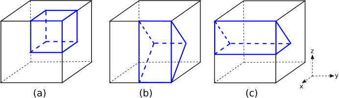
Figure 3: Illustration of irreducible subdomain $\Omega_{0}$. (a) For $D_{2h}$ it is a small cube; (b) For $D_{4}$, a triangular prism; (c) For $D_{2d}$ also a triangular prism, with a different shape.

We employ trilinear finite elements to solve these eigenvalue subproblems, and see from the convergence rate of eigenvalues that the implementation is correct. Taking non-Abelian group $D_{4}$ for instance, we exhibit errors in eigenvalue approximations obtained from solving the subproblems in Figure 4. And the $h^{2}$-convergence rate can be observed.

Moreover, in Table 4, we list the $\nu$-$l$ symmetries of computed eigenfunctions from solving the subproblems. We observe that the required 10 eigenpairs are distributed over subproblems, i.e., each subproblem only needs to solve a smaller number of eigenpairs.

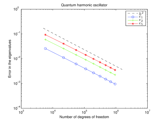
Figure 4: Errors in the eigenvalue approximations from solving 6 subproblems associated with non-Abelian group $D_{4}$ using trilinear finite elements. Errors in the first three different eigenvalues 1.5, 2.5 and 3.5 are labeled as $e_{1}$, $e_{2}$ and $e_{5}$, respectively. The $h^{2}$-convergence rate can be observed.

Table 4: The $\nu$-$l$ symmetries of the first 10 computed eigenfunctions from solving subproblems. The $\nu$-$l$ values indicate which subproblem each eigenfunction belongs to, where $\nu\in\{1,2,\ldots,n_{c}\}$ and $l\in\{1,2,\ldots,d_{\nu}\}$. In the case of $D_{2h}$, all the $l$ values are 1 because it is an Abelian group and all irreducible representations are one-dimensional, i.e., $d_{\nu}=1$ for all $\nu=1,2,\ldots,8$.

		$u_{1}$	$u_{2}$	$u_{3}$	$u_{4}$	$u_{5}$	$u_{6}$	$u_{7}$	$u_{8}$	$u_{9}$	$u_{10}$
$D_{2h}$	$\nu$	1	8	6	7	3	4	2	1	1	1
	$l$	1	1	1	1	1	1	1	1	1	1
$D_{4}$	$\nu$	1	3	5	5	5	5	4	1	2	1
	$l$	1	1	1	2	1	2	1	1	1	1
$D_{2d}$	$\nu$	1	5	5	2	4	5	5	1	2	1
	$l$	1	1	2	1	1	1	2	1	1	1

6.2 Reduction in computational cost

Taking Abelian group $D_{2h}$ as an example, we compare the computational cost of solving the original eigenvalue problem (6.1) with that of solving 8 subproblems. We compute the first 110 eigenvalues of the original eigenvalue problem. And it is sufficient to solve the first 22 eigenvalues of each subproblem. In order to illustrate and analyze the saving in computational cost, we launch the tests on a single CPU core.

In Table 5, we present statistics from trilinear finite element discretizations. We see that the average CPU time of a single iteration during solving the original problem (6.1) is 42.29 seconds while that of solving 8 subproblems is 3.61 seconds . In Table 6, we present statistics from tricubic finite element discretizations. We observe that the average CPU time of a single iteration during solving the original problem (6.1) is 60.80 seconds while that of solving 8 subproblems is 9.71 seconds.

Table 5: Statistics of solving the original problem (6.1) and 8 subproblems using trilinear finite elements. In Column 1, subproblems are labeled by different $\nu$ values. In Columns 2 and 3, we list the number of iteration steps and matrix-vector multiplications. In Columns 4 and 5, we present CPU time spent on matrix-vector multiplications and the whole procedure of IRLM.

Problem	#Iter.	#OP*x	time_mv (sec.)	time_total (sec.)
(6.1)	22	1599	175.01	930.39
$\nu=1$	18	356	5.13	8.21
$\nu=2$	22	420	6.16	9.95
$\nu=3$	22	421	6.06	9.83
$\nu=4$	21	406	5.84	9.46
$\nu=5$	18	353	5.06	8.23
$\nu=6$	21	405	5.74	9.44
$\nu=7$	20	389	5.51	9.03
$\nu=8$	21	403	5.75	9.34

Table 6: Statistics of solving (6.1) and 8 subproblems using tricubic finite elements.

Problem	#Iter.	#OP*x	time_mv (sec.)	time_total (sec.)
(6.1)	57	3972	1696.29	3465.57
$\nu=1$	50	937	55.15	62.75
$\nu=2$	64	1156	67.75	77.11
$\nu=3$	64	1153	67.57	77.09
$\nu=4$	62	1128	66.05	75.25
$\nu=5$	47	892	52.18	59.31
$\nu=6$	69	1215	71.15	81.37
$\nu=7$	63	1134	66.74	76.12
$\nu=8$	70	1230	72.46	82.87

We note that the speedup in average CPU time of a single iteration is 11.71 with trilinear finite elements while it is decreased to 6.26 with tricubic finite elements. This numerical phenomenon can be explained by performance analysis (4.4). In our computation, the maximum dimension of Krylov subspace is twice the number of required eigenpairs plus 5, which is recommended by ARPACK’s tutorial examples. So we have $\theta_{1}=4.59$. We obtain from the statistics of solving the original problem that the CPU time percentage $\omega$ of matrix-vector multiplications is 0.19 with trilinear finite elements and grows to 0.49 with tricubic finite elements. Correspondingly, using (4.4), we predict that the CPU time speedup for trilinear and tricubic finite elements would be 12.52 and 7.64, respectively.

We see from (4.2) that the computational cost of $QR$-iteration grows faster than that of matrix-vector multiplication when the number of required eigenpairs increases. Thus we can expect that the decomposition approach would be more appreciable for large-scale eigenvalue problems.

6.3 Saving in communication

Besides the reduction in computational cost, solving decoupled problems will also save communication among parallel processors. As mentioned in Section 5.3, our implementation of the decomposition approach is parallelized in two levels. No communication occurs between any two groups of processors during solving the eigenvalue problem. This leads to a saving in communication.

For illustration, we take the oscillator eigenvalue problem (6.1) as an example. We decompose it into 8 decoupled subproblems according to group $D_{2h}$. The comparison of communication between solving the original problem and the subproblems is given in Table 7.

Table 7: Comparison of communication between solving (6.1) and 8 subproblems. Column 1 gives the number of processors. In the other columns, “use symm” represents solving subproblems and “not use” means solving the original eigenvalue problem. Columns 2 and 3 give the average number of processors each processor communicates with. Columns 4 and 5 list the average number of Bytes sent by each processor. And the last two columns report the CPU time spent on communication during matrix-vector multiplications.

$N_{p}$	$N_{p}$ in comm		Bytes in comm		CPU time in comm (sec.)
	use symm	not use	use symm	not use	use symm	not use
8	0.00	1.75	0	134,560	0.00	8.93
16	1.00	1.88	19,608	145,451	0.20	10.36

6.4 Applications to Kohn–Sham equations

Now we apply the decomposition approach to electronic structure calculations of symmetric molecules, based on code RealSPACES (Real Space Parallel Adaptive Calculation of Electronic Structure) of the LSEC of Chinese Academy of Sciences. In the context of density functional theory (DFT), ground state properties of molecular systems are usually obtained by solving the Kohn–Sham equation [30, 34, 38]. It is a nonlinear eigenvalue problem as follows

$$\left(-\frac{1}{2}\Delta+V^{\mbox{eff}}[\rho]\right)\Psi_{n}=\epsilon_{n}\Psi_{n}\quad\mbox{in}~{}\mathbb{R}^{3},$$ (6.4)

where $\rho({\bf r})=\sum_{n=1}^{N_{e}}f_{n}\left|\Psi_{n}({\bf r})\right|^{2}$ is the charge density contributed by $N_{e}$ eigenfunctions $\{\Psi_{n}\}$ with occupancy numbers $\{f_{n}\}$, and $V^{\mbox{eff}}[\rho]$ the so-called effective potential which is a nonlinear functional of $\rho$. On the assumption of no external fields, $V^{\mbox{eff}}[\rho]$ can be written into

$$V^{\mbox{eff}}=V^{\mbox{ne}}+V^{\mbox{\small H}}+V^{\mbox{xc}},$$

where $V^{\mbox{ne}}$ is the Coulomb potential between the nuclei and the electrons, $V^{\mbox{\small H}}$ the Hartree potential, and $V^{\mbox{xc}}$ the exchange-correlation potential [38]. The ground state density of a confined system decays exponentially [2, 22, 44], so we choose the computational domain as an appropriate cube and impose zero boundary condition.

As a nonlinear eigenvalue problem, Kohn–Sham equation (6.4) is solved by the self-consistent field (SCF) iteration [38]. The dominant part of computation is the repeated solving of the linearized Kohn–Sham equation with a fixed effective potential. The number of required eigenstates grows in proportion to the number of valence electrons in the system. Therefore the Kohn–Sham equation solver will probably make the performance bottleneck for large-scale DFT calculations.

Real-space discretization methods are attractive for confined systems since they allow a natural imposition of the zero boundary condition [6, 17, 35]. Among real-space mesh techniques, the finite element method keeps both locality and the variational property, and has been successfully applied to electronic structure calculations (see, e.g., [1, 19, 20, 26, 42, 43, 45, 46, 50, 51, 54]); others like the finite difference method, finite volume method and the wavelet approach have also shown the potential in this field [13, 17, 23, 28, 32, 35, 41].

We solve the Kohn–Sham equation of some symmetric molecules with tricubic finite element discretizations. The statistics are summarized in Table 9. The full symmetry group of these molecules is the tetrahedral group $T_{d}$. For simplicity we select subgroup $D_{2}$ as shown in Table 8 [14]. Accordingly, the Kohn–Sham equation can be decomposed into 4 decoupled subproblems. It is indicated by the increasing speedup in Table 9 that the decomposition approach is appreciable for large-scale symmetric molecular systems.

Table 8: Representation matrices of Abelian group $D_{2}$. It has 4 symmetry operations, i.e., order $g=4$, and thus has $n_{c}=4$ one-dimensional irreducible representations. We refer to Appendix A for a description of symmetry operations.

$D_{2}$	$E$	$C_{2x}$	$C_{2y}$	$C_{2z}$
$\Gamma^{(1)}$	1	1	1	1
$\Gamma^{(2)}$	1	1	-1	-1
$\Gamma^{(3)}$	1	-1	1	-1
$\Gamma^{(4)}$	1	-1	-1	1

Table 9: Comparison between solving the original Kohn–Sham equation and subproblems. Column 3 gives the number of required eigenstates. The number of degrees of freedom given in Columns 4 and 5 is required by the convergence of ground state energy [19]. Columns 7 and 8 list the average CPU time in diagonalization at each SCF iteration step, which is the dominant part of time. The last column is the speedup of the decomposition approach.

System	$G$	$N_{e}$	$N$	$N_{0}$	$N_{p}$	CPU time in diag. (sec.)		Speedup
						not use	use symm
$\mbox{C}_{123}\mbox{H}_{100}$	$D_{2}$	300	1,191,016	297,754	32	2,783	558	4.99
$\mbox{C}_{275}\mbox{H}_{172}$	$D_{2}$	640	1,643,032	410,758	32	13,851	1,559	8.88
$\mbox{C}_{525}\mbox{H}_{276}$	$D_{2}$	1200	2,097,152	524,288	64	25,296	2,334	10.84

7 Concluding remarks

In this paper, we have proposed a decomposition approach to eigenvalue problems with spatial symmetries. We have formulated a set of eigenvalue subproblems friendly for grid-based discretizations. Different from the classical treatment of symmetries in quantum chemistry, our approach does not explicitly construct symmetry-adapted bases. However, we have provided a construction procedure for the symmetry-adapted bases, from which we have obtained the relation between the two approaches.

Note that such a decomposition approach can reduce the computational cost remarkably since only a smaller number of eigenpairs are solved for each subproblem and the subproblems can be solved in a smaller subdomain. We would believe that the quantization of this reduction implies that our approach could be appreciable for large-scale eigenvalue problems. In practice, we solve a sufficient number of redundant eigenpairs for each subproblem in order not to miss any eigenpairs. It would be very helpful for reducing the extra work if one could predict the distribution of eigenpairs among subproblems.

Under finite element discretizations, our decomposition approach has been applied to Kohn–Sham equations of symmetric molecules. If solving Kohn–Sham equations of periodic crystals, we should consider plane wave expansion which could be regarded as grid-based discretization in reciprocal space. In Appendix C, we show that the invariance under some coordinate transformation can be kept by Fourier transformation. So the decomposition approach would be applicable to plane waves, too.

Currently, we have imposed an odd number of partition and used finite elements of odd orders to avoid degrees of freedom on symmetry elements. In numerical examples, we have treated only a part of cubic symmetries for validation and illustration. Obviously, the decomposition approach and its practical issues can be adapted to other spatial symmetries with appropriate grids.

In this paper, we concentrate on spatial symmetries only. It is possible to use other symmetries to reduce the computational cost, too. For instance, the angular momentum, spin and parity symmetries of atoms have been exploited during solving the Schrödinger equation in [21, 39]; the total particle number and the total spin $z$-component, except for rotational and translational symmetries, have been taken into account to block-diagonalize the local (impurity) Hamiltonian in the computation of dynamical mean-field theory for strongly correlated systems [25, 29]. It is our future work to exploit these underlying or internal symmetries.

Appendix A: Basic concept of group theory

In this appendix, we include some basic concepts of group theory for a more self-contained exposition. They could be found in standard textbooks like [8, 14, 15, 33, 47, 52].

A group $G$ is a set of elements $\{R\}$ with a well-defined multiplication operation which satisfy several requirements:

1. The set is closed under the multiplication.

2. The associative law holds.

3. There exists a unit element $E$ such that $ER=RE=R$ for any $R\in G$.

4. There is an inverse $R^{-1}$ in $G$ to each element $R$ such that $RR^{-1}=R^{-1}R=E$.

If the commutative law of multiplication also holds, $G$ is called an Abelian group. Group $G$ is called a finite group if it contains a finite number of elements. And this number, denoted by $g$, is said to be the order of the group. The rearrangement theorem tells that the elements of $G$ are only rearranged by multiplying each by any $R\in G$, i.e., $RG=G$ for any $R\in G$.

An element $R_{1}\in G$ is called to be conjugate to $R_{2}$ if $R_{2}=SR_{1}S^{-1}$, where $S$ is some element in the group. All the mutually conjugate elements form a class of elements. It can be proved that group $G$ can be divided into distinct classes. Denote the number of classes as $n_{c}$. In an Abelian group, any two elements are commutative, so each element forms a class by itself, and $n_{c}$ equals the order of the group.

Two groups is called to be homomorphic if there exists a correspondence between the elements of the two groups as $R\leftrightarrow R^{\prime}_{1},R^{\prime}_{2},\ldots$, which means that if $RS=T$ then the product of any $R^{\prime}_{i}$ with any $S^{\prime}_{j}$ will be a member of the set $\{T^{\prime}_{1},T^{\prime}_{2},\ldots\}$. In general, a homomorphism is a many-to-one correspondence. It specializes to an isomorphism if the correspondence is one-to-one.

A representation of a group is any group of mathematical entities which is homomorphic to the original group. We restrict the discussion to matrix representations. Any matrices representation with nonvanishing determinants is equivalent to a representation by unitary matrices. Two representations are said to be equivalent if they are associated by a similarity transformation. If a representation can not be equivalent to representations of lower dimensionality, it is called irreducible.

The number of all the inequivalent, irreducible, unitary representations is equal to $n_{c}$, which is the number of classes in $G$. The Celebrated Theorem tells that

$$\sum_{\nu=1}^{n_{c}}d_{\nu}^{2}=g,$$

where $d_{\nu}$ denotes the dimensionality of the $\nu$-th representation. Since the number of classes of an Abelian group equals the number of elements, an Abelian group of order $g$ has $g$ one-dimensional irreducible representations.

The groups used in this paper are all crystallographic point groups. Groups $D_{2}$, $D_{2h}$, $D_{2d}$ and $D_{4}$ are four dihedral groups; the first two groups are Abelian and the other two are non-Abelian. In Table 3 and Table 8, $C_{nj}$ denotes a rotation about axis $Oj$ by $2\pi/n$ in the right-hand screw sense and $I$ is the inversion operation [14]. The $Oj$ axes are illustrated in Figure 5. We refer to textbooks like [8, 14, 15, 47] for more details about crystallographic point groups.

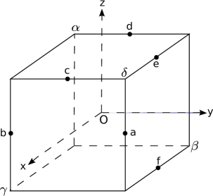
Figure 5: Rotation axes in Table 3 and Table 8

Appendix B: Proof of Proposition 2.2

Proof.

(a) Since $\{P_{R}\}$ are unitary operators, we have

$${\mathscr{P}^{(\nu)}_{ml}}^{*}=\left(\frac{d_{\nu}}{g}\sum_{R\in G}{\Gamma^{(\nu)}(R)}^{*}_{ml}P_{R}\right)^{*}=\frac{d_{\nu}}{g}\sum_{R\in G}\Gamma^{(\nu)}(R)_{ml}P_{R^{-1}}=\frac{d_{\nu}}{g}\sum_{S\in G}\Gamma^{(\nu)}(S^{-1})_{ml}P_{S},$$

which together with the fact that $\Gamma^{(\nu)}$ is a unitary representation derives

$${\mathscr{P}^{(\nu)}_{ml}}^{*}=\frac{d_{\nu}}{g}\sum_{S\in G}{\Gamma^{(\nu)}(S)}^{*}_{lm}P_{S}=\mathscr{P}^{(\nu)}_{lm}.$$

(b) It follows from the definition that

$$\mathscr{P}^{(\nu)}_{ml}\mathscr{P}^{(\nu^{\prime})}_{m^{\prime}l^{\prime}} = \left(\frac{d_{\nu}}{g}\sum_{R\in G}{\Gamma^{(\nu)}(R)}^{*}_{ml}P_{R}\right)\left(\frac{d_{\nu^{\prime}}}{g}\sum_{S\in G}{\Gamma^{(\nu^{\prime})}(S)}^{*}_{m^{\prime}l^{\prime}}P_{S}\right)$$

$$= \frac{d_{\nu}d_{\nu^{\prime}}}{g^{2}}\sum_{R\in G}{\Gamma^{(\nu)}(R)}^{*}_{ml}\left(\sum_{S\in G}{\Gamma^{(\nu^{\prime})}(S)}^{*}_{m^{\prime}l^{\prime}}P_{RS}\right).$$

Note that the rearrangement theorem implies that, when $S$ runs over all the group elements, $S^{\prime}=RS$ for any $R$ also runs over all the elements. Hence we get

$$\mathscr{P}^{(\nu)}_{ml}\mathscr{P}^{(\nu^{\prime})}_{m^{\prime}l^{\prime}} = \frac{d_{\nu}d_{\nu^{\prime}}}{g^{2}}\sum_{R\in G}{\Gamma^{(\nu)}(R)}^{*}_{ml}\left(\sum_{S^{\prime}\in G}{\Gamma^{(\nu^{\prime})}(R^{-1}S^{\prime})}^{*}_{m^{\prime}l^{\prime}}P_{S^{\prime}}\right)$$

$$= \frac{d_{\nu}d_{\nu^{\prime}}}{g^{2}}\sum_{S^{\prime}\in G}\left(\sum_{R\in G}{\Gamma^{(\nu)}(R)}^{*}_{ml}~{}{\Gamma^{(\nu^{\prime})}(R^{-1}S^{\prime})}^{*}_{m^{\prime}l^{\prime}}\right)P_{S^{\prime}}.$$

We may calculate as follows

$$\sum_{R\in G}{\Gamma^{(\nu)}(R)}^{*}_{ml}{\Gamma^{(\nu^{\prime})}(R^{-1}S^{\prime})}^{*}_{m^{\prime}l^{\prime}} = \sum_{R\in G}{\Gamma^{(\nu)}(R)}^{*}_{ml}\left(\sum_{n=1}^{d_{\nu^{\prime}}}{\Gamma^{(\nu^{\prime})}(R^{-1})}^{*}_{m^{\prime}n}~{}{\Gamma^{(\nu^{\prime})}(S^{\prime})}^{*}_{nl^{\prime}}\right)$$

$$= \sum_{R\in G}{\Gamma^{(\nu)}(R)}^{*}_{ml}\left(\sum_{n=1}^{d_{\nu^{\prime}}}{\Gamma^{(\nu^{\prime})}(R)}_{nm^{\prime}}~{}{\Gamma^{(\nu^{\prime})}(S^{\prime})}^{*}_{nl^{\prime}}\right)$$

$$= \sum_{n=1}^{d_{\nu^{\prime}}}{\Gamma^{(\nu^{\prime})}(S^{\prime})}^{*}_{nl^{\prime}}\left(\sum_{R\in G}{\Gamma^{(\nu)}(R)}^{*}_{ml}~{}{\Gamma^{(\nu^{\prime})}(R)}_{nm^{\prime}}\right),$$

which together with the great orthogonality theorem yields

$$\sum_{R\in G}{\Gamma^{(\nu)}(R)}^{*}_{ml}{\Gamma^{(\nu^{\prime})}(R^{-1}S^{\prime})}^{*}_{m^{\prime}l^{\prime}}=\delta_{\nu\nu^{\prime}}\delta_{lm^{\prime}}\frac{g}{d_{\nu^{\prime}}}{\Gamma^{(\nu)}(S^{\prime})}^{*}_{ml^{\prime}}.$$

Thus we arrive at

$$\mathscr{P}^{(\nu)}_{ml}\mathscr{P}^{(\nu^{\prime})}_{m^{\prime}l^{\prime}}=\delta_{\nu\nu^{\prime}}\delta_{lm^{\prime}}\frac{d_{\nu}}{g}\sum_{S^{\prime}\in G}{\Gamma^{(\nu)}(S^{\prime})}^{*}_{ml^{\prime}}P_{S^{\prime}}=\delta_{\nu\nu^{\prime}}\delta_{lm^{\prime}}\mathscr{P}^{(\nu)}_{ml^{\prime}}.$$

∎

Appendix C: Spatial symmetry in reciprocal space

Plane wave method is widely used for solving the Kohn–Sham equations of crystals. Actually, plane waves may be regarded as grid-based discretizations in reciprocal space. We will show that the symmetry relation in real space is kept in reciprocal space. The solution domain $\Omega$ of crystals can be spanned by three lattice vectors in real space. We denote them as ${\bf a}_{i}(i=1,2,3)$. If function $f$ is invariant with integer multiple translations of the lattice vectors, we then present the function in reciprocal space as like:

$$\hat{f}({\bf q})=\frac{1}{N}\sum_{\bf{r}}f({\bf r})e^{-\imath{\bf q}\cdot{\bf r}},$$

where ${\bf q}$ is any vector in reciprocal space satisfying ${\bf q}\cdot{\bf a}_{i}=2\pi\frac{n}{N_{i}}$ with $n$ an integer, $N_{i}$ the number of degrees of freedom along direction ${\bf a}_{i}~{}(i=1,2,3)$, and $N=N_{1}N_{2}N_{3}$ the total number of degrees of freedom. Assume that $f$ is kept invariant under coordinate transformation $R$ in $\Omega$. We obtain from

$$\hat{f}(R{\bf q})=\frac{1}{N}\sum_{{\bf r}}f({\bf r})e^{-\imath(R{\bf q})\cdot{\bf r}}$$

and the coordinate transformation $R$ can be represented as an orthogonal matrix that

$$\hat{f}(R{\bf q})=\frac{1}{N}\sum_{{\bf r}}f({\bf r})e^{-\imath{\bf q}\cdot\left(R^{-1}{\bf r}\right)}.$$

Since

$$f(R^{-1}{\bf r})=f({\bf r})\quad\forall{\bf r}\in\Omega,$$

we have

$$\hat{f}(R{\bf q})=\frac{1}{N}\sum_{R^{-1}{\bf r}}f(R^{-1}{\bf r})e^{-\imath{\bf q}\cdot\left(R^{-1}{\bf r}\right)}=\hat{f}({\bf q}).$$

Hence the decomposition approach is probably applicable to plane waves.

Acknowledgements. The authors would like to thank Prof. Xiaoying Dai, Prof. Xingao Gong, Prof. Lihua Shen, Dr. Zhang Yang, and Mr. Jinwei Zhu for their stimulating discussions on electronic structure calculations. The second author is grateful to Prof. Zeyao Mo for his encouragement.

References

- [1] J. Ackermann, B. Erdmann, and R. Roitzsch. A self-adaptive multilevel finite element method for the stationary Schrödinger equation in three space dimensions. J. Chem. Phys., 101:7643–7650, 1994.
- [2] S. Agmon. Lectures on the Exponential Decay of Solutions of Second-Order Elliptic Operators. Princeton University Press, Princeton, NJ, 1981.
- [3] I. Babuska and J. E. Osborn. Finite element-Galerkin approximation of the eigenvalues and eigenvectors of self-adjoint problems. Math. Comput., 52(186):275–297, 1989.
- [4] I. Babuska and J. Osborn. Eigenvalue problems. In Handbook of Numerical Analysis, volume II, pages 641–787. North-Holland, 1991.
- [5] L. Banjai. Eigenfrequencies of fractal drums. J. Comput. Appl. Math., 198:1–18, 2007.
- [6] T. L. Beck. Real-space mesh techniques in density-functional theory. Rev. Mod. Phys., 72:1041–1080, 2000.
- [7] J. K. Bennighof and R. B. Lehoucq. An automated multilevel substructuring method for eigenspace computation in linear elastodynamics. SIAM J. Sci. Comput., 25:2084–2106, 2004.
- [8] D. M. Bishop. Group Theory and Chemistry. Dover, New York, 1993.
- [9] A. Bossavit. Symmetry, groups, and boundary value problems. A progressive introduction to noncommutative harmonic analysis of partial differential equations in domains with geometrical symmetry. Comp. Meth. Appl. Mech. Engng., 56:167–215, 1986.
- [10] A. Bossavit. Boundary value problems with symmetry, and their approximation by finite elements. SIAM J. Appl. Math., 53:1352–80, 1993.
- [11] E. Cances, M. Defranceschi, W. Kutzelnigg, C. Le Bris, and Y. Mada. Computational quantum chemistry: a primer. In Ph. G. Ciarlet and C. Le Bris, editors, Handbook of Numerical Analysis, Special volume, Computational Chemistry, Volume X, pages 3–270. North-Holland, 2003.
- [12] F. Chatelin, Spectral Approximations of Linear Operators, Academic Press, New York, 1983.
- [13] J. R. Chelikowsky, N. Troullier, and Y. Saad. Finite-difference-pseudopotential method: Electronic structure calculations without a basis. Phys. Rev. Lett., 72:1240–1243, 1994.
- [14] J. F. Cornwell. Group Theory in Physics: An Introduction. Academic Press, California, 1997.
- [15] F. A. Cotton. Chemical Applications of Group Theory. John Wiley and Sons, New York, 3rd edition, 1990.
- [16] R. R. Craig, Jr. and M. C. C. Bampton. Coupling of substructures for dynamic analysis. AIAA J., 6:1313–1319, 1968.
- [17] X. Dai, X. Gong, Z. Yang, D. Zhang, and A. Zhou. Finite volume discretizations for eigenvalue problems with applications to electronic structure calculations. Multiscale Model. Simul., 9:208–240, 2011.
- [18] X. Dai, Z. Yang, and A. Zhou, Symmetric finite volume schemes for eigenvalue problems in arbitrary dimensions, Sci. China Ser. A, 51:1401–1414, 2008.
- [19] J. Fang, X. Gao, and A. Zhou. A Kohn–Sham equation solver based on hexahedral finite elements. J. Comput. Phys., 231:3166–3180, 2012.
- [20] J.-L. Fattebert, R. D. Hornung, and A. M. Wissink. Finite element approach for density functional theory calculations on locally-refined meshes. J. Comput. Phys., 223:759–773, 2007.
- [21] G. Friesecke and B. D. Goddard. Asymptotics-based CI models for atoms: properties, exact solution of a minimal model for Li to Ne, and application to atomic spectra. Multiscale Model. Simul., 7:1876–1897, 2009.
- [22] L. Gårding, On the essential spectrum of Schrödinger operators, J. Funct. Anal., 52:1–10, 1983.
- [23] L. Genovese, A. Neelov, S. Goedecker, T. Deutsch, S. A. Ghasemi, A. Willand, D. Caliste, O. Zilberberg, M. Rayson, A. Bergman, and R. Schneider. Daubechies wavelets as a basis set for density functional pseudopotential calculations. J. Chem. Phys., 129:014109, 2008.
- [24] G. H. Golub and C. F. van Loan. Matrix Compuations. Johns Hopkins University Press, 1996.
- [25] E. Gull, A. J. Millis, A. I. Lichtenstein, A. N. Rubtsov, M. Troyer, and P. Werner Continuous-time Monte Carlo methods for quantum impurity models. Rev. Mod. Phys., 83:349–404, 2011.
- [26] X. Gong, L. Shen, D. Zhang, and A. Zhou. Finite element approximations for Schrödinger equations with applications to electronic structure computations. J. Comput. Math., 23:310-327, 2008.
- [27] W. Hackbusch. Elliptic Differential Equations: Theory and Numerical Treatment. Springer-Verlag, Berlin Heidelberg, 1992.
- [28] Y. Hasegawa, J.-I. Iwata, M. Tsuji, D. Takahashi, A. Oshiyama, K. Minami, T. Boku, F. Shoji, A. Uno, M. Kurokawa, H. Inoue, I. Miyoshi, and M. Yokokawa. First-principles calculations of electron states of a silicon nanowire with 100,000 atoms on the K computer. In Proceedings of 2011 International Conference for High Performance Computing, Networking, Storage and Analysis (SC2011), pages 1–11, 2011.
- [29] K. Haule. Quantum Monte Carlo impurity solver for cluster dynamical mean-field theory and electronic structure calculations with adjustable cluster base. Phys. Rev. B, 75:155113, 2007.
- [30] P. Hohenberg and W. Kohn. Inhomogeneous electron gas. Phys. Rev. B, 136(3B):B864–B871, 1964.
- [31] W. C. Hurty. Vibrations of structure systems by component-mode synthesis. ASCE J. Engng. Mech. Division, 86:51–69, 1960.
- [32] J.-I. Iwata, D. Takahashi, A. Oshiyama, T. Boku, K. Shiraishi, S. Okada, and K. Yabana. A massively-parallel electronic-structure calculations based on real-space density functional theory. J. Comput. Phys., 229:2339–2363, 2010.
- [33] H. Jones. The Theory of Brillouin Zones and Electronic States in Crystals. North-Holland, Amsterdam, 1960.
- [34] W. Kohn and L. J. Sham. Self-consistent equations including exchange and correlation effects. Phys. Rev., 140(4A):A1133–A1138, 1965.
- [35] L. Kronik, A. Makmal, M. L. Tiago, M. M. G. Alemany, M. Jain, X. Huang, Y. Saad, and J. R. Chelikowsky. Parsec – the pseudopotential algorithm for real-space electronic structure calculations: recent advances and novel applications to nano-structures. Phys. Stat. Sol. (b), 243:1063–1079, 2006.
- [36] J. R. Kuttler and V. G. Sigillito. Eigenvalues of the Laplacian in two dimensions. SIAM Rev., 26:163–193, 1984.
- [37] R. B. Lehoucq, D. C. Sorensen, and C. Yang. ARPACK Users’ Guide: Solution of Large-scale Eigenvalue Problems with Implicitly Restarted Arnoldi Methods. SIAM, Philadelphia, 1998.
- [38] R. M. Martin. Electronic Structure: Basic Theory and Practical Methods. Cambridge University Press, Cambridge, 2004.
- [39] C. B. Mendl and G. Friesecke. Efficient algorithm for asymptotics-based configuration-interaction methods and electronic structure of transition metal atoms. J. Chem. Phys., 133:184101, 2010.
- [40] J. M. Neuberger, N. Sieben, and J. W. Swift. Computing eigenfunctions on the Koch Snowflake: A new grid and symmetry. J. Comput. Appl. Math., 191:126–142, 2006.
- [41] T. Ono and K. Hirose. Real-space electronic-structure calculations with a time-saving double-grid technique. Phys. Rev. B, 72:085115, 2005.
- [42] J. E. Pask, B. M. Klein, C. Y. Fong, and P. A. Sterne. Real-space local polynomial basis for solid-state electronic-structure calculations: A finite-element approach. Phys. Rev. B, 59:12352–11358, 1999.
- [43] J. E. Pask and P. A. Sterne. Finite element methods in ab initio electronic structure calculations. Model. Simul. Mater. Sci. Eng., 13:71–96, 2005.
- [44] B. Simon. Schrödinger operators in the twentieth century. J. Math. Phys., 41:3523–3555, 2000.
- [45] P. A. Sterne, J. E. Pask, and B. M. Klein. Calculation of positron observables using a finite element-based approach. Appl. Surf. Sci., 149:238–243, 1999.
- [46] P. Suryanarayana, V. Gavini, and T. Blesgen. Non-periodic finite-element formulation of Kohn–Sham density functional theory. J. Mech. Phys. Solids, 58:256–280, 2010.
- [47] M. Tinkham. Group Theory and Quantum Mechanics. McGraw-Hill, New York, 1964.
- [48] T. Torsti, T. Eirola, J. Enkovaara, T. Hakala, P. Havu, V. Havu, T. Höynälänmaa, J. Ignatius, M. Lyly, I. Makkonen, T. T. Rantala, J. Ruokolainen, K. Ruotsalainen, E. Räsänen, H. Saarikoski, and M. J. Puska, Three real-space discretization techniques in electronic structure calculations, Phys. Stat. Sol., B243:1016-1053, 2006.
- [49] L. N. Trefethen and T. Betcke. Computed eigenmodes of planar regions. In Recent advances in differential equations and mathematical physics, volume 412 of Contemp. Math., pages 297–314, Providence, RI, 2006. Amer. Math. Soc.
- [50] E. Tsuchida and M. Tsukada. Electronic-structure calculations based on the finite-element method. Phys. Rev. B, 52:5573–5578, 1995.
- [51] S. R. White, J. W. Wilkins, and M. P. Teter. Finite-element method for electronic structure. Phys. Rev. B, 39:5819–5833, 1989.
- [52] E. P. Wigner. Group Theory and its Application to the Quantum Mechanics of Atomic Spectra. Academic Press, New York, 1959.
- [53] D. C. Young. Computational Chemistry: A Practical Guide for Applying Techniques to Real-World Problems. John Wiley and Sons, New York, 2001.
- [54] D. Zhang, L. Shen, A. Zhou, and X. Gong. Finite element method for solving Kohn–Sham equations based on self-adaptive tetrahedral mesh. Phys. Lett. A, 372:5071–5076, 2008.
- [55] O. C. Zienkiewicz and R. L. Taylor. The Finite Element Method for Solid and Structural Mechanics. Elsevier, London, 6th edition, 2005.