Anderson Localization in Metamaterials and Other Complex Media

Abstract

We review some recent (mostly ours) results on the Anderson localization of light and electron waves in complex disordered systems, including: (i) left-handed metamaterials, (ii) magneto-active optical structures, (iii) graphene superlattices, and (iv) nonlinear dielectric media. First, we demonstrate that left-handed metamaterials can significantly suppress localization of light and lead to an anomalously enhanced transmission. This suppression is essential at the long-wavelength limit in the case of normal incidence, at specific angles of oblique incidence (Brewster anomaly), and in the vicinity of the zero-$\varepsilon$ or zero-$\mu$ frequencies for dispersive metamaterials. Remarkably, in disordered samples comprised of alternating normal and left-handed metamaterials, the reciprocal Lyapunov exponent and reciprocal transmittance increment can differ from each other. Second, we study magneto-active multilayered structures, which exhibit nonreciprocal localization of light depending on the direction of propagation and on the polarization. At resonant frequencies or realizations, such nonreciprocity results in effectively unidirectional transport of light. Third, we discuss the analogy between the wave propagation through multilayered samples with metamaterials and the charge transport in graphene, which enables a simple physical explanation of unusual conductive properties of disordered graphene superlatices. We predict disorder-induced resonances of the transmission coefficient at oblique incidence of the Dirac quasiparticles. Finally, we demonstrate that an interplay of nonlinearity and disorder in dielectric media can lead to bistability of individual localized states excited inside the medium at resonant frequencies. This results in nonreciprocity of the wave transmission and unidirectional transport of light.

I Introduction

Anderson localization is one of the most fundamental phenomena in the physics of disordered systems. Being predicted in the seminal paper And for spin excitations, and then extended to electrons and other one-particle excitations in solids LGP ; Imry and classical waves John ; Ping91 ; Ping07 ; Sok , it became a paradigm of the modern physics AL . The study of this phenomenon remains a hot topic throughout its more than 50-years history. It is constantly stimulated by new experimental results, including the most recent observations in microwaves Genack1 ; we-PRL-1 ; Ref-exp-2 , optics optics ; Segev ; Silberberg , and Bose-Einstein condensates BEC .

Being a universal wave phenomenon, Anderson localization has natural implications in novel exotic wave systems, such as photonic crystals, meta- and magnetooptical materials, graphene superlattices. Indeed, left-handed metamaterials, nonlinear and magnetooptical materials, and graphene  Veselago ; Pendry ; Shalaev ; Katsnelson2 ; Geim ; periodic-1 ; Zvezdin are involved in design and engineering of various multilayered structures operating in a broad spectral range, from optical to microwave frequencies. Random wave scattering and localization naturally appear in such systems, either due to technological imperfections or owing to the intentially designed random lattices. Importantly, exotic properties of the constituent materials essentially require consideration of the interplay of the Anderson localization with various additional effects: absorption and gain FrePusYur ; we-PRL-1 ; gain ; Paasschens ; Asatryan98 , polarization and spin Sipe ; BF ; anti1 ; anti2 , nonlinearity nonlin-loc1 ; nonlin-loc2 ; Silberberg ; Segev ; Shadrivov , and magnetooptical phenomena ErbacherLenkeMaret ; InoueFujii ; Bliokh-mag . In this review, we describe novel remarkable features of Anderson localization of waves in multilayered structures composed of non-conventional materials with unique intrinsic properties.

We start our review with Sec. II which introduces the basic concepts and general formalism describing the wave propagation, scattering, and localization in in random-layered media. Anderson localization originates from the interference of multiply scattered waves, manifesting itself most profoundly in one-dimensional (1D) systems where all states become localized Mott ; Furst . Due to one-dimensional geometry, such systems are well analyzed LGP ; FG ; IKM , including the mathematical level of rigorousness of the results PF ; GMP . We describe the exact transfer-matrix approach to the wave propagation and scattering in layered media. The main spatial scale of localization, i.e., localization length, can be defined in two ways: (i) via the Lyapunov exponent of the random system and (ii) via the decrement of the wave transmission dependent on the system. In usual Anderson-localization problems, these two localization lengths coincide with each other.

In Section III we consider transmission and localization properties of the multilayered H-stacks comprised of normal materials with right-handed $R-$layers and mixed M-stacks, including also left-handed $L-$layers with negative refractive index Veselago . The opposite signs of the phase and group velocities in metamaterials lead to partial or complete cancellation of the phase accumulation in multilayered M-stacks. We show that this cancellation suppresses the interference of multiple scattering waves and the localization itself Asatryan07 ; Asatryan10a ; Asatryan10b ; Asatryan12 . Using the weak scattering approximation (WSA) Asatryan07 ; Asatryan10a , we give detailed analytical and numerical description of transmission and localization properties of both M- and H-stacks and reveal a number of intriguing results. Namely: (i) in the long wave limit localization lengths defined via the Lyapunov exponent and transmission decrement differ from each other in M-stacks, (ii) there exist two ballistic regimes in the H-stacks, (iii) essential suppression of localization at special angles in the case of oblique incidence (Brewster anomaly) and in the vicinity of special frequencies (zero-$\varepsilon$ or zero-$\mu$ frequencies) is observed. Finally, in Section III.7 we discuss an anomalous enhancement Asatryan07 of wave transmission in minimally disordered alternated M-stacks of metamaterials, where the layer thicknesses are equal and only dielectric permittivities (or only magnetic permeabilities) vary.

Section IV is devoted to the study of novel localization features in novel materials. We start with discussion of localization of light propagating through magneto-active multilayered structures, with either Faraday or Cotton-Muton (Voigt) geometries (Section  IV.1). We show that magnetooptical effects can significantly affect the phase relations, resulting in nonreciprocal localization depending on direction of the wave propagation and polarization of light. At resonant frequencies corresponding to the excitation of localized states inside the sample, a nonreciprocal shift of the the resonance results in effectively unidirectional transmission of lightBliokh-mag . In Section  IV.2, conducting properties of a graphene layer subject to stratified electric field are considered. The close analogy between charge transport in such system and wave transmission through multilayered stack BFSN underpins remarkable conductive properties of disordered grapheneCheianov . We predict disorder-induced resonances of the transmission coefficient at oblique incidence of electron waves. Finally, in Section  IV.3, we examine the interplay between nonlinearity and disorder in resonant transmission through a random-leyered dielectric medium Shadrivov . Owing to effective energy localization and pumping, even weak Kerr nonlinearity can play a crucial role leading to bistability of Anderson localized states inside the medium. Akin to the magneto-optical structures, this brings about unidirectional transmission of light.

II Random Multilayered Structures

II.1 Transmission Length and Lyapunov Exponent

As it was mentioned above, 1D Anderson localization results is exponential decay of the transmission coefficient with the length $L$ of the sample. For multilayered systems, it worth to use the total number of layers $N$ and mean layer thickness $L/N$. In what follows we use dimensionless variables measuring all lengths in mean layer thickness units while the time dependence is chosen in the form $e^{-i\omega t}$. For simplicity throughout all this review we mainly consider the lossless stacks. The detailed results concerning to the case of stacks with losses can be found in original works.

Introduce the dimensionless transmission length $l_{N}$ on a realization

$$\frac{1}{l_{N}}=-\frac{\ln|T_{N}|}{N}=-\frac{\mathrm{Re}\ln T_{N}}{N}$$

and ”averaged” $N$-dependent dimensionless transmission length $l_{T}\equiv l_{T}(N)$ of a multilayered $N-$layered stack

$$\frac{1}{l_{T}}=-\left\langle\frac{\ln|T_{N}|}{N}\right\rangle=-\left\langle\frac{\mathrm{Re}\ln T_{N}}{N}\right\rangle.$$ (II.1)

Here $T_{N}$ is the stack amplitude transmission coefficient related to its transmittivity $\mathcal{T}_{N}$ by equality $\mathcal{T}_{N}=|T_{N}|^{2}.$ Due to self-averaging of $\ln|T_{N}|/N$, both these lengths $l_{T}$ and $l_{N}$ tend to the same limit

$$\lim_{N\rightarrow\infty}l_{T}=\lim_{N\rightarrow\infty}l_{N}=l,$$ (II.2)

as the number $N$ of layers tends to infinity. FollowingBaluni we recall $l$ as localization length. This localization length is related directly to the transmission properties. Its reciprocal value is nothing but decrement of the stack transmission coefficient.

Transmission coefficient entering these equations is naturally expressed in terms of the total $T$-matrix of the stack written in the running wave basis. Consider transmission of the plane wave incident normally from the left to the stack comprised of even number $N$ of layers and embedded into free space. In the simplest case, the wave is described in terms of two component vector of, say, an electric field $e.$ Within a uniform medium with dielectric permittivity $\varepsilon$ and magnetic permeability $\mu,$ the field $e$ has the form

$$e(z)=e^{+}e^{ikz}+e^{-}e^{-ikz},\ \ \ \ k=\frac{\omega}{c}\sqrt{\varepsilon\mu},$$ (II.3)

with $z$-axis directed to the right (here and below all lengths of the problem are dimensionless and measured in the mean layer thickness).

If the components of vector ${\vec{e}}$ are normalized by such a way that the energy flux of the wave (II.3) is $|e^{+}|^{2}-|e^{-}|^{2},$ then the amplitudes

$$\vec{e}_{L,R}=\left(\begin{array}[]{c}e^{+}_{L,R}\\ \\ e^{-}_{L,R}\end{array}\right)$$ (II.4)

of the field from both sides out of the $N-$layer stack are related by its transfer matrix ${\hat{T}}(N)$

$${\vec{e}}|_{L}={\hat{T}}(N){\vec{e}}|_{R},$$ (II.5)

which is expressed via transmission and reflection coefficients of the stack as

$${\hat{T}}(N)=\left\|\begin{array}[]{ccc}\displaystyle{\frac{1}{T_{N}}}&&\displaystyle{\frac{R^{*}_{N}}{T^{*}_{N}}}\\ &&\\ \displaystyle{\frac{R_{N}}{T_{N}}}&&\displaystyle{\frac{1}{T^{*}_{N}}}\end{array}\right\|,$$ (II.9)

where asterisk stands for the complex conjugation.

The methods of calculation of transmission coefficient

$$T(N)=\left(\hat{T}_{11}\right)^{-1}$$ (II.10)

are discussed in the next Subsection.

In what follows, we consider stacks composed of weak scattering layers with reflection coefficients of each layer much smaller than $1.$ In spite of this, for a sufficiently long stack the transmission coefficient is exponentially small $\left|T_{N}\right|\sim\exp{(-\kappa N)}$ with decrement coinciding with reciprocal localization length $\kappa=l^{-1}_{T}$ (localized regime). However a short stack comprising a comparatively small number of layers is almost transparent $|R_{N}|^{2}\ll 1$ (ballistic regime). Here the transmission length takes the form

$$l_{T}\approx b=\frac{\langle|R_{N}|^{2}\rangle}{2N},$$ (II.11)

involving the average reflectance Rytov . This follows directly from Eq. (II.1) by virtue of the current conservation relationship, $|R_{N}|^{2}+|T_{N}|^{2}=1$. The length $b$ in this equation is termed the ballistic length.

Accordingly, in studies of the transport of the classical waves in one-dimensional random systems, the following spatial scales arise in a natural way:

• $l_{T}$ — the transmission length of a finite sample (II.1),

• $l$ — the localization length (II.2) related to transmission properties, and

• $b$ — ballistic length (II.11).

The exponential decrease of transmission coefficient with the stack size is only manifestation of Anderson localization. The phenomenon of localization itself is the localized character of eigenstates in infinite disordered system with sufficiently fast decaying correlations. The quantitative characteristic of such a localization is the Lyapunov exponent which is increment of the exponential growth of the currentless state with a given value at certain point far from this point. The amplitude (II.4) of the currentless state in the inhomogeneous medium in the basis of running waves can be parameterized as

$$\vec{e}=e^{\xi}\left(\begin{array}[]{c}e^{i\theta}\\ \\ e^{-i\theta}\end{array}\right)=R\left(\begin{array}[]{c}e^{i\theta}\\ \\ e^{-i\theta}\end{array}\right),$$ (II.12)

where $R(z)$ and $\theta(z)$ are the modulus and the phase of the considered currentless solution correspondingly.

It is knownLGP ; PF that at given initial values $\xi(0)$ ($R(0)$), and $\theta(0)$, the function $\xi(z)$ at a sufficiently far point is approximately proportional to its distance from the initial point. In discrete terms, with the probability $1$ the positive limit exists

$$\gamma=\lim_{N\to\infty}\frac{\xi(N)}{N}=\lim_{N\to\infty}\frac{1}{N}\ln\frac{R(N)}{R(0)},$$ (II.13)

which is called Lyapunov exponent. Its reciprocal value we also call localization length

$$l_{\xi}=\frac{1}{\gamma},$$ (II.14)

however index $\xi$ reminds that this localization length is defined through Lyapunov exponent.

To compare the two localization lengths $l$ and $l_{\xi}$, we consider first the continuous case were corresponding dynamical variable $\xi(z)$ depends on continuous coordinate $z$. In this case, transmittance of the system with length $L$ is exactly expressed asLGP ; GMP

$$\mathcal{T}_{L}\equiv|T_{L}|^{2}=\frac{4}{e^{2\xi_{c}(L)}+e^{2\xi_{s}(L)}+2},$$ (II.15)

where $\xi_{c}(z)$ and $\xi_{s}(z)$ are two independent solutions satisfying so called cosine and sine initial conditions $\theta_{c}(0)=0$ and $\theta(0)=\pi/2$ and having the same limiting behavior

$$\gamma=\frac{1}{l_{\xi}}=\lim_{z\to\infty}\frac{\xi_{c}(z)}{z}=\lim_{z\to\infty}\frac{\xi_{s}(z)}{z}.$$ (II.16)

Equations (II.15) and (II.16) evidently show that in continuous case $l$ and $l_{\xi}$ exactly coincide.

In the discrete case (multilayered stack), corresponding expression for transmittance reads

$$\mathcal{T}_{N}\equiv|T_{N}|^{2}={4}\left(e^{2\xi_{c}(N)}+e^{2\xi_{s}(N)}+\right.$$

$$\left.2e^{\xi_{c}(N)+\xi_{s}(N)}\sin\left(\theta_{c}(N)-\theta_{s}(N)\right)\right)^{-1}.$$ (II.17)

Here the last term in denominator differs from that in Eq. (II.15). Moreover, it can change its sign and generally speaking can essentially reduce the denominator itself thus enlarging transmittance and as a result enlarging localization length $l_{\xi}$ in compare to $l$. Thus, Eqs. (II.1) and (II.13) enable us to state only that $l\geq l_{\xi}$ in contrast to the continuous case where these two localization lengths always coincide. In spite of that, studying of localization in normal disordered multilayered stacks did not show any difference in the two lengths. We will see below that such a difference really manifests itself in the alternated metamaterial stacks.

In this review we are mainly interested in the transmission length $l_{T}$. This quantity can be found directly by standard transmission experiments. At the same time, it is sensitive to the size of the system and therefore is best suited to the description of the transmission properties in both the localized and ballistic regimes. More precisely, the transmission length coincides either with the localization length $l$ or with the ballistic length $b$, respectively in the cases of comparatively long stacks (localized regime) or comparatively short stacks (ballistic regime). That is,

$$l_{T}\approx\left\{\begin{array}[]{ccc}l&&N\gg l\\ &&\\ b&&N\ll b.\end{array}\right..$$

II.2 Transfer Matrices and Weak Scattering Approximation

In this Subsection we describe some methods used for calculation of transmission length and other transmission or/and localization characteristics in various regimes. All of them are based on various versions of transfer matrix approach.

Consider the M-stack alternatively comprised of even number $N$ of uniform layers labeled by index $j=1,...,N$ from right to left, so that all odd layers $j=2n-1,$ are of type “$\alpha$” and all even layers $j=2n$ are of type “$\beta$”, $n=1,2,...,N/2$ (see Fig. 1). In general case the $j-$th layer is characterized by its dimensionless thickness $d_{j}$, dielectric permittivity $\varepsilon_{j}$ and magnetic permeability $\mu_{j}.$

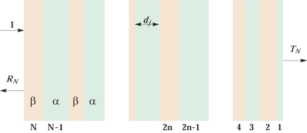
Figure 1: (Ref. [Asatryan07, ]) Two component multilayered alternative stack.

The total transfer matrix (II.9) is factorized to the product

$$\hat{T}(N)={\hat{t}}_{N}{\hat{t}}_{N-1}...{\hat{t}}_{2}{\hat{t}}_{1}$$ (II.18)

of the layer transfer matrices ${\hat{t}}_{j}.$

Note that for considered alternated stack, it is natural to join each pair of subsequent layers with numbers $j=2n-1$ and $j=2n$ into one effective cell number $n$. Then the total transfer matrix factorizes to the product of $N/2$ transfer matrices of separate cells Asatryan07 ; Izra09 ; IMT-10 ; TIM-FNT ; Mak-12 .

Parameterizing the transfer matrix of the $j-$th layer by its transmission $t_{j}$ and reflection $r_{j}$ coefficients of a corresponding layer we obtain the recurrence relations

$$T_{j}=\frac{T_{j-1}t_{j}}{1-R_{j-1}r_{j}},\ \ \ T_{0}=1,$$ (II.19)

$$R_{j}=r_{j}+\frac{R_{j-1}t_{j}^{2}}{1-R_{j-1}r_{j}},\ \ \ R_{0}=0,$$ (II.20)

where $T_{j}$ and $R_{j}$ are transmission and reflection coefficients of the reduced stack comprised of only $j$ first layers. These relations provide an exact description of the system and will be used later for direct numerical simulations of its transmission properties. Another possible but less effective way is related to direct numeric calculation of the total transfer matrix (II.18).

Relations (II.19) and (II.20) serve as a starting point for the weak scattering approximation (WSA) elaborated in Asatryan07 and based on assumption that the reflection from a single layer is small i.e., $\left|r_{j}\right|\ll 1$. This demand is definitely satisfied in the case of weak disorder. Within WSA, instead of exact relations (II.19), (II.20) we use for the transmission length the following first order approximations

$$\ln T_{j} = \ln T_{1,j-1}+\ln t_{j}+R_{j-1}r_{j},$$ (II.21)

$$R_{j} = r_{j}+R_{j-1}t_{j}^{2},\ \ \ j=2,3,...,N.$$ (II.22)

Note that in deriving Eq. (II.22), we omit the first-order term $R_{j-1}^{2}t_{j}^{2}r_{j}.$ This is uncontrolled action. The omitted term contributes only to the second order of $\ln T_{j}$ already after the first iteration for not very large number of layers $j$. For sufficiently large $j,$ it should be taken into account. Nevertheless as we will see below, this approximation is excellent in all wavelength region.

Neglecting the last term in the right hand side of Eq. (II.21) we come to the so-called single-scattering approximation (SSA), which implies that multi-pass reflections are neglected so that the total transmission coefficient is approximated by the product of the single layer transmission coefficients as well as total transmittance is approximated by the product of the single layer transmittances that results in

$$\ln|T_{N}|=\sum_{j=1}^{N}\ln|t_{j}|.$$

In the case of very long stacks (i.e., as the length $N\rightarrow\infty$), we can replace the arithmetic mean, $N^{-1}\sum_{j=1}^{N}\ln|t_{j}|$, by its ensemble average $\langle\ln|t|\rangle.$ On the other hand, in this limit the reciprocal of the transmission length coincides with the localization length. Using the energy conservation law, $|r_{j}|^{2}+|t_{j}|^{2}=1$, which applies in the absence of absorption, the reciprocal localization length in single-scattering approximation may be written as

$$\left(\frac{1}{l}\right)_{ssa}=\frac{1}{2}\langle|r|^{2}\rangle$$

and is proportional to the mean reflectance of a single random layer LGP ; Liansky-1995 .

The version of transfer matrix approach described above is based on consideration of a single layer embedded into vacuum. This version and related WSA were used in Asatryan07 ; Asatryan10a ; Asatryan10b ; Asatryan12 for analytical and numerical study of metamaterial M-stacks (see Section III).

Another version used in Bliokh-mag (Section IV.1) is based on a separation of wave propagation inside a layer and through the interface between layers (see e.g. Ref. BerryKlein ). Here wave propagation inside the $j$-th layer is described by diagonal transfer matrix

$${\hat{S}}_{j}=\mathrm{diag}({\text{e}}^{-i\varphi_{j}},{\text{e}}^{i\varphi_{j}}),$$ (II.23)

where $\varphi_{j}=k_{j}d_{j}$ is the phase accumulated upon the wave propagating from left to right through the $j$-th layer, and $k_{j}=\frac{\omega}{c}\sqrt{\varepsilon_{j}\mu_{j}}.$ The interfaces are described by unimodular transfer matrices ${\hat{F}}^{0\alpha},{\hat{F}}^{\alpha\beta},{\hat{F}}^{\beta\alpha},{\hat{F}}^{\beta 0}$ corresponding, respectively, to transitions (all from left to right) from vacuum to the medium ‘$\alpha$’, from the medium ‘$\alpha$’ to the medium ‘$\beta$’, from the medium ‘$\beta$’ to the medium ‘$\alpha$’, and from the medium ‘$\alpha$’ to vacuum. Thus, the total transfer matrix (II.9) of the structure in Fig. 1 is

$$\hat{T}(N) = {\hat{F}}^{0\alpha}{\hat{F}}_{N}{\hat{S}}_{N}{\hat{F}}_{N-1}{\hat{S}}_{N-1}~{}...~{}{\hat{F}}_{2}{\hat{S}}_{2}{\hat{F}}_{1}{\hat{S}}_{1}{\hat{F}}^{\alpha 0},$$

$$\!\!\!\!\!{\hat{F}}_{2n-1} \equiv {\hat{F}}^{\beta\alpha},~{}{\hat{F}}_{2n}\equiv{\hat{F}}^{\alpha\beta},\ n=1,2,...,N/2.$$ (II.24)

Using the group property of the interface transfer matrices: ${\hat{F}}^{\beta\alpha}={\hat{F}}^{\beta 0}{\hat{F}}^{0\alpha},$ and ${\hat{F}}^{\alpha\beta}={\hat{F}}^{\alpha 0}{\hat{F}}^{0\beta},$ the total transfer matrix is factorized to the product (II.18) where the layer transfer matrices are

$$\hat{t}_{2n}={\hat{F}}^{0\beta}{\hat{S}}_{2n}{\hat{F}}^{\beta 0},\ \ \ \ {\hat{t}}_{2n-1}={\hat{F}}^{0\alpha}{\hat{S}}_{2n-1}{\hat{F}}^{\alpha 0}.$$

Such a representation is especially efficient in the shortwave limit where the total transmission coefficient reduces to the product of the transmission coefficients of only interfaces (see Ref. BerryKlein and Section IV.1).

Come now to application of the transfer matrix approach to calculation of the Lyapunov exponent $\gamma$. Define for each layer the curentless vector $\vec{e}_{j}$ by Eq. (II.12) with the corresponding values $\xi_{j}$ and $\theta_{j}$. In this terms Lyapunov exponent is written as

$$\gamma=\lim_{j\to\infty}\frac{\xi_{j}}{j}=\lim_{j\to\infty}(\xi_{j}-\xi_{j-1}).$$ (II.25)

(we used Shtolz theorem). The vectors $\vec{e}_{j}$ and $\vec{e}_{j-1}$ satisfy the equation

$$\vec{e}_{j}=\hat{t}_{j-1}\vec{e}_{j-1}.$$ (II.26)

Therefore the difference in the r.h.s. of Eq. (II.25) is some function of $\theta_{j-1}$

$$\xi_{j}-\xi_{j-1}=\Phi(\theta_{j-1}),$$ (II.27)

which explicit form is determined by Eq. II.26. Using the self averaging of the ratio $\xi_{j}/j$ and the fact that the phase $\theta_{j}$ stabilizesLGP , we finally obtain for Lyapunov exponent

$$\gamma=\langle\Phi(\theta)\rangle_{\text{st}},$$ (II.28)

where average in the r.h.s. is taken over stationary distribution of the phase $\theta$.

Continuous version of this result was obtained in LGP (see Eq. (10.2)). Its discrete version in slightly different terms (see Section III.7) was obtained in IKT . Note that due to existence of the closed formula (II.28) for Lyapunov exponent, the task of analytical calculation of the localization length $l_{\xi}=\gamma^{-1}$ is a simpler problem than that of transmission length $l_{T}$.

The next steps are standard (see e.g. Refs. [GP, ; LGP, ]): using (II.26) to get the dynamic equation for the phase $\theta$, write down corresponding Fokker-Planck equation for its distribution, solve it and calculate the average (II.28). Moreover, in weakly disordered systems, only the first and the second order terms should be accounted for in the dynamic equations APS ; LGP . For minimally disordered M-stacks defined in Section I, this program was successfully realized in TIM-FNT ; Mak-12 (see Section III.7 below).

III Suppression of Localization in Metamaterials

Over the past decade, the physical properties of metamaterials and their possible applications in modern optics and microelectronics, have received considerable attention (see e.g. Refs Sok ; Bliokh ; classification ; Shalaev ). The reasons for such an interest are unique physical properties of metamaterials including their ability to overcome the diffraction limit Veselago ; Pendry , potential role in cloaking Schurig , suppression of spontaneous emission rate emis , the enhancement of quantum interference inter , etc. One of the first study of the effect of randomness Gorkunov revealed that weak microscopic disorder may lead to a substantial suppression of the wave propagation through magnetic metamaterials over a wide frequency range. Therefore the next problem was to study localization properties of disordered metamaterial systems.

It was known that, in normal multilayered systems comprising right-handed media, the localization length is proportional to the square of wavelength $\lambda$ in the long-wavelength limit, tends to a constant in a short-wavelength regime, and oscillates irregularly in the intermediate region Ping07 ; John ; Azbel ; Baluni ; deSterke . Natural question arises: how inclusion of metamaterial layers influences the localization and transmission effects.

The study of localization in metamaterials was started in Ref. [Dong, ] where wave transmission through an alternating sequence of air layers and metamaterial layers of random thicknesses was studied. Localized modes within the gap were observed and delocalized modes were revealed despite the one-dimensional nature of the model. Then comprehensive study of transmission properties of M-stacks was done inAsatryan07 ; Asatryan10a ; Asatryan10b ; Asatryan12 . Here anomalous enhancement of the transmission through minimally disordered (see Section I) M-stacks was revealedAsatryan07 , non-coincidence of the two localization lengths $l$ and $l_{\xi}$ was establishedAsatryan10a , polarizationAsatryan10b and dispersionAsatryan12 effects in transmission were studied.

Scaling laws of the transmission through a similar mixed multilayered structure were investigated in Ref. [random, ]. It was shown that the spectrally averaged transmission in a frequency range around the fully transparent resonant mode decayed with the number of layers much more rapidly than in a homogeneous random slab. Localization in a disordered multilayered structure comprising alternating random layers of two different left-handed materials was considered in Ref. [Chan, ]. Within the propagation gap, the localization length was shorter than the decay length in the underlying periodic structure (opposite of that observed in the random structure of right-handed layers).

Detailed investigation of Lyapunov exponent (and therefore localization length $l_{\xi}$) in various multilayered metamaterials was presented inIzra09 ; IMT-10 ; TIM-FNT ; Mak-12 . In the weak disorder limit, explicit expressions for Lyapunov exponent valid in all region of wavelengths for various kinds of correlated disorder were obtainedIzra09 ; IMT-10 and analytical explanation of anomalous suppression of localization was doneTIM-FNT ; Mak-12 .

Dispersion effects in M-stacks comprised by metamaterial layers separated by air layers with only positional disorder were considered inMog-10 ; Reyes ; Mog-11 . Here essential suppression of localization in the vicinity of the Brewster angle and at the very edge of the band gap was revealedMog-10 , influence of both quasi-periodicity and structural disorder was studiedReyes and effects of some types of disorder correlation on light propagation and Anderson localization were investigatedMog-11 .

In this Section we consider suppression of localization in sufficiently disordered M-stacks. In the first four Subsections we consider the model with non-correlated fluctuating thicknesses and dielectric permittivities. This model possesses the main features cause by the presence of metamaterials and at the same time remains comparatively simple. The results concerning disorder correlations can be found in papers mention in the previous paragraph and detailed recent surveyIKM . The presentation is mostly based on worksAsatryan07 ; Asatryan10a ; Asatryan10b ; Asatryan12 ; Mak-12 .

III.1 Model

We start with the model described at the beginning of Suection II.2 and displayed in Fig.1. Electromagnetic properties of the $j$-th layer with given dielectric permittivity $\varepsilon_{j}$ and magnetic permeability $\mu_{j},$ are characterized by its impedance $Z_{j}$ and refractive index $\nu_{j}$

$$Z_{j}=\sqrt{\mu_{j}/\varepsilon_{j}},\ \ \ \ \nu_{j}=\sqrt{\mu_{j}\varepsilon_{j}}.$$ (III.1)

Being embedded into vacuum, each layer can be described by its reflection and transmission coefficients with respect to wave with dimensionless length $\lambda$ incident from the left

$$r_{j}=\frac{\rho_{j}(1-e^{2i\beta_{j}})}{1-\rho_{j}^{2}e^{2i\beta_{j}}},\ \ \ \ \ t_{j}=\frac{(1-\rho_{j}^{2})e^{i\beta_{j}}}{1-\rho_{j}^{2}e^{2i\beta_{j}}}.$$ (III.2)

Here $\rho_{j}=(Z_{j}-1)/(Z_{j}+1)$ is Fresnel coefficient, $\beta_{j}=kd_{j}\nu_{j}$, and $k=2\pi/\lambda$ is dimensionless wavenumber.

Within our model, dielectric permittivity, magnetic permeability and thickness of the $j$-th layer have the forms

$$\varepsilon_{j}=(-1)^{j}(1+\delta_{j}^{(\nu)})^{2},$$

$$\mu_{j}=(-1)^{j},\ \ \ \ \ d_{j}=1+\delta_{j}^{d},$$ (III.3)

so that corresponding impedance and refractive index are

$$Z_{j} = \sqrt{\mu_{j}/\varepsilon_{j}}=(1+\delta^{(\nu)}_{j})^{-1}$$ (III.4)

$$\nu_{j} = (-1)^{j}(1+\delta_{j}^{(\nu)}).$$ (III.5)

The thickness fluctuations $\delta_{j}^{(d)}$ are independent identically distributed zero-mean random variables, as well as all refractive index fluctuations $\delta_{j}^{(\nu)}$. To justify the weak scattering approximation, we assume that all these quantities $\delta_{j}^{(d,\nu)}$ are small.

The considered model possesses some symmetry: statistical properties of the fluctuations and absorption coefficient are the same for $L$ and $R$ layers. As a consequence of this symmetry, the scattering coefficients of $R$ and $L$ layers are complex conjugate $t_{r}=t_{l}^{\ast}$ and $r_{r}=r_{l}^{\ast}$, that results in the relations

$$\langle g(t_{r})\rangle=\langle g(t_{l})\rangle^{\ast},\ \ \ \langle g(r_{r})\rangle=\langle g(r_{l})\rangle^{\ast}.$$ (III.6)

valid for any real-valued function $g$ in either the lossless or absorbing cases. In more general models this symmetry can be broken.

The model with two parameters (here - thickness and refractive index) is in a sense the simplest sufficiently disordered model. Further simplification where only one of these quantities is random qualitatively changes the picture. Indeed, the case of M-stack with only thickness disorder in the absence of absorption is rather trivial: such stack is completely transparent (a consequence of $Z_{j}\equiv 1$). On the other hand, M-stack with only refractive-index disorder as it was revealed inAsatryan07 , manifests a dramatic suppression of Anderson localization - essential enlightenment in the long wave region. This intriguing case is considered below in Section III.7. So here we focus on the case where both two types of disorder are simultaneously present.

Specific features of transmission and localization in the M-stacks look more pronounced in comparison with those of homogeneous stack (H-stack) comprised of solely either right-handed or left-handed layers. Therefore albeit localization in disordered H-stacks with right-handed layers has been studied by many authors Baluni ; deSterke ; Asatryan98 ; Ping07 ; Luna , we also consider this problem here in its most general formulation. This consideration enables us to compare localization properties of M- and H-stacks. To describe a H-stack composed of only $R$ ($L$) layers, all multipliers $(-1)^{j}$ in Eqs. (III.3) and (III.5) should be replaced by 1 (-1).

III.2 Mixed Stack

Within the version (II.21), (II.22) of weak scattering approximation, contributions from the even and odd layers are separated. As a result the transmission length of a finite length M-stack may be cast in the formAsatryan10a

$$\frac{1}{l_{T}}=\frac{1}{l}+\left(\frac{1}{b}-\frac{1}{l}\right)f(N/\bar{l}),$$ (III.7)

where

$$f(x)=\frac{1-\text{e}^{-x}}{x}.$$ (III.8)

Localization length $l$, ballistic length $b$, and crossover length $\bar{l}$ are completely described by the three averages $<\ln|t|>$, $<r>$, and $<t^{2}>$ composed of transmission $t$ and reflection $r$ coefficients of a single right-handed layer:

$$\frac{1}{l}=-\langle\ln|t|\rangle-\frac{|\langle r\rangle|^{2}+\mathrm{Re}\left(\langle r\rangle^{2}\langle t^{2}\rangle^{\ast}\right)}{1-|\langle t^{2}\rangle|^{2}},$$ (III.9)

$$\frac{1}{b}=\frac{1}{l}-\frac{2/\bar{l}}{1-\exp(-2/\bar{l})}\times$$

$$\left(\frac{|\langle r\rangle|^{2}+\mathrm{Re}\left(\langle r\rangle^{2}\langle t^{2}\rangle^{\ast}\right)}{1-|\langle t^{2}\rangle|^{2}}-\frac{|\langle r\rangle|^{2}}{2}\right)$$

$$\bar{l}=-\frac{1}{\ln|\langle t^{2}\rangle|}.$$ (III.10)

These Eqs. (III.7) - (III.10) are valid in the presence of absorption. However below to make our treatment more transparent, we consider the lossless case.

The characteristic lengths $l$, $b$, and $\bar{l}$ are functions of wavelength $\lambda$. The first two always satisfy the inequality $l(\lambda)>b(\lambda)$, while in the long wavelength region the crossover length is the shortest of the three, $b(\lambda)>\bar{l}(\lambda)$. In the case of a fixed wavelength $\lambda,$ for comparatively short stacks with $N\ll\bar{l}(\lambda)$ the function $f(N,\bar{l})\approx 1$, while for sufficiently long stacks $N\gg\bar{l}(\lambda)$, it tends to zero $f(N,\bar{l})\approx 0$. Correspondingly, transmission length coincides with ballistic length $l_{T}(\lambda)\approx b(\lambda)$ for short stacks $N\ll\bar{l}(\lambda)$ and with localization length $l_{T}(\lambda)\approx l(\lambda)$ for long stacks $N\gg\bar{l}(\lambda)$ with the transition between the two ranges of $N$ being determined by the crossover length $\bar{l}(\lambda)$. Thus ballistic regime occurs when the stack is much shorter than the crossover length $N\ll\bar{l}(\lambda)$. The localized regime is realized for the stacks longer than localization length $N\gg l(\lambda).$ For the stacks with intermediate sizes $\bar{l}(\lambda)\lesssim N\lesssim l(\lambda),$ transmission length coincides with localization length, however they correspond to the transition region between ballistic regime and localized one.

Alternatively we can consider the stack with a given size $N$ and use the wavelength as the parameter governing the localized and ballistic regimes. To do this, we introduce two characteristic wavelengths, $\lambda_{1}(N)$ and $\lambda_{2}(N),$ defined by the relations

$$N=l(\lambda_{1}(N)),\ \ \ N=\bar{l}(\lambda_{2}(N)).$$ (III.11)

In these terms, the localized regime occurs if $\lambda\ll\lambda_{1}(N)$, while in the long wavelength region, $\lambda\gg\lambda_{2}(N)$, the propagation is ballistic. Intermediate range of wavelengths, $\lambda_{1}(N)<\lambda<\lambda_{2}(N)$, corresponds to transition region between the two regimes.

Consider now example of rectangular distribution, where the fluctuations $\delta_{j}^{(\nu)}$ and $\delta_{j}^{(d)}$ are uniformly distributed over the intervals $[-Q_{\nu},Q_{\nu}]$ and $[-Q_{d},Q_{d}]$ respectively and have the same order of magnitude $Q_{\nu}\sim Q_{d}$ so that the dimensionless parameter

$$\zeta=2\frac{Q_{d}^{2}}{Q_{\nu}^{2}}$$

is of order of unity.

At the next step, we calculate the averages $<\ln|t|>$, $<|r|>$, and $<|t^{2}|>$ with the help of Eqs. (III.2) - (III.5), substitute them into Eqs., (III.9) and (III.10)and neglect the contribution of terms of order higher than $Q_{d}^{2}$. The resulting general expressions for localization, ballistic and crossover lengths are rather cumbersome so we present here only their asymptotical forms.

In the short wavelength region, the main contribution to localization length is related to the first term in the r.h.s. of Eq. (III.9) corresponding to the single scattering approximation and the localization length is

$$l(\lambda)=\frac{12}{Q_{\nu}^{2}},\ \ \ \ \ \ \lambda\ll 1.$$ (III.12)

This means that the size $N$ of the short stack $NQ_{\nu}^{2}\ll 1$ is always smaller than localization length and the short wave transmission through short stack is always ballistic.

Opposite limiting case $NQ_{\nu}^{2}\gg 1$ corresponds to the long stacks. Here both two regimes are realized and transition from localized propagation to the ballistic one occurs at the long wavelength $\lambda\sim Q_{\nu}\sqrt{N}\gg 1$. Indeed, asymptotical expressions for all three characteristic lengths read

$$l(\lambda)\approx\frac{3\lambda^{2}}{2\pi^{2}Q_{\nu}^{2}}\ \frac{3+\zeta}{1+\zeta},$$ (III.13)

$$\bar{l}(\lambda)\approx\frac{3\lambda^{2}}{2\pi^{2}Q_{\nu}^{2}}\frac{1}{4(3+\zeta)},$$ (III.14)

and

$$b(\lambda)\approx\frac{3\lambda^{2}}{2\pi^{2}Q_{\nu}^{2}}.$$ (III.15)

Note that the single scattering approximation for localization length fails in the long wave limit because both two terms in the r.h.s. of Eq. (III.9) contribute to the asymptotic (III.13).

Thus in the symmetric weak scattering case, ballistic, localization, and crossover length in the long wave region differ only by numerical multipliers, satisfy the inequality $\bar{l}(\lambda)<b(\lambda)<l(\lambda)$ mentioned above, and are proportional to $\lambda^{2}.$ Two characteristic wavelengths (III.11) corresponding to localization length (III.13) and crossover length (III.14), are proportional to $Q_{\nu}\sqrt{N},$ differ only by a numerical multiplier and satisfy the inequality $\lambda_{1}(N)<\lambda_{2}(N)$. For the sufficiently long stacks $NQ_{\nu}^{2}\gg 1,$ they are lying in long wave region $\lambda_{1,2}\gg 1.$

Localization properties of infinite stack are described by Lyapunov exponent (II.13) or by localization length (II.14). Within the considered model (III.2) - (III.5), its long wave asymptotic calculated with the help of well known transfer matrix approach reads

$$\!\!\!\!\gamma\approx\frac{\pi^{2}\overline{\left(1+\delta^{(d)}\right)^{2}}}{2\lambda^{2}}\frac{\overline{\epsilon^{2}}-\overline{\epsilon}^{2}}{\overline{\epsilon}},\ \ \ \epsilon=(1+\delta^{(\nu)})^{2}.$$ (III.16)

In the case of rectangular distributions of the fluctuations of the dielectric constants and thicknesses described above, reciprocal Lyapunov exponent reduces to

$$l_{\xi}(\lambda)=\gamma^{-1}(\lambda)\approx\frac{3\lambda^{2}}{2\pi^{2}Q_{\nu}^{2}}$$ (III.17)

coinciding with ballistic length $b(\lambda)$. Thus the disordered M-stack in the long wavelength region presents a unique example of a one-dimensional disordered system in which the localization length defined as transmission decrement of sufficiently long stack, differs from the reciprocal of the Lyapunov exponent.

The qualitative picture of transmission and localization properties of the symmetric mixed stack described above, remains correct in much more general case where statistical properties of the $r$ and $l$ layers are different and distributions of the fluctuations and thicknesses are not rectangular. The only distinction we expect, is that localization and crossover lengths will have different wavelength dependence that will result in more complicated structure of ballistic region like that considered below for H-stack (see Section III.3 below).

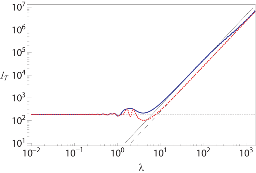
Figure 2: (Ref. [Asatryan10a, ], color online) Transmission length $l_{T}$ vs $\lambda$ for M-stack (thick solid line, direct simulation and calculations based on WSA recurrence relations) and H-stack (thick dashed line, direct simulation). Asymptotics of the localization length $l:$ the short wavelength asymptotic (thin dotted line), and the long wavelength asymptotics—thin solid line for the M-stack and a thin dashed line for the H-stack.

To check the WSA theoretical predictions formulated above we provided a series of numerical calculations. They were made for the lossless stack with uniform distributions of the fluctuations $\delta^{(d)},$ $\delta^{(\nu)}$, with widths of $Q_{\nu}=0.25$ and $Q_{d}=0.2$, respectively and included (a) direct simulations based on the exact recurrence relations (II.19), (II.20); (b) the weak scattering analysis for the transmission length. In all cases, unless otherwise is mentioned, the ensemble averaging is taken over $N_{r}=10^{4}$ realizations.

Throughout this Subsection we considered only M-stacks. Nevertheless, to emphasize the main features of the transmission in metamaterials, compare transmission spectra for a M-stack of $N=10^{5}$ layers and a H-stack of length $N=10^{3}$ plotted in the same Fig. 2. Both stacks are sufficiently long: for the shortest of them parameter $NQ_{\nu}^{2}$ is $62.5\gg 1$. There are two major differences between the results for these two types of samples: first, in the localized regime ($N\gg l_{T}$), the transmission length of the M-stack exceeds or coincides with that of the H-stack; second, in the long wavelength region, the plot of the transmission length of the M-stack exhibits a pronounced bend, or kink, in the interval $\lambda\in[10^{2},10^{3}]$, while there is no such feature in the H-stack results.

Fig. 2 demonstrates an excellent agreement of analytical and numerical results: the curves obtained by direct numerical simulations and by calculations based on the weak scattering approximation (WSA) are indistinguishable (solid line). The short and long wavelength behavior of the transmission length is also in excellent agreement with the calculated asymptotics in both regimes. The characteristic wavelengths of this mixed stack are $\lambda_{1}\approx 148$ and $\lambda_{2}\approx 839$. Therefore, the region $\lambda\lesssim 148$ corresponds to localized regime, whereas longer wavelengths, $\lambda\gtrsim 839$, correspond to the ballistic regime. Thus the kink observed within the region $\lambda_{1}\lesssim\lambda\lesssim\lambda_{2}$ describes crossover from the localized to the ballistic regime. The long wave asymptotic of the ballistic length, as we saw below, coincides with that of reciprocal Lyapunov exponent. Therefore the difference between localization and ballistic lengths of the M-stack simultaneously confirms the difference between localization length and reciprocal Lyapunov exponent in localized regime.

More detail numerical calculations of transmission length, average reflectance, and characteristic wavelengths of the M-stacks with various sizes also demonstrate an excellent agreement between direct simulations and WSA based calculations thus completely confirming the theory presented aboveAsatryan10a .

Until now, we have dealt only with the transmission length $l_{T}(\lambda)$, which was defined through an average value. However, additional information can be obtained from the transmission length $l_{N}(\lambda)$ for a single realization,

$$\frac{1}{l_{N}}=-\frac{\ln\ \left|T_{N}\right|}{N}.$$

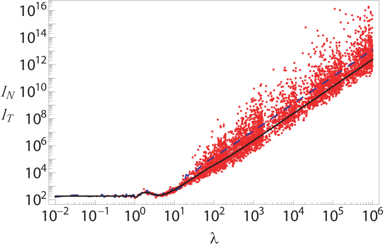
Figure 3: (Ref. [Asatryan10a, ], color online) Transmission lengths $l_{T}$ (solid black line) and the transmission length for a single realization $l_{N}$ (dashed blue line) vs $\lambda$ for a M-stack with $Q_{\nu}=0.25$, $Q_{d}=0.2$ and $N=10^{4}$ layers. Each separate point corresponds to a particular wavelength with its own realization of a random stack.

In the localized regime, i.e. for a sufficiently long M-stack with $N\gg l$, the transmission length for a single realization $l_{N}(\lambda)$ is practically non-random and coincides with $l_{T}(\lambda)$ and $l$, while in the ballistic region it fluctuates. The data displayed in Fig. 3 enables one to estimate the difference between the transmission length $l_{T}(\lambda)$ (solid line) and the transmission length $l_{N}(\lambda)$ for a single randomly chosen realization (dashed line), and the scale of the corresponding fluctuations. Both curves are smooth, coincide in the localized region, and differ noticeably in the ballistic regime. The separate discrete points in Fig. 3 present the values of the transmission length $l_{N}(\lambda)$ calculated for different randomly chosen realizations. It is evident that fluctuations in the ballistic region become more pronounced with increasing wavelength.

III.3 Homogeneous Stack

For an H-stack composed entirely of either normal material or metamaterial layers, the transmission length obtained within the WSA is

$$\frac{1}{l_{T}}=\frac{1}{l}+\frac{1}{N}\times\ \ \ \ \ \ \ \ \ \ \ \ \ \ \ \ \$$

$$\!\!\!\!\mathrm{Re}\left\{\frac{\langle r\rangle^{2}}{(1-\langle t^{2}\rangle)^{2}}\left[1-\mathrm{exp}\left(-\frac{N}{\bar{l}}-i\frac{N}{\bar{l}_{b}}\right)\right]\right\},$$ (III.18)

where $\bar{l}$ is crossover length (III.10) and $\bar{l}_{b}$ is ballistic crossover length defined by equation

$$\frac{1}{\bar{l}_{b}}=-\mathrm{Im}\ln\langle t^{2}\rangle.$$

H-stack localization length $l$ is

$$\frac{1}{l}=-\langle\ln|t|\rangle-\mathrm{Re}\frac{\langle r\rangle^{2}}{1-\langle t^{2}\rangle}$$ (III.19)

where $r,t$ are transmission and reflection coefficients of a $R$ layer (for $L$ layers, they should be replaced by $r^{*}$ and $t^{*}$ however this does not change the final result due to real part operation $\mathrm{Re}$).

Here we consider the simplest lossless model ($\sigma=0$) with only refractive index disorder (i.e., $Q_{d}=0$). In contrast to M-stack case(see Section III.2 below), where a minimal model manifesting all common features of the M-stack transmission properties necessarily includes additional random parameter (in previous Subsection it is layer thickness), for H-stack it is sufficient to include only one such parameter. As earlier, we assume uniform distribution of refractive index fluctuations with the width $2Q_{\nu}$. In this case, the short wave asymptotic of the localization length coincides with that of M-stack (III.12) and similarly to the M-stack, transmission through short H-stacks with $N\lesssim Q_{\nu}^{-2}$ is always ballistic. So below we consider long stacks $NQ_{\nu}^{2}\gg 1$.

In the long wave region $\lambda\gg 1,$ the three characteristic lengths entering Eq. (III.3) asymptotically are

$$l=\displaystyle{\frac{3\lambda^{2}}{2\pi^{2}Q_{\nu}^{2}}},\ \ \ \ \ \ \ \bar{l}=\frac{\lambda^{2}}{8\pi^{2}Q_{\nu}^{2}},\ \ \ \ \ \ \ \ \bar{l}_{b}=\frac{\lambda}{4\pi}.$$ (III.20)

The main contribution to the long wave and short wave asymptotic of the localization length is related to the first term in Eq. (III.19). Thus, the localization length of the H-stack in these two limits is well described by the single scattering approximation. The long wave asymptotic of the H-stack localization length differs from that of M-stack and coincides with that of its reciprocal Lyapunov exponent (III.17) and ballistic length (III.15).

We calculated also H-stack Lyapunov exponent. It is described by the same equation (III.16) as that for M-stack, thus the reciprocal Lyapunov exponents for both types of stacks have the same asymptotic form (III.17). This coincidence was established analytically in a wider spectral region in IMT-10 .

Long H-stacks with $N\gg Q_{\nu}^{{-2}}$ in the long wave region $\lambda\gg 1$ manifest both ballistic and localized behavior. Transition between these regimes is governed by two characteristic wavelengths defined by Eq. (III.11). Similarly to the M-stack case, they are proportional to $Q_{\nu}\sqrt{N},$ differ only by a numerical multiplier and satisfy the inequality $\lambda_{1}(N)<\lambda_{2}(N)$.

At starting part of long wave region $1\ll\lambda\ll\lambda_{1}(N)$ transmission length $l_{T}$ coincides with the localization length $l$ and has asymptotic described by Eq. (III.20). Then after passing transition region $\lambda_{1}(N)\ll\lambda\ll\lambda_{2}(N)$ the ballistic regime $\lambda\gg\lambda_{2}(N)$ starts. In this regime, transmission length coincides with ballistic length $b(\lambda)$ described by equation

$$\frac{1}{b(\lambda)} = \frac{2\pi^{2}Q_{\nu}^{2}}{3\lambda^{2}}\left[1+\frac{NQ_{\nu}^{2}}{12}\left(\frac{\sin\displaystyle{\frac{\lambda_{3}(N)}{2\lambda}}}{\displaystyle{\frac{\lambda_{3}(N)}{2\lambda}}}\right)^{2}\right],$$ (III.21)

$$\lambda_{3}(N)=4\pi N,$$

obtained by expansion of the exponent $\exp\left(-N/\bar{l}\right)$ in Eq. (III.3).

Due to appearance of additional characteristic wavelength $\lambda_{3}(N)$ determined by equation $N=\bar{l}_{b}(\lambda_{3}(N))$ where $\bar{l}_{b}$ is the ballistic crossover length (III.20), ballistic region is naturally divided onto two subregions. The first of them defined by inequalities $\lambda_{2}(N)\ll\lambda\ll\lambda_{3}(N)$ is near ballistic region where ballistic length coincides with localization length

$$b_{n}(\lambda)=\displaystyle{\frac{3\lambda^{2}}{2\pi^{2}Q_{\nu}^{2}}}.$$ (III.22)

Thus crossover from localized regime to ballistic one is not accompanied by any change of transmission length. In the ballistic transition region $\lambda\sim\lambda_{3}(N)$, the second term in Eq. (III.21) becomes essential leading to oscillations of ballistic length. Finally in the far ballistic region $\lambda\gg\lambda_{3}(N),$ expansion of the sine in Eq. (III.21) shows that for long stacks the second term in this equation dominates and far ballistic length is

$$\frac{1}{b_{f}(\lambda)}=\frac{2\pi^{2}Q_{\nu}^{2}}{3\lambda^{2}}\left(1+\frac{NQ_{\nu}^{2}}{12}\right)\approx\frac{N\pi^{2}Q_{\nu}^{4}}{18\lambda^{2}}.$$ (III.23)

The region $\lambda\geq\lambda_{3}(N)$ possesses a simple physical interpretation. Indeed, in this subregion, the wavelength essentially exceeds the stack size and so we may consider the stack as a single weakly scattering uniform layer with an effective dielectric permittivity Asatryan10a

$$\varepsilon_{\mathrm{eff}}=\left(1+\frac{Q_{\nu}^{2}}{3}\right).$$

Substitution this value to the text-book formula for reflectivity of the uniform sample leads immediately to the far long wavelength ballistic length (III.23). We note that because of the effective uniformity of the H-stack in the far ballistic region, the transmission length on a single realization is a less fluctuating quantity than that in the near ballistic region, where it fluctuate strongly as over entire ballistic region for M-stacks.

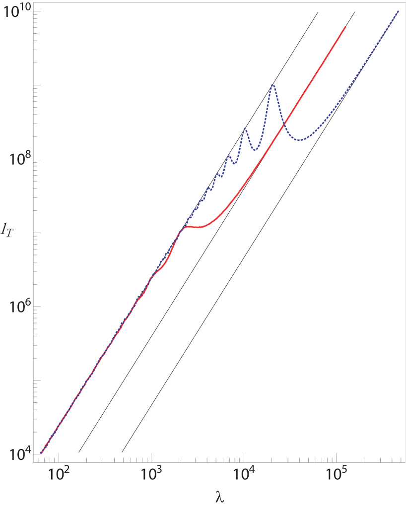
Figure 4: (Ref. [Asatryan10a, ], color online) Transmission length $l_{T}$ vs $\lambda$ for H-stacks of $N=10^{3}$ (solid line), and $10^{4}$ (dotted line) layers (numerical simulation and WSA). Long wave asymptotics for the ballistic length in the near and far ballistic regions are plotted in thin solid lines.

Numerical calculations for H-stack, show an excellent agreement between direct simulations and calculations based on WSA: corresponding curves can not be distinguished. Figure 2 explicitly demonstrates that transmission length preserves the same analytical form in localized long wave region and near ballistic region. For the considered stacks with $N=10^{3}$, the transmission spectrum features corresponding to transition between two ballistic subregions can not be manifested. Indeed, the transition occurs at the wavelength $\lambda\sim 10^{4}$ that is out of range in this figure.

To study the crossover from near to far ballistic behavior, consider the transmission lengths of H-stacks with $N=10^{3}$ and $10^{4}$ over the wavelength range extended up to $\lambda\sim 10^{6}$ plotted in Fig. 4. The transition from the localized to the near ballistic regime occurs without any change in the analytical dependence of transmission length, however the crossover from the near to the far ballistic regime is accompanied by a change in the analytical dependence that occurs at $\lambda=\lambda_{2}(N)$, which for these stacks is of the order of $10^{4}$ and $10^{5}$ respectively. The crossover is accompanied by prominent oscillations described by Eq. (III.21). Finally, we note that the vertical displacement between the moderately long and extremely long wavelength ballistic asymptotes does not depend on wavelength, but grows with the size of the stack, according to the law

$$\ln\frac{b_{n}}{b_{f}}=\ln\frac{NQ_{\nu}^{2}}{12},$$

which stems from Eqs. (III.22), (III.23).

Detailed study of the average reflectivity of the H-stacks with various lengths at all long wave regionAsatryan10a also completely confirm theoretical predictions formulated above.

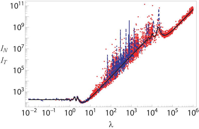
Figure 5: (Ref. [Asatryan10a, ], color online) Transmission lengths $l_{T}$ (solid black line) and the transmission length for a single realization $l_{N}$ (dashed blue line) vs $\lambda$ for a H-stack with $Q_{\nu}=0.25$, $Q_{d}=0.2$ and $N=10^{4}$ layers. Each separate point corresponds to a particular wavelength with its own realization of a random stack.

Consider now statistical properties of the H-stack transmission length on a given realization $l_{N}(\lambda)$. For very long stacks $N\to\infty$ this length becomes practically non-random in both localized region due to self-averaging of Lyapunov exponent, and far ballistic region because due to self-averaging nature of the effective dielectric permittivity. For less long stacks, transmission length $l_{T}$ fluctuates also even in the far ballistic region, however for sufficiently long stacks these fluctuations are essentially suppressed since they must vanish in the limit as $N\to\infty$. This is demonstrated by Fig. 5 where the transmission length $l_{T}$ (solid line) and the transmission length $l_{N}(\lambda)$ for a single randomly chosen realization (dashed line) are plotted. Like the M-stack case, the H-stack single realization transmission length in the near ballistic region is a complicated and irregular function, similar to the well known “magneto fingerprints” of magneto-conductance of a disordered sample in the weak localization regime Altshu . This statement is supported by displayed in Fig. 5 the set of separate discrete points, each of them presenting transmission length calculated for a different randomly chosen realization.

III.4 Transmission Resonances

An important signature of the localization regime is the presence of transmission resonances (see, for example, Refs. Lifshits ; Soven ; Bliokh-2 ), which appears in sufficiently long, open systems and which are the “fingerprints” of a given realization of disorder. These resonances manifest themselves as narrow peaks of transmittivity $|T_{N}|^{2}$ on a given realization as a function of wavelength $\lambda$. Figure 6Asatryan07 presents a single realization of the transmittance $|T_{N}|^{2}$ as a function of $\lambda$ for a M-stack (dashed line) and for the corresponding H-stack of $N=10^{3}$ layers (solid line). It is evident that the resonance properties exhibited by homogeneous and mixed media, serve as another (in addition to the behavior of the localization length) discriminating characteristic of these two media. Indeed there are no resonances for the M-stack for $\lambda\gtrsim 4$, while the disordered homogeneous stack exhibits well pronounced resonances over the entire spectrum.

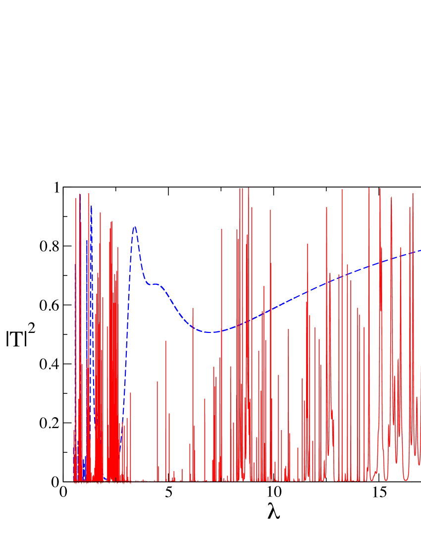
Figure 6: (Ref. [Asatryan07, ], color online) Transmittance $|T|^{2}$ vs $\lambda$ for a single realization ($Q=0.25$, $N=10^{3}$). Solid: normal H-stack, dotted: M-stack.

Note that the dotted curve in Fig. 6 describes resonance properties of periodic $Q_{d}=0$ comparatively short M-stack with only refractive index disorder (RID). Important feature of such a stack is the lack of phase accumulation over its total length: in the particular realization of Fig. 6, the accumulated phase of the wave in the mixed stack never exceeds $\pi/2$. Therefore to subdue such a suppression of the phase accumulation, one need or to enlarge essentially the stack size, or to switch on an additional (thickness $Q_{d}$ or magnetic permittivity $\mu$) disorder.

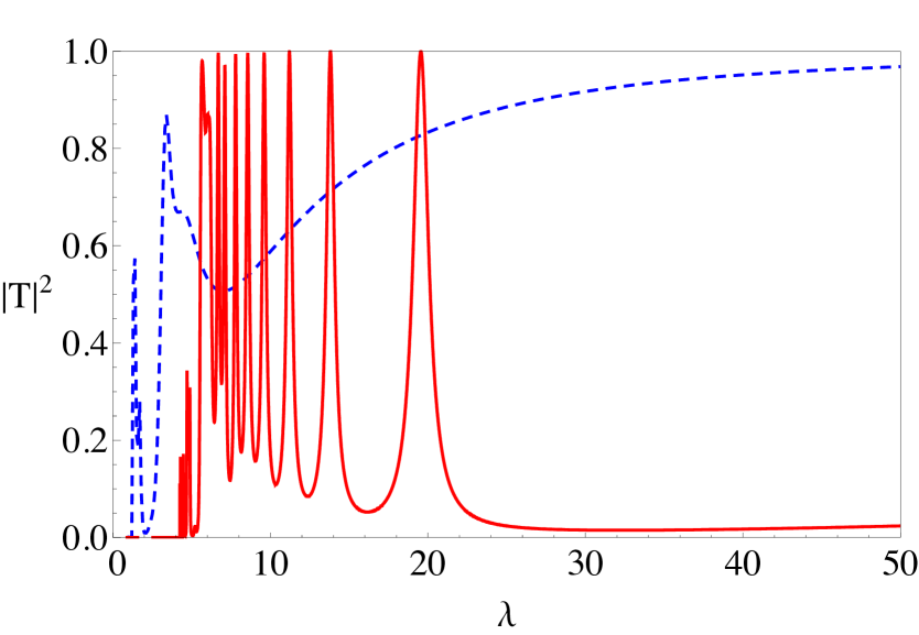
Figure 7: (Ref. [Asatryan10a, ], color online) Single realization transmittance $|T|^{2}$ vs wavelength $\lambda$ for RID M-stacks with $Q_{\nu}=0.25$ and $Q_{d}=0$ for $N=10^{5}$ layers (solid line) and $N=10^{3}$ layers (dotted line).

The first possibility is demonstrated in Fig 7 where transmittance spectra $|T|^{2}(\lambda)$ for a realization, of two different M-stack with two lengths $N=10^{3}$ and $N=10^{5}$ and only refractive index disorder is displayed. It is readily seen that while the resonances in the shorter stack (dashed line) at $\lambda\geq 5$ do not exist at all, they do appear in the same region for the longer sample (solid line).

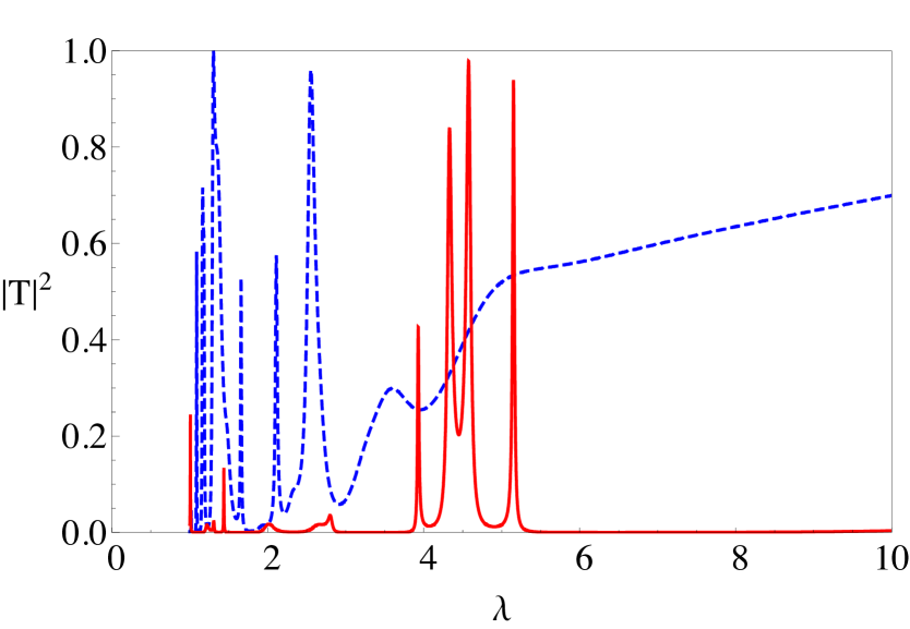
Figure 8: (Ref. [Asatryan10a, ], color online) Single realization transmittance $|T|^{2}$ vs $\lambda$ for M-stack of $N=10^{3}$ layers with $Q_{\nu}=0.25$. Solid line corresponds to an M-stack with $Q_{d}=0.2$, and the dashed line to M-stack with no thickness disorder, i.e., $Q_{d}=0.0$.

The second way to generate transmission resonances is to introduce additional disorder. This is confirmed by the transmittance spectra for a realization, of two M-stacks of the same size $N=10^{3}$ with only refractive index disorder (dashed line), and both (thickness and refractive index) types of disorder (solid line), plotted in Fig. 8. It is clear that while the RID M-stack with this length, is too short to exhibit transmission resonances at $\lambda>3$, resonances do emerge at longer wavelengths for the M-stack with thickness disorder.

Transmission resonances are responsible for the difference between two quantities that characterize the transmission, namely transmittance logarithm $\langle\ln|T|^{2}\rangle$ and logarithm of average transmittance $\ln\langle|T|^{2}\rangle$. The former reflects the properties of a typical realization, while the latter value is often very sensitive to the existence of almost transparent realizations associated with the transmission resonances. Moreover, in some cases namely small number of such realizations contribute mainly to the average transmittance.

Thus the ratio of the two quantities mentioned above

$$s=\frac{\langle\ln|T|^{2}\rangle}{\ln\langle|T|^{2}\rangle}.$$

is a natural characteristic of the transmission resonances. In the absence of resonances, this value is close to unity, while in the localization regime $s>1$. In particular, this ratio takes the value $4$ in the high-energy part of the spectrum of a disordered system with Gaussian white-noise potentialLGP .

Consider the ratio $s(\lambda)$ as a function of the wavelength for RID M- and H-stacks and for the corresponding stacks with thickness disorder plotted in Fig. 9. In all cases, the stack length is $N=10^{3}.$ It is evident that for the RID M-stack $s(\lambda)\approx 1$, i.e.. the length of this M-stack is too short for the localization regime to be realized. In other three cases, however, $s(\lambda)\gtrsim 2$, which means that the localization takes place even in such comparatively short stack.

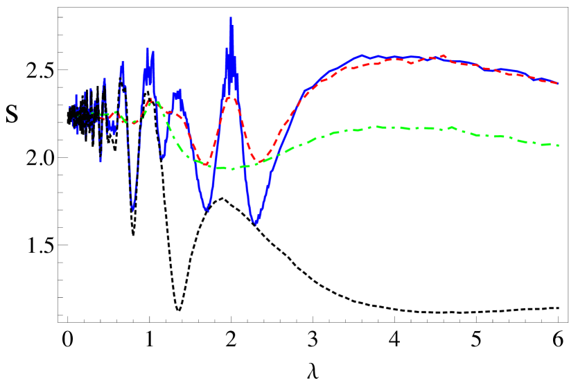
Figure 9: (Ref. [Asatryan10a, ], color online) Ratio $s(\lambda)$ vs. wavelength $\lambda$ for $Q_{\nu}=0.25$ and the stack length $N=10^{3}$. Solid and dashed curves are for the RID H-stack and H-stack with $Q_{d}=0.2$, respectively. The middle dashed-dotted curve is for an M-stack with $Q_{d}=0.25$, and the bottom dotted line is for a RID M-stack.

III.5 Polarization Effects

The results obtained above for normal incidence can be easily generalized to the case of oblique incidence. Here all characteristic lengths and wavelengths depend on angle of incidence $\theta$ and s- and p-polarizations should be considered separately. Qualitatively new features appear: essential enlightening in the vicinity of Brewster angle and appearance of supercritical regime induced by total internal reflection. We describe these new properties within the frameworks of the model defined in the previous Subsection III.1.

General expressions for transmission length for both M-stacks (Eqs. (III.7) - (III.10)) and H-stacks (Eqs. (III.3) - (III.19)) as well as general expressions (III.2) for transmission and reflection coefficients of a single layer remain the same as in the case of normal incidence. However explicit expressions for the parameters entering these coefficients are changed. Fresnel interface reflection coefficient is now given by

$$\rho=\frac{\mathcal{Z}\cos\theta_{\nu}-\cos\theta}{\mathcal{Z}\cos\theta_{\nu}+\cos\theta},$$ (III.24)

$$\mathcal{Z}=\left\{\begin{array}[]{ccc}Z^{-1},&&s-\text{polarization}\\ &&\\ Z,&&p-\text{polarization}.\end{array}\right.$$

Here characteristic angle $\theta_{\nu}$ and the layer impedance $Z$ relative to the background (free space) according Eq. III.4 are

$$\cos\theta_{\nu}=\sqrt{1-\frac{\sin^{2}\theta}{\nu^{2}}},\ \ \ \ Z=\sqrt{\frac{\mu}{\varepsilon}}=\frac{1}{1+\delta_{\nu}}.$$

Then the phase shift $\beta$ is now

$$\beta=kd\nu\cos\theta_{\nu},\ \ \ \ k=2\pi/\lambda.$$ (III.28)

Characteristic angle conserves its direct geometrical meaning for incidence angle $\theta\leq\theta_{c}$ ( subcritical incidence angle) where critical angle is

$$\theta_{c}=\sin^{-1}(1-Q_{\nu}).$$

For the supercritical incidence angle $\theta\geq\theta_{c}$, the values of $\theta_{\nu}$ are complex.

Below we mention only final asymptotical expressions for some characteristic lengths of the problem in the typical cases. We take into account both two types of disorder however in all final results we keep only the leading terms and omit the higher order corrections with respect to the refractive index and thickness fluctuations $Q_{\nu,d}$.

In the short wave limit, localization length is the same for M- and H-stacks. In the subcritical region of incidence angles it is

$$\frac{1}{l}\approx\frac{Q_{\nu}^{2}}{12\cos^{4}\theta}\left\{\begin{array}[]{ccc}1&&s-\text{polarization},\\ &&\\ \cos^{2}2\theta&&p-\text{polarization}.\end{array}\right.$$

Note that for p-polarization, this expression acquires angle dependent multiplier that vanishes at the Brewster angle $\theta=\pi/4$. Accounting for the next term we obtain the localization length at the Brewster angle

$${l}=\frac{45}{4Q^{4}_{\nu}},$$

which is $Q_{\nu}^{-2}$ times larger than that far from the Brewster angle and than that for $s-$polarization in the same shortwave limit.

At the incidence angle $\theta>\theta_{c}$, total internal reflection occurs and the WSA fails. If the supercriticality $\theta-\theta_{c}$ is not extremely small, then the exponent $2i\beta$ in Eq. (III.2) is real and negative and thus the magnitude of the single layer transmission coefficient is exponentially small. This results in the attenuation length for both polarizations

$$\frac{1}{l_{att}}=\mathrm{Im}\langle\beta\rangle=k\ \mathrm{Im}\langle d\sqrt{\sin^{2}\theta-\nu^{2}}\rangle=$$

$$\!\!\!\!\frac{k\sin^{2}\theta}{8Q_{\nu}}(\pi-2\theta_{0}-\sin 2\theta_{0}),\ \ \ \sin\theta_{0}=\frac{\sin\theta_{c}}{\sin\theta}.$$

Due to $\propto k$ dependence, in the short wave limit $l_{att}\to\infty$ and transmission length in supercritical region of the angles of incidence coincides with the attenuation length. However for the same reason at long waves attenuation contribution can be neglected and the main contribution to the transmission length is due to Anderson localization.

In the long wave region, H- and M-stacks demonstrate different behavior and we describe them separately.

a) Homogeneous stacks.
For s-polarization, long wave asymptotic of the transmission length is similar to that for normal incidence (III.21)

$$\frac{1}{l_{T}}=\frac{2\pi^{2}Q_{\nu}^{2}}{3\lambda^{2}\cos^{2}\theta}\times\ \ \ \ \ \ \ \ \$$

$$\left[1+\frac{NQ_{\nu}^{2}}{12}\left(\frac{\sin\displaystyle{\frac{2\pi N\cos\theta}{\lambda}}}{\displaystyle{\frac{2\pi N\cos\theta}{\lambda}}}\right)^{2}\right].$$

This expression describes localized region as well as both ballistic subregions.

In the case of $p-$polarized wave, the localization length is given by

$$\frac{1}{l}=\frac{2\pi^{2}Q_{\nu}^{2}\cos^{2}2\theta}{3\lambda^{2}\cos^{2}\theta}+\frac{\pi^{2}Q_{\nu}^{4}}{6\cos^{4}\theta}\times$$

$$\left(1-\frac{19}{6}\cos 2\theta+\frac{7}{15}\cos 4\theta+\frac{19}{30}\cos 6\theta\right).$$

At Brewster angle $\theta=\displaystyle{\frac{\pi}{4}}$ the first term vanishes and transmission length is

$$\frac{1}{l}=\frac{16\pi^{2}Q^{4}_{\nu}}{45\lambda^{2}}.$$ (III.29)

b) Mixed stacks.
Reciprocal transmission length for $s$-polarized wave is

$$\frac{1}{l_{T}} = \frac{k^{2}Q^{2}_{\nu}}{3\cos^{2}\theta}\left(\frac{1}{2}-\frac{1-f(N\alpha_{s})}{3+\zeta\cos^{4}\theta}\right),$$

$$\alpha_{s} = \frac{k^{2}Q^{2}_{\nu}}{3\cos^{2}\theta}(3+\zeta\cos^{4}\theta),$$ (III.30)

where the function $f$ and parameter $\zeta$ are defined in Eqs. (III.8) and (III.2) correspondingly. Equation (III.5) describes the transition from localization to ballistic propagation at long wavelengths. In the limit $N\to\infty$ transmission length tends to localization length

$$l=\frac{3\lambda^{2}\cos^{2}\theta}{2\pi^{2}Q^{2}_{\nu}}\ \frac{3+\zeta\cos^{4}\theta}{1+\zeta\cos^{4}\theta},$$

while the opposite extreme, i.e., as $N\to 0$, gives the ballistic length

$$b=\frac{3\lambda^{2}\cos^{2}\theta}{2\pi^{2}Q^{2}_{\nu}},$$

which coincides with that for a H-stack in s-polarization.

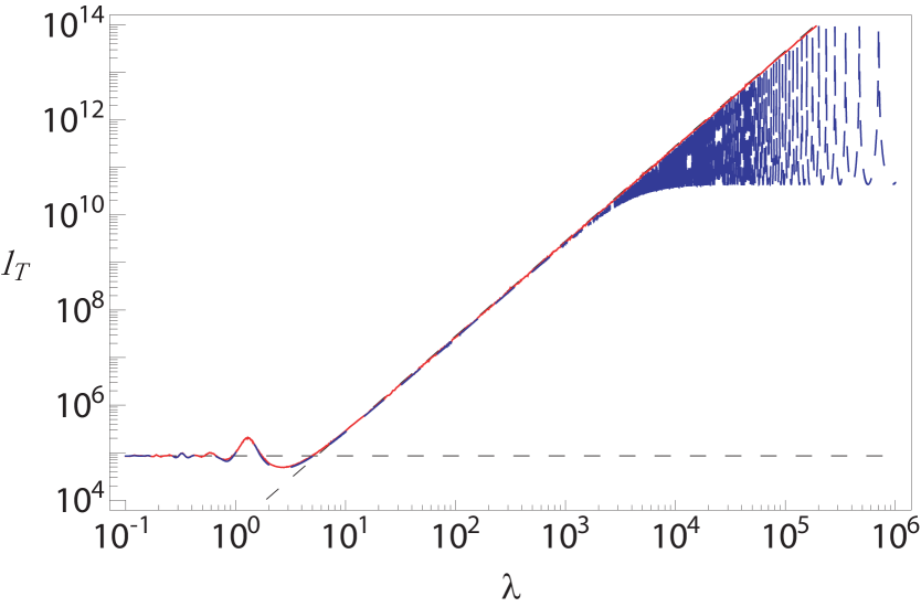
Figure 10: (Ref. [Asatryan10b, ], color online) Transmission length $l_{T}$ versus $\lambda$ for a M- stack in $p$-polarized light with $Q_{\nu}=0.1$, $Q_{d}=0.2$ and $N=10^{6}$, at the Brewster angle $\theta=45^{0}$ red solid line. The blue dashed line shows results for s-polarization and a H-stack, re-plotted for comparison.

For p-polarized waves incident at angles away from the Brewster angle, the transmission length is given by:

$$\frac{1}{l_{T}}=\frac{k^{2}Q^{2}_{\nu}\cos^{2}2\theta}{3\cos^{2}\theta}\times\ \ \ \ \ \$$

$$\left(\frac{1}{2}-\frac{1-f(N\alpha_{p})}{2+\cos^{2}2\theta+\zeta\cos^{4}\theta}\right),$$ (III.31)

$$\ \ \ \ \ \ \alpha_{p}=\frac{k^{2}Q^{2}_{\nu}}{3\cos^{2}\theta}(2+\cos^{2}2\theta+\zeta\cos^{4}\theta).$$

The localization length is deduced from Eq. (III.5) by taking the limit as $N\rightarrow\infty$

$$l=\frac{3\lambda^{2}\cos^{2}\theta}{2\pi^{2}Q^{2}_{\nu}\cos^{2}2\theta}\frac{2+\cos^{2}2\theta+\zeta\cos^{4}\theta}{\cos^{2}2\theta+\zeta\cos^{4}\theta}.$$

Correspondingly, the ballistic length is obtained by calculating the limit as $N\rightarrow 0$

$${b}=\frac{3\lambda^{2}\cos^{2}\theta}{2\pi^{2}Q^{2}_{\nu}\cos^{2}2\theta}.$$

At the Brewster angle $\theta=\pi/4$, accounting for the higher order corrections to r.h.s. of Eq. (III.5) we obtain the transmission length the same result (III.29) that for H-stack.

All analytical predictions are confirmed by numerical calculations. As in the case of normal incidence theoretical curves based on WSA approximations mostly can not be distinguished from those obtained by direct simulations. The results obtained mostly similar to those of normal incidence. Therefore here we mention only some of them which differ from presented above.

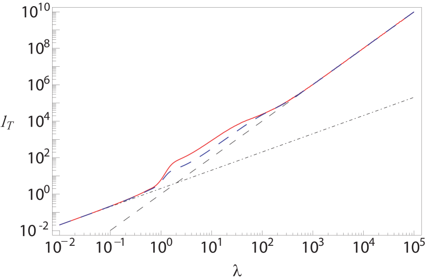
Figure 11: (Ref. [Asatryan10b, ], color online) Transmission length $l_{T}$ versus $\lambda$ for a M-stack in $s$-polarized light with $Q_{\nu}=0.1$, $Q_{d}=0.2$ and $N=10^{4}$, and for the supercritical incidence angle $\theta=75^{\circ}$. Red solid curve: numerical simulations; Blue dash curve: analytic form.

In Fig. 10 the transmission length spectrum of an M-stack of length $N=10^{6}$ in p-polarized light with other parameters $Q_{\nu}=0.1$, $Q_{d}=0.2$, $N_{r}=10^{4}$, and the incidence angle $\theta=\pi/4$ is displayed. The chosen angle of incidence is less than the critical angle $\theta_{c}=\arcsin 0.9=64.16^{\circ}$ and coincides with the Brewster angle for the single layer with mean refractive index $\nu=\pm 1$. The results of the numerical simulation and the WSA analytical forms coincide and are displayed by a single red solid line. Localization occurs for $\lambda\leq\lambda_{1}\approx 19$, while the transition from localization to ballistic propagation occurs at $\lambda\sim\lambda_{1}$. In contrast to the case of s-polarization, this transition is not accompanied by a change of scale and is given by the same wavelength dependence. Transition from near to far ballistic length is accompanied by oscillations of transmission length which are much more pronounced in comparison to the case of normal incidence.

Consider now a supercritical case where the angle of incidence $\theta=75^{\circ}$ exceeds the critical angle. In Fig. 11 we present the transmission length spectrum for s-polarized light is presented. The results of both the exact numerical calculation (red solid line) and the analytic form (long dashed blue curve) are displayed. The short wave (dashed dotted line) and the long wave (black dashed line) asymptotic of the transmission length, respectively coincide with the numerical results for $\lambda\leq 1$ and $200\leq\lambda$. In the intermediate region $1\leq\lambda\leq 200$, however, the theoretical description underestimates the actual transmission length since the WSA is no longer valid for the chosen, supercritical angle of incidence. For p-polarization, the results are qualitatively the same, but with the discrepancy at the intermediate wavelengths even more pronounced.

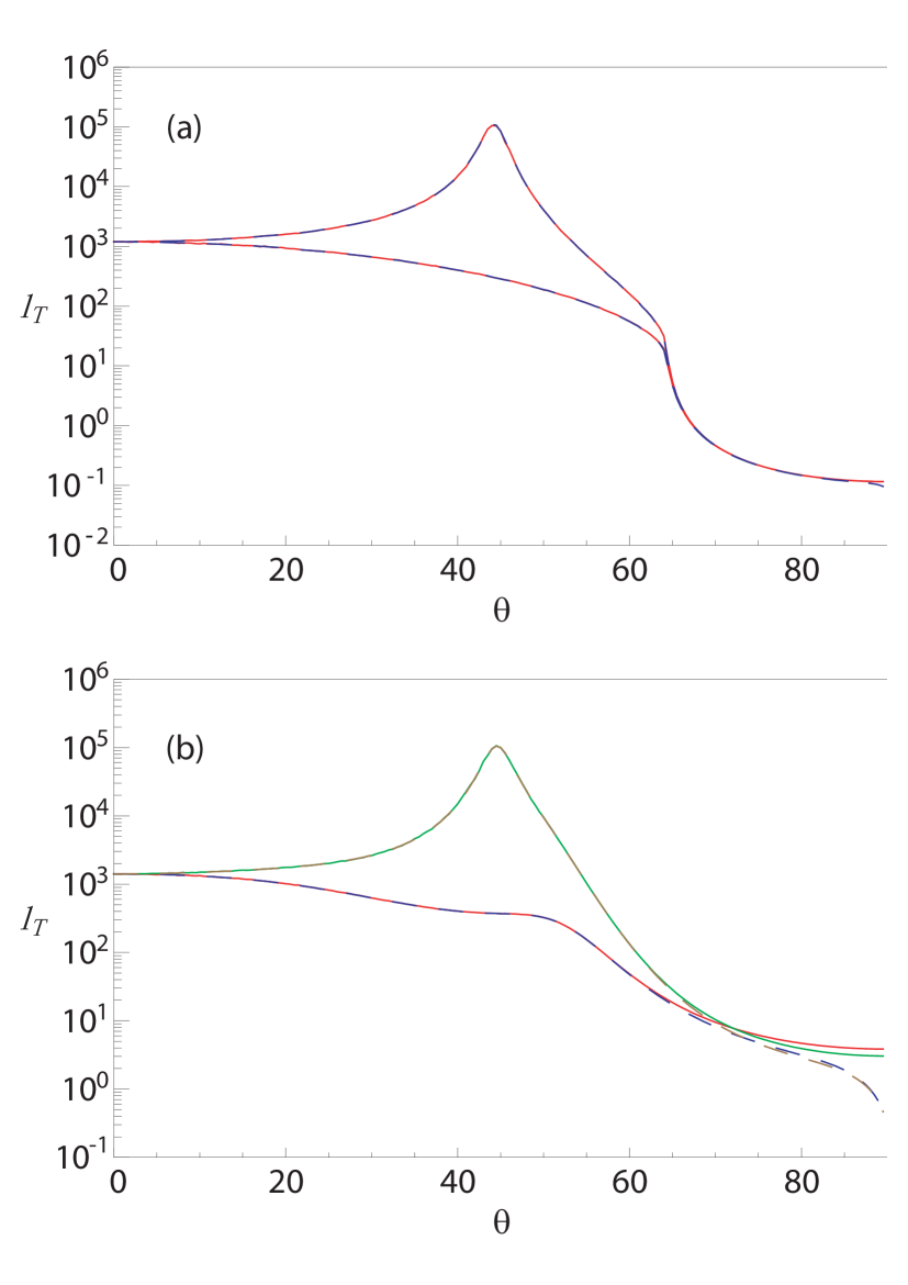
Figure 12: (Ref. [Asatryan10b, ], color online) Transmission length $l_{T}$ versus incidence angle $\theta$ for a mixed stack with $Q_{\nu}=0.1$, $Q_{d}=0.2$, for (a) $\lambda=0.1$ (upper panel), and (b) $\lambda=1$ (lower panel). The top and bottom curves are respectively for p- and s-polarizations.

We consider also the angular dependence of the transmission length for mixed stacks. In Fig. 12 the transmission length $l_{T}$ as a function of the angle $\theta$ for a stack of length $N=10^{6}$ at the two wavelengths $\lambda=0.1$ and $\lambda=1$ is displayed. In either case, the calculated transmission length does not exceed the stack length and so, for subcritical angles, our calculations display the true localization length. For the shorter wavelength $\lambda=0.1$, the form of the transmission length for both polarizations is similar to that observed for homogeneous stacks.

Fig. 12(b) displays results for an intermediate wavelength $\lambda=1$ with the lower solid red and blue dashed curves respectively displaying the results of numerical simulations and analytical predictions for s-polarization, (bottom curves), while the upper solid green and brown dashed curves display simulations and analytical predictions for p-polarization. The agreement between simulations and the theoretical form is again excellent for angles of incidence less then the critical angle, $\theta<\theta_{c}$, while for angles greater then the critical angle, the discrepancies that are evident are again explicable by the breaking down of the WSA at extreme angles of incidence.

III.6 Dispersive Metamaterials

Real metamaterials always are dispersive materials. Here we consider a dispersive model of the stack composed of metalayers with the same thickness $d$ and random dielectric permittivity and the magnetic permeability described by Lorentz oscillator model

$$\varepsilon(f) = 1-\frac{f_{ep}^{2}-f_{e}^{2}}{f^{2}-f_{e}^{2}+i\gamma f},$$ (III.32)

$$\mu(f) = 1-\frac{f_{mp}^{2}-f_{m}^{2}}{f^{2}-f_{m}^{2}+i\gamma f}.$$ (III.33)

Here $f$ is circular frequency, $f_{m}$ and $f_{e}$ are the resonance frequencies and $\gamma$ is the phenomenological absorption parameter. In this model, disorder enters the problem through random resonance frequencies so that

$$f_{e}=\bar{f}_{e}(1+\delta_{e}),\ \ \ \ f_{m}=\bar{f}_{m}(1+\delta_{m}),$$

where $\bar{f}_{e,m}=\langle f_{e,m}\rangle$ are the mean resonance frequencies (with the angle brackets denoting ensemble averaging) and $\delta_{e,m}$ are independent random values distributed uniformly in the ranges $[-Q_{e,m},Q_{e,m}]$. The characteristic frequencies $f_{mp}$ and $f_{ep}$ are non-random. Therefore, in lossless media ($\gamma=0$), both the magnetic permeability and the dielectric permittivity vanish with their mean values, $\bar{\varepsilon}(f)=\langle\varepsilon(f)\rangle$ and $\bar{\mu}(f)=\langle{\mu}(f)\rangle,$ at frequencies $f=f_{ep}$ and $f=f_{mp}$ respectively, i.e.,

$$\mu(f_{mp})=\bar{\mu}(f_{mp})=0,\ \ \ \ \varepsilon(f_{ep})=\bar{\varepsilon}(f_{ep})=0.$$

Following Ref. Shelby ; Smith2010 , in our numerical calculations we choose the layer thickness $d=0.003$m and the values of characteristic frequencies $f_{mp}=10.95\text{GHz}$, $f_{m0}=\bar{f_{m}}=10.05\text{GHz}$, $f_{ep}=12.8\text{GHz}$, $f_{e0}=\bar{f_{e}}=10.3\text{GHz,}$ and $\gamma=10\text{MHz,}$ which fit the experimental data given in Ref. Shelby . That is, we are using a model based on experimentally measured values for the metamaterial parameters. Then we choose the maximal widths of the distributions of the random parameters $\delta_{e,m}$ as $Q_{e,m}=5\times 10^{-3}$ corresponding to weak disorder.

We focus our study on the frequency region $10.40\text{GHz}<f<11.00\text{GHz}$. In the absence of absorption and disorder, for these frequencies the dielectric permittivity and the magnetic permeability of the metamaterial layers vary over the intervals $-26.9<\varepsilon<-2.9$ and $-1.64<\mu<0.055$. The refractive index is negative in the frequency range $10.40\text{GHz}<f<f_{mp}=10.95\text{GHz}$, as shown in the inset of Fig.13. However, at $f_{mp}=10.95\text{GHz}$, the magnetic permeability changes sign and the metamaterial changes from being double negative (DNM) to single negative (SNM). As we show later, such changes have a profound effect on the localization properties.

We study the transmission of a plane wave either s - or p - polarized and incident on a random stack from free space with an angle of incidence $\theta_{0}$.

In the previous Subsections, we have described and used an effective WSA method developed and elaborated in Refs Asatryan07 ; Asatryan10a ; Asatryan10b , for studying the transport and localization in random stacks composed of the weakly reflecting layers.

In the dispersive case, the reflection from a single layer located in free space is not necessarily weak, in which instance the method seems inapplicable. However, we can replace each layer by the same layer surrounded by infinitesimally thin layers of a background medium with permittivity and permeability given by the mean values of $\bar{\varepsilon}(f)\equiv\langle\varepsilon(f)\rangle$ and $\bar{\mu}(f)\equiv\langle\mu(f)\rangle$ respectively. In the considered case of weakly disordered stacks, we can use the WSA approximation for all layers beside two ”leads” connecting the stack with free space from the very left and the very right its ends. The localization characteristics which are intrinsic properties of the stack do not feel the leads. Their role is restricted by only change the coupling conditions to the random stack through the angle of incidence transforming it from its given value $\theta_{0}$ outside the lead to the frequency dependent refracted value $\theta_{b}$ inside the lead. These angles are related by Snell law $\sin\theta_{0}=\sin\theta_{b}\sqrt{\bar{\varepsilon}(f)\bar{\mu}(f)}.$ It is important to note that, while in the localized regime the input and output leads are of no significance, they do play a crucial role when localization breaks down (see below).

The single layer scattering is described by Eqs. (III.2) where according Eqs. (III.1) and(III.28)

$$\beta_{n}=kd\nu_{n}\cos\theta_{n},\ \ \ \nu_{n}=\sqrt{\varepsilon_{n}\mu_{n}},$$ (III.34)

and $k=\displaystyle{\frac{2\pi}{\lambda}=\frac{2\pi f}{c}}$ is the free space wave number. The interface Fresnel reflection coefficient $\rho_{n}$ is given by

$$\rho_{n}=\frac{Z_{b}\cos\theta_{b}-Z_{n}\cos\theta_{n}}{Z_{b}\cos\theta_{b}+Z_{n}\cos\theta_{n}},$$ (III.35)

The impedances $Z_{b}$ and $Z_{n}$ are

$$Z_{b} = \left\{\begin{array}[]{ccc}\sqrt{\bar{\mu}/\bar{\varepsilon}}&&p\text{-polarization},\\ &&\\ \sqrt{\bar{\varepsilon}/\bar{\mu}}&&s\text{-polarization},\\ &&\end{array}\right.,$$

$$Z_{n} = \left\{\begin{array}[]{ccc}\sqrt{\mu_{n}/\varepsilon_{n}}&&p\text{-polarization},\\ &&\\ \sqrt{\varepsilon_{n}/\mu_{n}}&&s\text{-polarization}.\\ &&\end{array}\right.,$$

and the angles $\theta_{b}$ and $\theta_{n}$ satisfy Snell’s law

$$\nu_{n}\sin\theta_{n}=\bar{\nu}\sin\theta_{b} = \sin\theta_{0},\ \ \ \ \bar{\nu}=\sqrt{\bar{\varepsilon}\bar{\mu}}.$$ (III.38)

General WSA expressions (III.19) and (III.9) for localization length of mono-type and mixed stacks remain valid for the stacks composed of dispersive stacks. To study localization properties of such stacks we should insert there the same single layer scattering coefficients (III.2) with dispersive phase shift (III.34) and Fresnel coefficient (III.35).

Dispersion affects essentially the transport properties of the disordered medium. In particular, it can lead to suppression of the localization either at some angle of incidence, or at a selected frequency, or even in a finite frequency range. Below we consider the two first cases for the H-stack composed of $L$-layers. The third case will be considered further in Section III.7.

In the presence of dispersion, the long-wave asymptotic of the localization length is

$$\frac{1}{l}\!=\!\frac{\pi^{2}d^{2}}{2\lambda^{2}(f)}\!\left(\frac{\langle\mu^{2}\rangle-\langle\mu\rangle^{2}}{\langle\mu\rangle^{2}}\!+\!\frac{\langle\varepsilon^{2}\rangle-\langle\varepsilon\rangle^{2}}{\langle\varepsilon\rangle^{2}}\right),$$ (III.39)

where $\mu$ and $\varepsilon$ are given by Eqs. (III.33), (III.32), and frequency-dependent wavelength in the medium

$$\lambda(f)=\frac{c}{f\sqrt{\varepsilon(f)\mu(f)}}.\ \ \ \$$

and can be large even when the wavelength of the incident signal, $\lambda=\displaystyle{\frac{c}{f}},$ is small.

Accordingly, the inverse localization length

$$l^{-1}\propto f^{2}\varepsilon(f)\mu(f)$$

becomes small not only at low frequencies $f\rightarrow 0$ but also in the vicinity of $\mu$- or $\varepsilon$- zero points. For example, as the frequency approaches the $\mu$-zero point from below, i.e., $f\rightarrow f_{mp}^{-}$, in a H-stack of metamaterial layers, $\mu(f)$, for any realization, is proportional to the difference $(f_{mp}-f)$ and the expression for localization length diverges as $(f_{mp}-f)^{-1}$. Formally, this divergence can be treated as delocalization, however the limiting value $1/l=0$ means nothing but the absence of exponential localization. Moreover, when the localization length becomes larger than the size of the stack, ballistic transport occurs and the transmission coefficient is determined by transmission length, rather than by the localization length.

To calculate the transmission coefficient for this case we consider, for the sake of simplicity, a stack with only $\varepsilon$-disorder. Here the transfer matrix of the $n$-th layer at $f=f_{mp}$ has the form

$$\mathcal{T}_{n}\equiv\mathcal{T}(\epsilon_{n})=\left\|\begin{array}[]{ccc}1+\epsilon_{n}&&\epsilon_{n}\\ -\epsilon_{n}&&1-\epsilon_{n}\end{array}\right\|,$$

where $\epsilon_{n}=ikd\varepsilon_{n}/2.$

As a consequence of the easily verified group property

$$\mathcal{T}(\epsilon_{1})\mathcal{T}(\epsilon_{2})=\mathcal{T}(\epsilon_{1}+\epsilon_{2}),$$

it follows that the stack transfer matrix $\mathcal{T}$ is

$$c\mathcal{T}=\prod_{n=1}^{N}\mathcal{T}(\epsilon_{n})=\left\|\begin{array}[]{ccc}1+\mathcal{E}&&\mathcal{E}\\ &&\\ -\mathcal{E}&&1-\mathcal{E}\end{array}\right\|,$$

where

$$\mathcal{E}=\frac{ikL}{2}\frac{1}{N}\sum_{n=1}^{N}\varepsilon_{n},\ \ \ \ \ L=Nd.$$

In a sufficiently long stack, $\mathcal{E}\approx\frac{1}{2}ikL\bar{\epsilon}$ and the transmittance T$=\left|\mathcal{T}_{11}\right|^{-2}$ is given by

$$\text{T}=\frac{1}{1+\left(\displaystyle{\frac{kL\bar{\varepsilon}(f)}{2}}\right)^{2}}.$$

Thus, at the frequency $f_{mp}$, the transmittance of the sample is not an exponentially decreasing function of the length $L$ (as is typical for 1D Anderson localization). It decreases much more slowly, namely, according to the power law $\text{T}\propto L^{-2}$. The explanation of such a decrease is that at a $\mu$-zero point ($f=f_{mp}$), the refractive index $\nu_{n}$ vanishes together with the phase shift $\beta_{n}=kd\nu_{n}\cos\theta_{n}$ across the layer, thereby destroying the interference, which is the main cause of localization. Another form of the explanation is that the effective wavelength inside the stack tends to infinity when $\mu\rightarrow 0$ and exceeds the stack length. Obviously, such a wave is insensitive to disorder and therefore cannot be localized.

In the limit as the frequency approaches the $\mu$-zero frequency, from above, i.e., $f\rightarrow f_{mp}^{+}$, the medium is single-negative and $\varepsilon\mu<0$. For frequencies $f$ not too close to $f_{mp},$ the radiation decays exponentially inside the sample due to tunneling, and in the absence of dissipation the decay rate is:

$$l_{att}=\frac{1}{kd\sqrt{-\langle\mu\rangle\langle\varepsilon\rangle}}.$$ (III.40)

Thus, as we approach the $\mu$-zero frequency from the right, the formally-calculated localization length diverges as $l\propto(f-f_{mp})^{-1/2}$ i.e. much more slowly than for the left-hand limit for which $l\propto(f_{mp}-f)^{-1}.$ The transport properties in the vicinity of the $\varepsilon$-zero frequency $f_{ep}$ can be considered in a similar manner. Waves are also delocalized in the more exotic case when both dielectric permittivity and magnetic permeability vanish simultaneously. The vanishing of both $\mu$ and $\varepsilon$ simultaneously can happen at Dirac points in photonic crystals Hu .

The use of off-axis incidence from free space for frequencies for which $\mu$ or $\varepsilon$ are zero is not an appropriate mechanism for probing the suppression of localization. In such circumstances, tunneling occurs and the localization properties of the stack are not “accessible” from free space. Nevertheless, suppression of localization can be revealed using an internal probe, e.g., by placing a plane wave source inside the stack, or by studying the corresponding Lyapunov exponent. Both approaches show total suppression of localization at the frequencies at which dielectric permittivity or magnetic permeability vanish.

In such circumstances, each layer which is embedded in a homogeneous medium with material constants given by the average values of the dielectric permittivity and magnetic permeability, is completely transparent, with this manifesting the complete suppression of localization. However the “delocalized” states at the zero-$\mu$ or zero-$\varepsilon$ frequencies are in a sense trivial, corresponding to fields which do not change along the direction normal to the layers.

Another example of the suppression of localization is related to the Brewster anomaly. As we saw above, in a non-dispersive mixed stack with only thickness disorder, delocalization of $p$-polarized radiation occurs at the Brewster angle of incidence. At this angle, the Fresnel coefficient $\rho$ (III.24) and, therefore, the reflection coefficient (III.2) as well, vanish for any frequency, thus making each layer completely transparent.

In the presence of dispersion, the same condition $\rho=0$ leads to more intriguing results. In this instance, frequency-dependent angles, at which a layer becomes transparent, exist not only for $p$-polarization, but also for an $s$-polarized wave. This means that the Brewster anomaly occurs for both polarizations, with the corresponding angles, $\theta_{p}$ and $\theta_{s},$ being determined by the conditions

$$\tan^{2}\theta_{p} = \frac{\varepsilon(\varepsilon\overline{\mu}-\overline{\varepsilon}\mu)}{\overline{\varepsilon}(\varepsilon\mu-\overline{\varepsilon}\,\overline{\mu})},$$ (III.41)

$$\tan^{2}\theta_{s} = \frac{\mu(\overline{\varepsilon}\mu-\varepsilon\overline{\mu})}{\overline{\mu}(\varepsilon\mu-\overline{\mu}\,\overline{\varepsilon})}.$$ (III.42)

The right hand sides of these equations always have opposite signs. Therefore from Brewster conditions (III.41) and (III.42) one can find either the Brewster angle and corresponding polarization for a given frequency, or the Brewster frequency and corresponding polarization for a given angle of incidence.

While, for a stack with only thickness disorder, the condition $\rho=0$ can be satisfied for all layers simultaneously, when $\varepsilon$ and/or $\mu$ fluctuate, the conditions (III.41) or (III.42) define the frequency-dependent Brewster angles which are slightly different for different layers. These angles occupy an interval within which the stack is not completely transparent, but has anomalously large transmission lengths Sipe ; Asatryan10b .

When only the dielectric permittivity is disordered and $\mu=\overline{\mu},$ the Brewster conditions (III.41), (III.42) simplify to

$$\tan^{2}\theta_{s} = -1,$$ (III.43)

$$\tan^{2}\theta_{p} = \frac{\varepsilon}{\overline{\varepsilon}}\approx 1.$$ (III.44)

In this case, the Brewster condition is satisfied only for p-polarization. For weak disorder, the Brewster angle of incidence from the effective medium is $\theta_{p}\approx\pi/4$. For a given frequency $f$, angle of incidence from free space, $\theta_{0}$, should be found from Snell’s law (III.38), and for a given $\theta_{0}$, the Brewster frequency $f_{p}$ follows from

$$\sqrt{\overline{\varepsilon}(f_{p})\overline{\mu}(f_{p})}=\frac{\sin\theta_{0}}{\sin\theta_{p}}=\sqrt{2}\sin\theta_{0}.$$ (III.45)

Note that this equation may be satisfied at multiple frequencies depending on the form of the dispersion.

The case of only magnetic permeability disorder, $\varepsilon=\overline{\varepsilon}$, is described by similar equations which are obtained by replacement $s\leftrightarrow p$ in Eqs. (LABEL:brewSe) - (III.45).

For disorder in both the permeability and the permittivity, the existence of a Brewster anomaly angle depends, in accordance with Eqs. (III.41) and (III.42), on the sign of the quantity $\xi=(\overline{\varepsilon}\mu-\varepsilon\overline{\mu})/(\varepsilon\mu-\overline{\varepsilon}\overline{\mu})$. If $\xi>0$, the Brewster angle exists for $s$-polarization, while if $\xi<0$, it exists for $p$-polarization. In the case $\xi=0$, the layer and the medium in which it is embedded are impedance matched, and thus the layer is completely transparent.

The features of transmission length mentioned above are completely confirmed by numerical calculations. Consider first the case of normal incidence on a stack of $N=10^{7}$ layers, in which we randomize only the dielectric permittivity ($Q_{m}=0$) with $Q_{e}=0.5\times 10^{-2}$. In Fig. 13 the transmission length $l_{T}$ as a function of frequency $f$ is displayed. The upper curves present the lossless case, while the lower curves show the effects of absorption (see Asatryan12 for details).

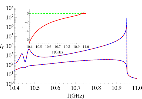
Figure 13: (Ref. [Asatryan12, ], color online) Transmission length $l_{T}$ vs frequency $f$ at normal incidence ($\theta_{a}=0$) for a metamaterial stack without absorption (top curve) and in the presence of the absorption (bottom curves). Red solid curves display numerical simulations while blue dashed curves show the analytical predictions. Inset: the real (red solid line) and imaginary (green dashed line) part of the metamaterial layer refractive index.

The red, solid curves and the blue, dashed curves display results from numerical simulations and the WSA theoretical prediction respectively. The top curves represent the genuine localization length for all frequencies except those in the vicinity of $f\approx f_{mp}=10.95\text{GHz}$ where the transmission length dramatically increases.

In the absence of absorption, for frequencies $f>10.95\text{GHz}$, the metamaterial transforms from being double negative to single negative (see inset in Fig. 13). The refractive index of the metamaterial layer changes from being real to being pure imaginary, the random stack becomes opaque, and the transmission length substantially decreases. Such a drastic change in the transmission length (by a factor of $10^{5}$) might be able to exploited in a frequency controlled optical switch. Across the frequency interval $10.4GHz<f<11.0$GHz, theoretical results are in an excellent agreement with those of direct simulation. Moreover, for all frequencies except in the region $10.4Ghz<f<10.5$GHz, the single scattering approximation excellently describes the $l_{T}$ behavior. Quite surprisingly, the asymptotic equations (III.39) and (III.40) are in the excellent agreement with the numerical results even over the frequency range $10.9\text{Ghz}<f<11.0\text{Ghz}$, including in the near vicinity of the frequency $f_{mp}=10.95\text{GHz}$ at which $\mu$ vanishes.

Absorption substantially influences the transmission length (the lower curve in Fig.13)Asatryan12 and smoothes the non-monotonic behavior of the transmission length for $f<10.5\text{GHz}$. The small dip at $f\approx 10.45\text{GHz}$ correlates with the corresponding dip in the transmission length in the absence of absorption. The most prominent effect of absorption occurs for frequencies just below the $\mu$-zero frequency $f_{mp}=10.95\text{GHz}$. While in the absence of absorption, the stack is nearly transparent in this region, turning on the absorption reduces the transmission length by a factor of $10^{2}$–$10^{3}$ for $f>10.7\text{GHz}$. In contrast, for frequencies $f>10.95\text{GHz}$, the transmission lengths in the presence and absence of absorption are nearly identical because here the stack is already opaque and its transmittance is not much affected by an additional small amount of absorption.

The case where both disorders of the dielectric permittivity and magnetic permeability are present, is qualitatively similar to that of the single disorder case considered above.

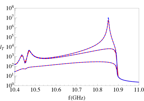
Figure 14: (Ref. [Asatryan12, ], color online) Transmission length $l_{T}$ vs frequency $f$ for $\theta_{a}=30^{\circ}$ for a metamaterial stack: without absorption, p-polarization (top curves), s polarization (middle curves); in the presence of absorption (bottom curves).

In the case of oblique incidence, polarization effects become important. In Fig.14, the transmission length frequency spectrum is displayed for the same metamaterial H-stack with only dielectric permittivity disorder for the angle of incidence $\theta_{0}=30^{\circ}$. Here for frequencies $f<10.55\text{GHz}$, the transmission length is largely independent of the polarization. Moreover it does not differ from that for normal incidence (compare with the top curve in Fig.13 ). This is due to the high values of the refractive indices at these frequencies ($|\nu_{n}|>4)$, resulting in almost zero refraction angles (III.38) for angles of incidence that are not too large.

The transmission length manifests a sharp maximum at an angle close to the Brewster angle, as commented upon in Refs Sipe ; Asatryan10b . This is indeed apparent in Fig. 14 for the frequency $f\approx 10.85\text{GHz}$. Because only $\varepsilon$ fluctuates, the Brewster condition is satisfied only for p-polarization (III.43) at a single frequency $f_{p}\approx 10.852\text{GHz}$. The introduction of additional permeability disorder (not shown) reduces the maximum value of the localization length by two orders of magnitude.

Comparison of Figs 13 and 14 shows that the frequency of the maximal suppression of localization decreases as the angle of incidence increases. At normal incidence it coincides with the $\mu$-zero frequency $f_{mp}$ while for oblique incidence at $\theta_{0}=30^{\circ}$ it coincides with the Brewster frequency $f_{p}$ for p-polarization.

Absorption strongly diminishes the transmission providing the main contribution to the transmission length while the permittivity disorder has little influence on the transmission length. In this case, the results for both two polarizations are therefore practically indistinguishable.

The transmission properties of a stack with only magnetic permeability disorder at oblique incidence, are similar to those for the case of only dielectric permittivity disorder. The key difference is that there is a Brewster anomaly for s-polarization while for p-polarization it is absent.

We consider also the dependence of the transmission length on the angle of incidence at a fixed frequency. The results for both polarizations are displayed in Fig. 15. Here we have plotted the transmission length of the stack with only dielectric permittivity disorder with $Q_{e}=0.5\times 10^{-2}$ at the frequency $f=10.90\text{GHz}$. The upper and middle curves in this figure correspond to the results for $p$- and $s$-polarized waves respectively in the lossless case. For $s$-polarized light, the transmission length decreases monotonically with increasing angle of incidence, while for $p$- polarized wave it increases with increasing angle of incidence. Such behavior reflects the existence of a Brewster angle for $p$-polarization at the Brewster angle $\theta_{0}=20^{\circ}$. The red solid curve shows the results of simulations, while the blue dashed line is the analytic prediction.

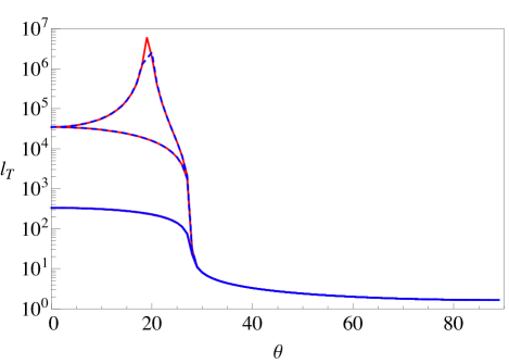
Figure 15: (Ref. [Asatryan12, ], color online) Transmission length $l_{T}$ vs angle of incidence for a homogenous metamaterial stack at $f=10.7\text{GHz}$ with permittivity disorder: in the absence of absorption—upper curve and for $p$ polarization; middle curve is for $s$ polarization and in the presence of absorption and for both polarizations, lower curves.

As in the previous cases, in the presence of absorption, the results for both polarizations are almost identical (the lower curves in Fig. 15). For angles $\theta_{0}<30^{\circ}$, the transmission length is dominated by absorption, while for angles $\theta_{0}>30^{\circ}$ tunneling is the dominant mechanism. The results for permeability disorder are very similar to those for permittivity disorder.

For normal H-stacks, the transmission length manifests exactly the same behavior as for H-stacks comprised of metamaterial layers.

III.7 Anomalous Suppression of Localization

In this Section, we consider the stacks with only refractive index disorder (RID) i.e. the stacks with $\delta_{d}=\delta_{\mu}=0$. In this limit, there is nothing special for H-stacks. Their transmission length demonstrates qualitatively and quantitatively the same behavior as was observed in the presence of both refractive index and thickness disorder. Corresponding formulae for the transmission, localization, and ballistic lengths can be obtained from the general case by taking the limit as $Q_{d}\rightarrow 0$.

In the case of M-stacks, however, the situation changes markedly. Here suppression of localization in the long wave region becomes anomalously large enhancing transmission length on some orders of magnitude and even changing its functional dependence on the wavelengthAsatryan07 . Instead of the universal $\propto\lambda^{2}$ dependence, long wave asymptotic of both localization length $l$ and reciprocal Lyapunov exponent $l_{\xi}$ follows a power law $\propto\lambda^{m}$ with much larger exponent $m.$

Let us start with some numerical results demonstrating such an anomalous growth of the long wave localization lengths $l,\ l_{\xi}$ of the minimally disordered M-stack with only RID. In Fig.16 localization length $l_{\xi}$ for M-stack with $Q=0.25$ is plotted. Solid line in Fig. 16 corresponds to $l_{\xi}$ for the propagation in a M-stack and a single realization of $N=10^{9}$ layers, while the dashed line is for the corresponding H-stack with the same parameters. Within the localization region $l_{\xi}(\lambda)<10^{8}$, M-stack reciprocal Lyapunov exponent grows in the long wave region essentially faster than that of H-stack. While for H-stack is described by standard exponent $m=2$, its value for M-stack was estimated as $m=6$ and the phenomenon itself was named as $\lambda^{6}$ anomaly. The observed anomalous suppression of localization was attributed to a lack of phase accumulation over the sample, due to the cancelation of the phase that occurs in alternating $L$- and $R$-layersAsatryan07 .

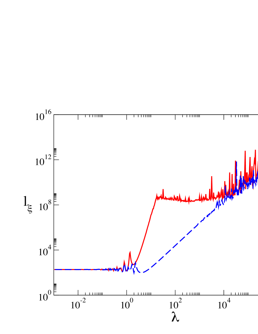
Figure 16: (Ref. [Asatryan07, ], color online) Localization length $l_{\xi}$ vs. wavelength $\lambda$ for $Q=0.25$ and $N=10^{9}$ layers; solid line is for the M-stack, while the dashed line is for the corresponding (normal) H-stack.

Anomalous suppression of localization is manifested also in the case of oblique incidence. The next Figure 17 displays transmission length spectra for a M-stack with only refractive index disorder for an angle of incidence of $\theta=30^{\circ}$. There is a striking difference between the two polarizations: in the case of p-polarized light, there is strong localization at long wavelengths ($\lambda\leq 10^{2}$), with the localization length showing $\propto\lambda^{2}$ dependence. In contrast, the localization length for s-polarized light is much larger and is estimated as $\approx\lambda^{6}$ dependence as occurs for normal incidence. Note that for s-polarization, anomalous enlightening manifests itself only in localization regions in Fig. 17 which are bounded from above by the wavelength limits $\lambda\leq 5,9$, and $12$ for stacks of length $N=10^{5},10^{7}$, and $8\times 10^{8}$ respectively.

This asymmetry between the polarizations suggests that the suppression of localization is due not only to the suppression of the phase accumulation but also to the vector nature of the electromagnetic wave. Because of the symmetry of Maxwell’s equations between the electric and magnetic fields, it is to be expected that for a model in which there is disorder in the magnetic permeability (with $\varepsilon=\pm 1$) the situation will be inverted with anomalous enlightening for p-polarized waves and with s-polarization showing strong localization.

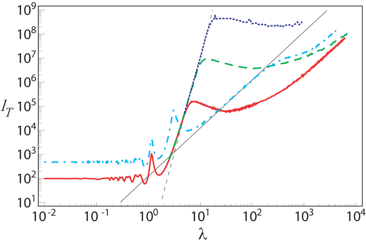
Figure 17: (Ref. [Asatryan10b, ], color online) Transmission length $l_{T}$ versus $\lambda$ for a M-stack with $Q_{\nu}=0.25$, $Q_{d}=0$ and $\theta=30^{0}$ for p-polarized light (cyan dashed dotted curve, $N=10^{6}$) and s-polarized light (red solid curve, $N=10^{5}$; green dashed curve, $N=10^{7}$; blue dotted curve, $N=8\times 10^{8}$).

The results of calculationsAsatryan10a provided for much longer stacks up to $N=10^{12}$ qualitatively completely coincided with the previous ones. However more detailed studies quantitatively occurred slightly different. Generation of a least squares fitting $l_{T}=A\lambda^{m}$ to the transmission length data, led to a bit surprising conclusions. The best fits were $m\approx 6.25$ for $N=10^{7}$, $m\approx 7.38$ for $N=10^{9}$, and even $m\approx 8.78$, for $N=10^{12}.$ This shows that the question about a genuine value of exponent $m$ remains still open.

Consider now the long wave behavior of the localization length in the presence of dispersion. In the panel a) of the Fig.18, the transmission length spectrum is plotted in the case of normal incidence, for a small permittivity disorder of $Q_{e}=0.5\times 10^{-2}$. One can immediately observe significant (up to four orders of magnitude) suppression of localization in the frequency region $10.50\text{GHz}<f<10.68\text{GHz}$. However, this suppression seems to have nothing common with observed above anomalous enlightening. Indeed, in this case the localization length grows with increasing frequency, while in the previous studies Asatryan07 ; Asatryan10a ; Asatryan10b , similar growth has been observed with increasing incident wavelength. This is demonstrated in Fig.18b where the same transmission length spectrum is plotted as a function of free space wavelength. Thus, the localization length decreases by four orders of magnitude, manifesting as an enhancement, rather than the suppression, of localization with increasing wavelength.

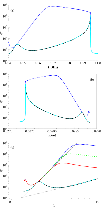
Figure 18: (Ref. [Asatryan12, ], color online) (a)Transmission length $l_{T}$ vs frequency $f$ for a mixed stack with $N=10^{7}$ layers (top dotted blue curve), and only dielectric permittivity disorder. The bottom curves on all panels (a,b,c) are for a stack with $N=10^{7}$ layers with both permittivity and permeability disorder (cyan, solid curve display simulation results while the dashed, black curve is for the analytic prediction; (b) is the same as in (a) but plotted as a function of the free space wavelength $\lambda_{0}$ while on panel (c) we plot the transmission length as a function of the averaged wavelength inside of the stack normalized to the thickness of the layer, for $N=10^{7}$ layers (blue dotted top curve), $N=10^{6}$ layers (dashed green curve) and for $N=10^{5}$ layers (red solid curve) respectively.

Although at the first sight these findings are in sharp contrast with the previous ones, they are correct and physically meaningful. In the model studied earlierAsatryan07 ; Asatryan10a ; Asatryan10b , the wavelength of the incident radiation largely coincided with the wavelength inside each layer. In dispersive medium considered here, these two wavelengths differ substantially. Accordingly, in Fig.18c, we plot the transmission length as a function of wavelength within the stack and obtain results which are very similar to those in Refs. Asatryan07 ; Asatryan10a ; Asatryan10b . To emphasize this similarity, we have plotted the transmission length spectrum for three different stack lengths: $N=10^{5},10^{6},10^{7}$. It is easily seen that the suppression of localization in the dispersive media is qualitatively and quantitatively similar to that predicted in Ref. Asatryan07 . Corresponding exponent $m$ of anomalous enlightening estimated with the help of these results, is $m\approx 8.2$.

Enhanced suppression of localization exists in the strictly periodic alternative M-stacks with a constant layer thickness and only refractive index disorder. By other words, in mixed stacks having constant layer thickness, the dielectric permittivity disorder alone is not sufficiently strong to localize low-frequency radiation by a standard way. There are many ways to violate these conditions. It is possible to add thicknesses fluctuationsAsatryan07 ; Asatryan10a , or magnetic permeability fluctuationsAsatryan12 , or to introduce a weak difference between two constant thicknesses of $R$- and $L$-layers, or not to change any parameter but rearrange randomly the same numbers $N/2$ of $R$- and $L$-layersAsatryan10a . Each such a violation immediately destroys anomalous suppression of localization and restores standard long wave asymptotic $l\propto\lambda^{2}$.

The analytical results obtained above in Section III, survive in the $\delta_{d}\rightarrow 0$ limit and predict $l\propto\lambda^{2}$ asymptotic. However more detailed investigation shows that WA in its form (II.21), (II.22) fails in this limitAsatryan10a .

As was mentioned above, localization length $l_{\xi}$ manifests qualitatively the same behavior as transmission length $l_{T}.$ At the same time, its calculation is simpler than that of $l_{T}$. Lyapunov exponent in minimally disordered M-stacks was calculated inMak-12 using some version of the method described in Refs. [GP ; LGP ; PF ; GMP ] and at the end of Section II.2. The remaining part of this Subsection contains slightly modified details and results of this calculation [Mak-12 ].

Consider the electromagnetic wave of frequency $\omega=ck,$ in infinite array comprised of two types of lossless alternative $\alpha$ and $\beta$ layers of equal dimensionless thickness $\Delta_{j}=1$ with random only dielectric permittivities. Enumerate the layers so that $j$-th layer occupy the interval $j-1\leq z<j$ and choose all odd layers of $\alpha$ type and all even of $\beta$ type. For alternative array, it is natural to choose an elementary cell composed of two adjacent layers, as the main basic element of the arrayAsatryan07 ; Mak-12 . The $n$-th cell occupies interval $2n-2\leq z<2n$ and consists of $(2n-1)$-th and $2n$ layers of type $\alpha$ and $\beta$ correspondingly. Each layer is characterized by its type $\alpha$ ($\beta$), magnetic permeability $\mu_{\alpha}=1$ ($\mu_{\beta}=\pm 1$), refractive index $\nu_{\alpha}(n)$ ( $\nu_{\beta}(n)$), impedance $Z_{\alpha}(n)=1/\nu_{\alpha}(n)$ ($Z_{\beta}(n)=\pm 1/\nu_{\alpha}(n)$), and wave number $k_{\alpha,\beta}=k\nu_{\alpha,\beta}$ of the wave.

Within such a model,two systems are considered: the H-array when both $\alpha$ and $\beta$ layers are made of right-handed materials, and M-array where $\alpha$ layers are right-handed material while $\beta$ layers are of left-handed material. We emphasize that on the contrary of H-stack notion where all the layers have the same statistical properties, H-array is composed of two different materials with different statistical properties for odd and even layers. Disorder is incorporated into the model via dielectric permittivities $\varepsilon_{\alpha,\beta}$ only, so that refractive index $\nu$ is a sole fluctuation parameter and the upper index in its fluctuations $\delta^{(\nu)}_{\alpha,\beta}(n)$ can be omitted

$$\nu_{\alpha}(n)=1+\delta_{\alpha}(n),\ \ \ \ \nu_{\beta}(n)=\pm[1+\delta_{\beta}(n)].$$ (III.46)

Refractive index fluctuations $\delta_{\alpha,\beta}(n)$ are assumed to be delta-correlated with zero mean value $\langle\delta_{\alpha,\beta}(n)\rangle=0$, and variance $\sigma^{2}$,

$$\langle\delta_{\alpha}(n)\delta_{\beta}(n^{\prime})\rangle=\sigma^{2}\delta_{\alpha\beta}\delta_{nn^{\prime}}\,,$$ (III.47)

where angular brackets mean the ensemble average.

To calculate Lyapunov exponent of the electromagnetic wave of the frequency $\omega$, consider two component vector

$$\vec{S}_{n}=\left(\begin{array}[]{c}Q_{n}\\ \\ P_{n}\end{array}\right)$$

with components

$$Q_{n}=E(2n-2),\ \ \ P_{n}=\frac{c}{\omega}E^{\prime}(2n-2)$$ (III.48)

proportional to the field and its derivative at the left edge of the $n$-th cell. These components are real. Therefore they automatically correspond to the currentless field and can be parametrized as

$$\vec{S}_{n}=e^{\xi_{n}}\left(\begin{array}[]{c}\cos\theta_{n}\\ \\ \sin\theta_{n}\end{array}\right)$$ (III.49)

(compare with Eq. (II.12)). Note that this is currentless state in the basis of standing waves while in Section II.2 the basis of running waves was used.

Using Maxwell equations and appropriate boundary conditions on the interfaces of the layers, one obtains dynamic equation

$$\vec{S}_{n+1}=\hat{T}\vec{S}_{n}.$$ (III.50)

Here $\hat{T}_{n}$ is the unimodular matrix with elements

$$\begin{array}[]{ccc}T_{11}&=&\cos\varphi_{\alpha}\cos\varphi_{\beta}-Z_{\alpha}^{-1}Z_{\beta}\sin\varphi_{\alpha}\sin\varphi_{\beta},\\ T_{12}&=&Z_{\alpha}\sin\varphi_{\alpha}\cos\varphi_{\beta}+Z_{\beta}\cos\varphi_{\alpha}\sin\varphi_{\beta},\\ T_{21}&=&-Z_{\alpha}^{-1}\sin\varphi_{\alpha}\cos\varphi_{\beta}-Z_{\beta}^{-1}\cos\varphi_{\alpha}\sin\varphi_{\beta},\\ T_{22}&=&\cos\varphi_{\alpha}\cos\varphi_{\beta}-Z_{\alpha}Z_{\beta}^{-1}\sin\varphi_{\alpha}\sin\varphi_{\beta}\end{array}.$$ (III.51)

They depend on the cell number $n$, due to randomized refractive indices (III.46) entering both the impedances $Z_{\alpha,\beta}(n)$ and phase shifts $\varphi_{\alpha,\beta}(n)$,

$$\varphi_{\alpha}(n) = \frac{1}{2}k_{\alpha}(n)=\varphi[1+\delta^{\nu}_{\alpha}(n)],$$

$$\varphi_{\beta}(n) = \frac{1}{2}k_{\beta}(n)=\pm\varphi[1+\delta^{\nu}_{\beta}(n)],$$

with $$\varphi=k/2$$.

In $\xi_{n},$ $\theta_{n}$ terms, dynamic equations read

$$\xi_{n+1}-\xi_{n} = \Phi(\theta_{n}),$$ (III.53)

$$\tan\theta_{n+1} = \frac{T_{21}+T_{22}\tan\theta_{n}}{T_{11}+T_{12}\tan\theta_{n}},\ \ \ \ \ \ \ \ \ \ \ \ \ \$$ (III.54)

where now

$$\Phi(\theta)=\frac{1}{2}\ln\frac{(T_{11}+T_{12}\tan\theta)^{2}+(T_{21}+T_{22}\tan\theta)^{2}}{1+\tan^{2}\theta}$$ (III.55)

Going to the limit $n\to\infty$ and using Eqs. (II.27) and (II.28) for localization length $l_{\xi}=\gamma^{-1}$ we obtain

$$\frac{1}{l_{\xi}}=\left\langle\Phi(\theta)\right\rangle_{st},$$ (III.56)

where averaging in the r.h.s. is taken over the stationary distribution of the phase $\theta$.

In the case of weak disorder,

$$\sigma^{2}\ll 1\quad\mathrm{and}\quad(\sigma\varphi)^{2}\ll 1,$$

this distribution $\rho(\theta)$ can be explicitly found within the framework of a proper perturbation theory. Expanding the exact $\theta$-map (III.53) up to the second order in perturbation APS and taking into account the uncorrelated nature of the disorder (see Eq. (III.47, one obtains,

$$\theta_{n+1}-\theta_{n}=-\phi-\delta_{\alpha}(n)U(\theta_{n})\mp$$

$$\delta_{\beta}(n)U(\theta_{n}-\phi/2)-\sigma^{2}W(\theta_{n}),$$ (III.57)

where

$$U(\theta)=\varphi+\sin\varphi\cos(2\theta-\varphi),\ \ \ \ \ \ \ \ \ \ \ \ \ \ \ \$$

$$W(\theta)=\varphi[\cos(2\theta-2\varphi)\pm\cos(2\theta-2\phi)]+\ \ \ \ \ \ \$$

$$\sin\varphi[\sin\theta\sin(\theta-\varphi)\pm\sin(\theta-\phi/2)\sin(\theta-\varphi-\phi/2)]+$$

$$\sin^{2}\varphi\sin(4\theta-2\varphi-\phi)\cos\phi,\ \ \ \ \ \ \ \ \ \ \ \ \ \ \ \ \ \$$ (III.58)

“plus” stands for the H-array, and ”minus” refers to the M-array, and

$$\phi=\left\{\begin{array}[]{ccc}k&&\text{H-array}\\ &&\\ 0&&\text{M-array}\end{array}\right.$$ (III.59)

is the unperturbed Bloch phase shift $\phi$ over a unit $(\alpha,\beta)$ cell.

Now one should write down the Fokker-Plank equation related to the dynamic equations (III.7)

$$\frac{d^{2}}{d\theta^{2}}\left[U^{2}(\theta)+U^{2}(\theta-\phi/2)\right]\rho(\theta)$$

$$+2\frac{d}{d\theta}\left[\frac{\phi}{\sigma^{2}}+W(\theta)\right]\rho(\theta)=0,$$ (III.60)

find it normalized $\pi$-periodic solution and calculate average in the r.h.s. of (III.56).

For H-array, this program can be easily realized. Indeed in such a structure the Bloch phase (III.59) is non zero, and for weak disorder the term in Eq. (III.7) containing $\phi/\sigma^{2}$ prevails over the others. Therefore, the phase distribution within the main order of perturbation theory is uniform

$$\rho(\theta)=1/\pi.$$ (III.61)

Substituting this probability density into definition (III.56) and using Eqs. (III.7), (III.7) one gets

$$1/l_{\xi}\equiv\gamma=\sigma^{2}\sin^{2}\varphi.$$

In the long wave limit where the phase shift $\varphi$ is small, this result yields the asymptotics

$$l_{\xi}\approx\frac{\lambda^{2}}{\pi^{2}\sigma^{2}},\ \ \ \lambda\gg 1.$$

This result gives rise to standard $\lambda-$dependence, $l_{\xi}\propto\lambda^{2}$ when $\lambda\to\infty$. In the case of uniform distribution of $\delta$ over interval $[-Q_{\nu},Q_{\nu}]$ considered in the Section III, it exactly coincides with the long wave asymptotic (III.20) of the localization length $l$.

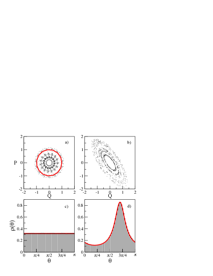
Figure 19: (Ref. [Mak-12, ], color online) a) phase space trajectory generated by Eq. (III.50) for H-array with $N=10^{4}$, $\varphi=\pi/15$, for zero disorder (solid circle), and for $\sigma^{2}=0.003$ (scattered points); b) one trajectory for M-array with $N=10^{6}$, $\varphi=2\pi/5$, $\sigma^{2}=0.003$. c) $\rho(\theta)$ from Eq. (III.50) for H-array (histogram), and Eq. (III.61) (horizontal line); d) $\rho(\theta)$ from Eq. (III.50) for M-array (histogram), and Eq. (III.62) (solid curve).

The principally different situation emerges for the M-array. In this case the Bloch phase (III.59) is identically zero. As a result, $W(\theta)=-U(\theta)U^{\prime}(\theta)$ in Eq. (III.7), and Eq. (III.7) leads to a highly nonuniform phase distribution

$$\rho(\theta)=\frac{1}{\pi}\sqrt{\varphi^{2}-\sin^{2}\varphi}\Big{/}U(\theta).$$ (III.62)

Fig. 19 displays perfect agreement between analytical expressions (III.61), (III.62) and data obtained by the iteration of the exact map (III.50).

To calculate the Lyapunov exponent via Eq. (III.56), one needs to perform an average with the distribution $\rho(\theta)$ given by Eq. (III.62). Surprisingly, usage of Eqs.  (III.56), (III.7) and (III.62) results in zero Lyapunov exponentTIM-FNT in the main (second order) approximation $\sim\sigma^{2}$. Therefore, the Lyapunov exponent is determined by next orders of the perturbation theory.

Unfortunately the direct evaluation of high order terms in $\rho(\theta)$ is rather cumbersome because of huge technical complexityTIM-FNT . The crucial step which enables authors of Ref. [Mak-12, ] to resolve the problem is the following. It is known that essential calculation difficulties are often related to the non-proper choice of dynamic variables. To understand how these variables should be chosen, let us analyze the numerical data displayed in Fig. 19. The b-panel in this figure demonstrates that the trajectory (i.e. the sequence of points $(Q_{n},P_{n})$ has the form of fluctuating ellipse specified by angle with respect to axes, and by fixed aspect ratio. This results in strongly non-uniform phase distribution (d-panel in Fig 19). Therefore, one should introduce new variables $\widetilde{Q}_{n}$, $\widetilde{P}_{n}$ by rotating and rescaling the axes $Q,P$, so that the trajectory transforms into fluctuating circle. Then, one can expect that the distribution of a new phase $\Theta_{n}$ in the considered approximation will be uniform.

To follow this recipe, let us rotate the vector $\vec{S}\to{\tilde{\vec{S}}}=\hat{R}\vec{S}$ with the help of unimodular matrix

$$\hat{R}=\left\|\begin{array}[]{ccc}\sqrt{\eta}\cos\tau&&\sqrt{\eta}\sin\tau\\ &&\\ -\displaystyle{\frac{\sin\tau}{\sqrt{\eta}}}&&\displaystyle{\frac{\cos\tau}{\sqrt{\eta}}}\end{array}\right\|,$$

where the angle $\tau$ describes rotation of the axes in $\vec{S}$-space, with further rescaling the axes due to free parameter $\eta$. In new coordinates the expressions (III.50) and (III.56) conserve their forms, however, with the rotated transfer matrix

$$\tilde{\hat{T}}=\hat{R}\hat{T}\hat{R}^{-1}.$$ (III.63)

$$\tilde{\vec{S}}_{n}=e^{\Xi_{n}}\left(\begin{array}[]{c}\cos\Theta_{n}\\ \\ \sin\Theta_{n}\end{array}\right).$$

Now the distribution $\rho(\Theta)$ for new phase $\Theta$ can be found starting from the quadratic expansion of Eq. (III.53) with new coefficients (III.63) and $\phi=0$,

$$\Theta_{n+1}-\Theta_{n} = [\eta_{\alpha}(n)-\eta_{\beta}(n)]V(\Theta_{n})+$$ (III.64)

$$\sigma^{2}V(\Theta_{n})V^{\prime}(\Theta_{n}).$$

Here the function $V(\Theta)$ is

$$V(\Theta)=\sin\varphi\sin(2\tau-\varphi)\sin 2\Theta$$

$$+\frac{\eta}{2}[\varphi-\sin\varphi\cos(2\tau-\varphi)][\cos 2\Theta-1]$$

$$-\frac{1}{2\eta}[\varphi+\sin\varphi\cos(2\tau-\varphi)][\cos 2\Theta+1].$$ (III.65)

The stationary Fokker-Plank equation corresponding to $\Theta$-map (III.64) reads

$$\frac{d}{d\Theta}\left[V^{2}(\Theta)\frac{d}{d\Theta}\rho(\Theta)+V(\Theta)V^{\prime}(\Theta)\rho(\Theta)\right]=0.$$

From this equation one gets that the phase distribution is uniform, $\rho(\Theta)=1/\pi$, and the trajectory is, indeed, a fluctuating circle provided that

$$\frac{d}{d\Theta}{V(\Theta)V^{\prime}(\Theta)}=0.$$ (III.66)

With the use of Eqs. (III.7) and (III.66), we now can obtain the desired expressions for the angle $\tau$, parameter $\eta$ and function $V(\Theta)$ (which is actually no more $\Theta$-dependent),

$$\tau=\frac{\varphi}{2},\ \ \ \eta^{2}=\frac{\varphi+\sin\varphi}{\varphi-\sin\varphi},$$

$$V(\Theta)=\sqrt{\varphi^{2}-\sin^{2}\varphi}.$$ (III.67)

The results presented in Fig. 20 confirm success of the chosen approach: in new variables the trajectory is a fluctuating circle and the phase distribution is uniform.

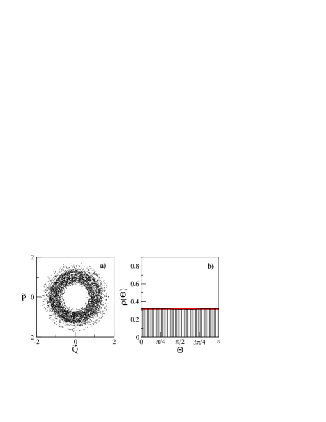
Figure 20: (Ref. [Mak-12, ], color online) (a) Phase space trajectory in new variables $(\widetilde{Q},\widetilde{P})$; (b) distribution $\rho(\Theta)$ generated by the transformed map with Eqs. (III.63) and (III.7), for $\gamma=0$, $\varphi=2\pi/5$, $\sigma^{2}=0.02$ and $N=10^{7}$.

The Lyapunov exponent $\gamma$ can be now obtained via Eq. (III.56) with the change $\theta_{n}\to\Theta_{n}$. Taking into account that $\gamma$ vanishes within quadratic approximation in disorder, we expand the $\Theta$-map of the form (III.53) with the coefficients (III.63) up to the fourth order in perturbation. By substituting the resulting expression into Eq. (III.56) and expanding the logarithm within the same approximation, after the averaging over $\Theta_{n}$ with uniform distribution, we arrive at final expression

$$\frac{1}{l_{\xi}}=\frac{\zeta\sigma^{4}}{4}\frac{[(2\varphi^{2}-\sin^{2}\varphi)\cos\varphi-\varphi\sin\varphi]^{2}}{\varphi^{2}-\sin^{2}\varphi}.$$ (III.68)

Here the constant

$$\zeta=\frac{\langle\delta(n)^{4}\rangle-\langle\delta(n)^{2}\rangle^{2}}{\langle\delta^{2}\rangle^{2}}$$

is specified by the form of distribution of $\delta_{\alpha,\beta}(n)$. For Gaussian and flat distributions we have $\zeta=0,-6/5$, respectively.

Equation (III.68) determines the asymptotics for large $\lambda\gg\max(\sigma,1)$,

$$\frac{1}{l_{\xi}}\equiv\gamma\approx\frac{2^{4}}{3^{3}5^{2}}(\zeta+2)\sigma^{4}k^{8},$$

that results in a quite surprising wavelength dependence of the localization length, $l_{\xi}\propto\lambda^{8}$. Thus, the dependence $l_{\xi}\propto\lambda^{6}$, numerically found for large $\lambda$ in Refs. Asatryan07 ; Asatryan10a and confirmed later in should be regarded as the intermediate one, apparently emerging due to not sufficiently large lengths $N$ over which the average of $\gamma$ is performed.

IV Localization in Complex Media

IV.1 Nonreciprocal Transmission in Magnetoactive Optical Structures

In this Subsection we present the results of analytical and numerical study of the Anderson localization of light propagating through random magnetoactive layered structures. We demonstrate that an interplay between strong localization and magnetooptical effects produces a number of non-reciprocity features in the transmission characteristics.

Magnetooptical effects and nonreciprocity are widely exploited in modern optics and applied physics Zvezdin ; Potton . In particular, magnetoactive periodic structures are currently attracting growing attention Lyubchanskii ; Inoue . The main phenomena of interest are the enhanced Faraday effect on resonances InoueAraiFujii and one-way propagation (nonreciprocal transmission) FigotinVitebsky ; YuWangFan ; Khanikaev ; KhanikaevSteel employed for the concept of optical insulators. The resonant Faraday effect has also been shown in connection with the localization of light in random layered structures InoueFujii .

Here we examine the transmission properties of one-dimensional random layered structures with magneto-optical materials. We employ short-wavelength approximation, where the localization is strong, and consider both Faraday and Voigt geometries. In the Faraday geometry, magneto-optical correction to the localization length $l$ results to a significant broadband non-reciprocity and polarization selectivity in the typical, exponentially small transmission. In the Voigt geometry, averaging over random phases suppresses the magneto-optical effect, in contrast to the case of periodic structures where it can be quite pronounced FigotinVitebsky ; KhanikaevSteel . At the same time, in both the geometries we reveal the nonreciprocal frequency shifts of narrow transmission resonances, corresponding to the excited localized states inside the structure Frisch ; BBF ; Bliokh-2 ; we-PRL-1 . This offers efficient unidirectional propagation at the given resonant frequency.

Consider the light transmission through the long stack composed with magnetooptical materials in the short-wavelength approximations. In the localized regime, we can neglect in Eq. (II.2) the external interface transfer matrices ${\hat{F}}^{0\alpha}$, ${\hat{F}}^{\beta 0}$ just replacing the exact matrix $\hat{T}$ by the truncated matrix $\hat{T}^{\prime}$

$$\hat{T}^{\prime}={\hat{F}}_{N}{\hat{S}}_{N}{\hat{F}}_{N-1}{\hat{S}}_{N-1}{\hat{F}}_{N-2}~{}...~{}{\hat{F}}_{2}{\hat{S}}_{2}{\hat{F}}_{1}{\hat{S}}_{1}.$$ (IV.1)

Then, if the wavelength within the $k$-th layer is much shorter than the variance of the layer thickness BerryKlein , then the phases $\varphi_{k}$ modulo $2\pi$ in the propagation matrices ${\hat{S}}_{j}$ (II.23) are independent and nearly uniformly distributed in the range $(0,2\pi)$. In this approximation, the transmittance corresponding to the transfer matrix (IV.1) after averaging over all phases $\varphi_{k}$, is reduced to the product of the transmittances of separate layers Baluni and, furthermore, to the product of transmittances of the interfaces only BerryKlein

$$\ln\left({\mathcal{T}}\right)\approx\sum_{j=1}^{2N}\ln\tau_{j}~{},~{}~{}\tau_{j}=1/|({\hat{F}}_{j})_{11}|^{2}.$$ (IV.2)

Substitution of Eq. (IV.2) into Eq. (II.1) in the limit $N\to\infty$ yields the simple expression for the localization length

$$\frac{1}{l}=\approx\frac{1}{2}{\ln\left|\left({\hat{F}}^{\alpha\beta}\right)_{11}\left({\hat{F}}^{\beta\alpha}\right)_{11}\right|}.$$ (IV.3)

in the short-wavelength approximation.

This result can be easily extended to any number of alternating layers. For instance, considering a random structure consisting of three types of alternating layers, ‘$\alpha$’, ‘$\beta$’, and ‘$\gamma$’, one has

$$\frac{1}{l}=\frac{1}{3}{\ln\left|\left({\hat{F}}^{\alpha\beta}\right)_{11}\left({\hat{F}}^{\beta\gamma}\right)_{11}\left({\hat{F}}^{\gamma\alpha}\right)_{11}\right|}.$$

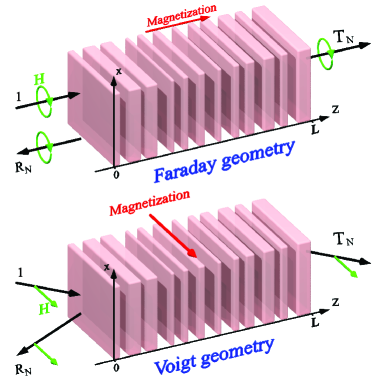
Figure 21: (Ref. [Bliokh-mag, ], color online.) Schematic picture of the wave transmission and reflection from a random-layered structure consisting of two types of alternating layers ‘$\alpha$’ (here – magnetoactive material) and ‘$\beta$’ (here – air) with random widths. Magnetization of the medium, wave polarizations and directions of propagation are shown for the Faraday and Voigt geometries.

Transmission through a one-dimensional lossless linear medium is always reciprocal if there is only one (but propagating in two directions) mode in the system. Indeed, while the forward transmission of the wave incident from the left on the medium is described by the $2\times 2$ transfer matrix ${\hat{T}}$ with transmission coefficient $T$ and transmittance ${\mathcal{T}}$, the backward transmission of the reciprocal wave incident from the right is characterized by the inverse transfer matrix ${\hat{T}}^{-1}$ with the same transmission coefficient and transmittanceBaluni ; BerryKlein .

If the system possesses two or more uncoupled modes labeled by index $\varsigma$, the waves are marked by the propagation direction $\upsilon$ and mode indices: $h^{\upsilon,\varsigma}$. Still, the forward and backward propagation of each mode $\varsigma$ through the system with incident waves of types $(+,\varsigma)$ and $(-,\varsigma)$ are described by the $2\times 2$ transfer matrices ${\hat{T}}^{\varsigma}$ and $({\hat{T}}^{\varsigma})^{-1}$ characterized by the same transmittance $\mathcal{T}^{\varsigma}$. However, the wave reciprocal to $(+,\varsigma)$ is determined by the time-reversal operation which changes $\upsilon\to-\upsilon$ (because of the $\mathbf{k}\to-\mathbf{k}$ transformation) but can also affect $\varsigma$ Potton . In particular, if the time reversal operation changes the sign of the mode index: $\varsigma\to-\varsigma$, then the reciprocal wave will be $(-,-\varsigma)$ rather than the backward wave of the same mode, $(-,\varsigma)$. Accordingly, the transmittances of the mutually reciprocal waves through the system, $\mathcal{T}^{\varsigma}$ and $\mathcal{T}^{-\varsigma}$, can be different. This signals nonreciprocity in the system.

Non-reciprocity in the system under consideration originates from the difference between the modes $\varsigma$ and $-\varsigma$, and does not depend explicitly on the direction of incidence $\upsilon$. Therefore, in practice, it is sufficient to compare only forward transmissions of the modes $\pm\varsigma$, described by the transfer matrices ${\hat{T}}^{\pm\varsigma}$ and transmittances $\mathcal{T}^{\pm\varsigma}$.

There are two main geometries typical for magneto-optical problems Zvezdin : the Faraday geometry, where the magnetization is collinear with the direction of propagation of the wave, and the Voigt (or Cotton-Mouton) geometry, where the magnetization is orthogonal to the direction of propagation of the wave (see Fig.21). Below we study the averaged transmission decrement and individual transmission resonances in both geometries and show that propagation of light in disordered magnetoactive layered media offers nonreciprocal transmission.

In the Faraday geometry both magnetization and the wave vector are directed across the layers, i.e., along the $z$-axis (see Fig.21). We assume that the magnetic tensor is equal to one and the magneto-optical effects are described exclusively by the dielectric tensor which in the Faraday geometry has the formZvezdin

$$\hat{\varepsilon}=\left\|\begin{array}[]{ccc}\varepsilon&-iQ&0\\ iQ&\varepsilon&0\\ 0&0&\varepsilon\\ &&\end{array}\right\|.$$

The eigenmodes of the problem are circularly polarized waves of magnetic $\mathbf{H}$

$$\mathbf{H}^{\upsilon,\varsigma}=\frac{H^{\upsilon,\varsigma}}{\sqrt{2}}\left(\begin{array}[]{c}1\\ i\varsigma\\ 0\\ \end{array}\right){\text{e}}^{i(\upsilon kz-\omega t)},\ \ \ \upsilon,\varsigma=\pm 1,$$ (IV.4)

and electric $\mathbf{E}$

$$\mathbf{E}^{\upsilon,\varsigma}=i\upsilon\varsigma\frac{k_{0}}{k}\mathbf{H}^{\upsilon,\varsigma}.$$ (IV.5)

fields. Here $H^{\upsilon,\varsigma}$ ($E^{\upsilon,\varsigma}$) are the wave amplitudes, whereas $k$ is the propagation constant affected by the magnetization parameter $q$ and depending on $\varsigma$.

$$k=nk_{0}\sqrt{1+\varsigma q},\ \ \ n=\sqrt{\varepsilon},$$

$$k_{0}=\frac{\omega}{c},\ \ \ \ \ \ q=\frac{Q}{\varepsilon}.$$ (IV.6)

In the linear approximation in $q$, $k\simeq nk_{0}(1+\varsigma q/2)$.

Parameter $\varsigma$ is the mode index which determines the direction of rotation of the wave field. In this manner, the product $\upsilon\varsigma$ represent the helicity

$$\chi=\upsilon\varsigma,$$

which distinguishes the right-handed ($\chi=+1$) and left-handed ($\chi=-1$) circular polarizations defined with respect to the direction of propagation of the wave. Note that the time reversal operation keeps helicity unchanged, whereas $\varsigma$ changes its sign Potton . Thus, the reciprocal wave is given by $\mathbf{H}^{-\upsilon,-\varsigma}$, precisely as described above.

The total field in a layer is the sum $\mathbf{H}^{+,\varsigma}+\mathbf{H}^{-,\varsigma}$ of the eigenvectors (IV.4) with the amplitudes $H^{\pm,\varsigma}.$ Consider the wave transformation at the interface between the media ‘$a$’ and ‘$b$’. The helicity of the wave flips upon the reflection and remains unchanged upon transmission. As a result, parameter $\varsigma$ remains unchanged, so that there is no coupling between the modes with $\varsigma=+1$ and $\varsigma=-1$ (see Fig.21), and these modes can be studied independently. From now on, for the sake of simplicity, we omit $\varsigma$ in superscripts and write explicitly only the values of the direction parameter $\upsilon=\pm 1$.

Using the standard boundary conditions for the wave electric and magnetic fields at the ‘$\alpha$’-‘$\beta$’ interface for the normalized fields

$$\vec{h}=\frac{k_{0}}{k}\left(\begin{array}[]{c}H^{+}\\ \\ H^{-}\end{array}\right),\ \ \ \ \ \ \ \ \vec{h}_{\alpha}={\hat{F}}^{\alpha\beta}\ \vec{h}_{\beta}$$

with the normalized interface transfer matrix

$${\hat{F}}^{\alpha\beta}=\frac{1}{2\sqrt{k_{\alpha}k_{\beta}}}\left\|\begin{array}[]{cc}\displaystyle{k_{\beta}+k_{\alpha}}&\displaystyle{k_{\beta}-k_{\alpha}}\\ \displaystyle{k_{\beta}-k_{\alpha}}&\displaystyle{k_{\beta}+k_{\alpha}}\\ &\end{array}\right\|,$$ (IV.8)

where $k_{\alpha,\beta}$ are the wave numbers (IV.1) in the corresponding media.

Calculating the localization decrement from Eq. (IV.3) with Eqs. (IV.1) and (IV.8), we obtain in the linear approximation in $q$:

$$\kappa=2\ln\frac{k_{\alpha}+k_{\beta}}{2\sqrt{k_{\alpha}k_{\beta}}}\simeq\kappa^{(0)}+\kappa^{(1)},$$

$$\kappa^{(0)}\!=\!\ln\frac{(n_{\alpha}+n_{\beta})^{2}}{4n_{\alpha}n_{\beta}},$$

$$\kappa^{(1)}\!=\!\frac{\sigma}{2}(q_{\alpha}-q_{\beta})\frac{n_{\alpha}-n_{\beta}}{n_{\alpha}+n_{\beta}}.$$ (IV.9)

Thus, the localization decrement acquires the first-order magneto-optical correction $\kappa^{(1)}$ caused by the Faraday effect. This correction depends on $\varsigma$, i.e., on the polarization helicity $\chi$ and the propagation direction $\upsilon$ through $\varsigma=\chi\upsilon$. For the reciprocal waves with the same $\chi$ and opposite $\upsilon$, $\kappa^{(1)}$ has opposite signs. This signals nonreciprocal localization in a Faraday random medium. In practice, the nonreciprocal difference in the transmission decrements (IV.1) can be observed by changing sign of either propagation direction $\upsilon$ (with the helicity fixed), or polarization $\chi$, or magnetization $q$.

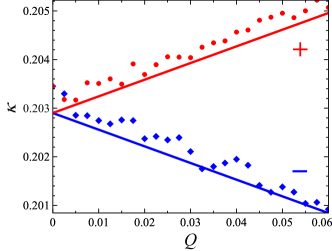
Figure 22: (Ref. [Bliokh-mag, ], color online) Localization decrement $\kappa$ vs. magneto-optical parameter $Q$ for opposite modes propagating through a two-component random structure in the Faraday geometry (see details in the text). The modes with $\varsigma=\pm 1$ correspond to either opposite circular polarizations or propagation directions. Numerical simulations of exact equations (symbols) and theoretical formula (IV.1) (lines).

Despite the magneto-optical correction to the localization decrement is small in magnitude, $\kappa^{(1)}\ll\kappa^{(0)}$, it still might result in a significant difference in the typical transmission spectrum. This difference is described by an additional factor of $\propto\exp[-2N\kappa^{(1)}]$ in transmittance, which is exponential with respect to the length of the structure. Hence, small correction (IV.1) brings about significant broadband nonreciprocity or polarization selectivity in the typical small transmission when $N\left|\kappa^{(1)}\right|\geq 1$.

Fig. 22 shows dependence of the localization decrement on the magnetization parameter $Q=\varepsilon q$ calculated numerically and compared to analytical result (IV.1). Numerical simulations were performed for the structure containing ${\mathcal{N}}=2N=90$ alternating layers of air ($\varepsilon=1,Q=0$), and bismuth iron garnet (BIG), with dielectric constant $\varepsilon=6.25$ and magneto-optic parameter reaching $Q=0.06$. The thicknesses of layers were randomly distributed in the range 50$\div$150 $\mu$m (i.e., $\bar{w}=100\mu$m, $d=50\mu$m), whereas the excitation wavelength was 632 nm. The averaging was performed over $10^{5}$ realizations of the random sample. One can see excellent agreement between numerical simulations and analytical results showing linear splitting of the $\varsigma=1$ and $\varsigma=-1$ localization decrements as a function of the magneto-optic parameter.

In the Voigt geometry, the dielectric tensor isZvezdin

$$\hat{\varepsilon}=\varepsilon\left\|\begin{array}[]{ccc}1&0&iq\\ 0&1&0\\ -iq&0&1\\ &&\end{array}\right\|.$$

The first-order interaction of the wave with the magnetization occurs only upon oblique propagation of the wave in the $xz$-plane, i.e., when $k_{x}=\text{const}\neq 0$ (see Fig.21).

The eigenmodes of the problem are the TE mode which is uncoupled from the magnetization, and TM mode with the tangential components

$$H_{y}^{\upsilon,\varsigma} = H^{\upsilon,\varsigma}\ \text{e}^{i(\varsigma xk_{\perp}+\upsilon zk_{\parallel}-\omega t)},$$

$$E_{x}^{\upsilon,\varsigma} = A^{\upsilon,\varsigma}H_{y}^{\upsilon,\varsigma}.$$

Here parameters $\upsilon=\pm 1$ and $\varsigma=\pm 1$ indicate propagation in the positive and negative $z$ and $x$ directions, respectively, $k_{\parallel}=\sqrt{k^{2}-k_{x}^{2}}$, $k_{\perp}=|k_{x}|$, whereas

$$A^{\upsilon,\varsigma} = -\left(A^{-\upsilon,\varsigma}\right)^{*}=\frac{i\varsigma qk_{\perp}+\upsilon k_{\parallel}}{\varepsilon(1-q^{2})k_{0}},$$ (IV.10)

$$k = nk_{0}\sqrt{1-q^{2}}.$$

In the linear approximation in $q$, $A^{\upsilon,\varsigma}\simeq(\upsilon k_{\parallel}+i\varsigma qk_{\perp})/(\varepsilon k_{0})$ and $k\simeq nk_{0}$ so that the magnetization affects imaginary parts (i.e., phases) of the amplitudes $A^{\upsilon,\varsigma}$ and does not affect the propagation constant, cf. Eqs. (IV.5) and (IV.1).

In the Voigt geometry, direction of the transverse wave vector component, $\varsigma$, serves as the mode index. The mutually reciprocal waves are $H^{\upsilon,\varsigma}$ and $H^{-\upsilon,-\varsigma}$ because the time reversal transformation reverts the whole wave vector, $\mathbf{k}\mapsto-\mathbf{k}$.

The parameter $\varsigma$ is not changed upon reflection and transmission through the layers, i.e., the modes with $\varsigma=\pm 1$ are uncoupled from each other. Therefore, for the sake of simplicity, we omit the mode index in superscripts, and write explicitly only the values of the direction parameter $\upsilon=\pm 1$.

Using the standard boundary conditions for the wave electric and magnetic fields at the ‘$\alpha$’-‘$\beta$’ interface, for the normalized interface transfer matrix ${\hat{F}}^{\alpha\beta}$ we obtainKhanikaevSteel

$${\hat{F}}^{\alpha\beta}=\frac{1}{\sqrt{4\mathrm{Re}A_{\alpha}^{+}\mathrm{Re}A_{\beta}^{+}}}\times$$

$$\left\|\begin{array}[]{cc}\displaystyle{A_{\beta}^{+}+A_{\alpha}^{+*}}&\displaystyle{A_{\alpha}^{+*}-A_{\beta}^{+*}}\\ \displaystyle{A_{\alpha}^{+}-A_{\beta}^{+}}&\displaystyle{A_{\alpha}^{+}+A_{\beta}^{+*}}\\ &\end{array}\right\|.$$

In contrast to the Faraday geometry, in the Voigt geometry the linear magneto-optical correction changes only phases of the transmission and reflection coefficients, whereas corrections to the interface transmittance start with the terms $\propto q^{2}$. In short-wave limit, only these transmittances determine the total transmittance, Eq. (IV.2). Therefore, a short-wavelength transmission through a random multilayered stack is reciprocal and is not affected by magnetization in the first-order approximation. In the short-wave limit, this statement remains true for any number of types of alternating layers. It was verified numerically for the three-layer systemBliokh-mag . At the same time, a periodic structure with a cell consisting of three different layers (which breaks the mirror reflection symmetry) can demonstrate significant nonreciprocity YuWangFan ; KhanikaevSteel but beyond the short-wave approximation.

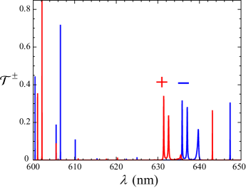
Figure 23: (Ref. [Bliokh-mag, ], color online.) Transmission spectra of a random magneto-optical sample in the Faraday geometry (see details in the text) for waves with $\varsigma=\pm 1$. While the averaged localization decrements are only slightly different (Fig.22), all individual resonances are shifted significantly as compared with their widths, Eq. (IV.12).

Averaged localization decrement is associated with exponential decay of the incident wave deep into the infinite sample Baluni ; Ping91 ; FG ; BerryKlein . For a finite sample, this is so only for typical realizations. However, there exist some resonant realizations of the sample at a given frequency (or, equivalently, resonant frequencies for a given realization) where transmission is anomalously high and is accompanied by the accumulation of energy inside the sample. Lifshits ; Frisch ; BBF Such resonant transmission corresponds to excitation of the Anderson localized states (quasi-modes) inside the sample. Akin to the resonant localized states in photonic crystal cavities, the transmission resonances in random structures are extremely sensitive to small perturbations: realizationLifshits , absorption,BBF nonlinearity, Shadrivov and, as we show here, magnetoactivity.

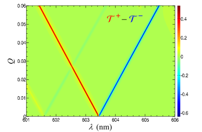
Figure 24: (Ref. [Bliokh-mag, ], color online.) Differential transmittance, ${\mathcal{T}}^{+}-{\mathcal{T}}^{-}$, for two resonances from Fig.22 as dependent on the value of magneto-optical parameter $Q$, cf. Eq. (IV.12).

Figure 23 shows transmission spectra for two modes $\varsigma=\pm 1$ (i.e., either with opposite helicities or propagation directions) in one realization of a magnetooptical sample in the Faraday geometry. The parameters of the sample are the same as in Section IIIA with $Q=0.06$. One can see strong splitting of the $\varsigma=\pm 1$ transmission resonances which have exponentially narrow widthsBBF $\propto\kappa\exp(-\kappa N)/2\bar{w}$ . This offers strongly nonreciprocal, practically unidirectional, propagation or polarization selectivity in the vicinity of resonant frequencies.

To estimate the splitting of resonances, we note that the wavenumbers in magnetooptical materials are shifted due to the Faraday effect, Eq. (IV.1). Hence, the shifts of the resonant wavenumbers of the random Faraday medium can be estimated by averaging of this shift over different materials in the structure:

$$\Delta k_{\mathrm{res}}\simeq\varsigma\,\overline{\frac{qnk_{0}}{2}},$$ (IV.12)

where $\overline{(...)}$ stands for some average of $(...)$. Using $\overline{qn}\sim(q_{a}n_{a}+q_{b}n_{b})/2$ for estimation in the two-component structure, we obtain $\Delta\lambda_{\mathrm{res}}\sim-\varsigma\,3.6$ nm, which agrees with the $\varsigma$-dependent splitting observed in Fig. 23.

Figure 24 displays the differential transmission for the waves with $\varsigma=+1$ and $\varsigma$ lying in a narrow frequency range in Fig. 23. In agreement with estimation (IV.12), one observes the linear dependence of the resonance splitting on magnetization.

In the Voigt geometry, the resonances also allow nonreciprocal transmission and demonstrate splitting of the resonant frequencies. In Fig. 25, the differential transmission is shown for reciprocal waves with $\varsigma=\pm 1$ in the vicinity of one resonance for the three-component structure considered in Section IIIB. The splitting is very small in this case, and $\varsigma=+1$ and $\varsigma=-1$ resonances overlap significantly. Because of this, the differential transmittance in Fig. 25 is tiny, its amplitude linearly grows with $Q$, whereas the frequency positions of its maximum and minimum correspond to the width of the original resonance and are practically unchanged.

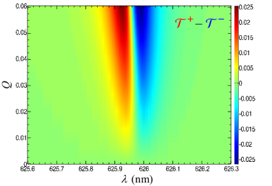
Figure 25: (Ref. [Bliokh-mag, ], color online.) Differential transmittance, ${\mathcal{T}}^{+}-{\mathcal{T}}^{-}$, for in the vicinity of a single resonance in the Voigt geometry (see Section IIIB for details) as dependent on the magneto-optical parameter $Q$.

Unlike the wave-number shift in the Faraday geometry, the nonreciprocal shift of resonant frequencies in the Voight geometry arises from the phases of the amplitudes $A$, Eq. (IV.10). These phases are responsible for the phases of transmission coefficients between the layers and can be estimated as $\phi\sim q(\varsigma k_{\perp})/(\upsilon k_{\parallel})\equiv q\tan\theta$, where $\theta$ is the angle of propagation with respect to the $z$-axis. The phases accumulated at a layer effectively shift the wave numbers as $\upsilon\Delta k_{\parallel}=\Delta k\cos\theta\sim\phi/w$, where $w$ is the thickness of the layer. Averaging over different materials in the random layered structure, we estimate the nonreciprocal shift of the resonant wave number:

$$\Delta k_{\mathrm{res}}\sim\overline{\frac{q\sin\theta}{w\cos^{2}\theta}}=\varsigma\,\overline{\frac{q|\sin\theta|}{w\cos^{2}\theta}}.$$

This shift is $\varsigma$-dependent, i.e., nonreciprocal, and much smaller than the Faraday-geometry shift (IV.12) as $k\bar{w}>kd\gg 2\pi$ in the short-wavelength limit. For the parameters in use, with $Q=0.06$, we have $\Delta\lambda_{\mathrm{res}}\sim-\varsigma\,3\cdot 10^{-4}$nm, which agrees with the data plotted in Fig. 25.

IV.2 Charge Transport in Disordered Graphene

Shortly after the discovery of highly unusual physical properties of graphene it was realized that the electron transport in this material had many common features with the propagation of light in dielectrics. Historically, the analogy between Maxwell equations and those used in the relativistic electron theory has been discussed in different contexts and for various purposes (see, for example, BiBi ; Zalesny ; BFSN ; Mehrafarin ) since 1907 when Maxwell equations were reduced Silberstein to an alternative, more concise form by introducing a complex field $\mathbf{F}=\mathbf{E}+i\mathbf{H}$:

$$c\hat{\boldsymbol{\rho}}\cdot\nabla\Psi=-n\partial\Psi/\partial t,$$ (IV.13)

where $\Psi$ is the 4-vector with components $-F_{x}+iF_{y}$, $F_{z}$, $F_{z}$, $F_{x}+iF_{y}$, $n$ is the refraction index, and the components of the 3-vector $\hat{\boldsymbol{\rho}},$ are the Dirac matrices $\hat{\rho_{i}},$ $i=1,2,3$ (Pauli matrices in which the units are replaced by the unit $2\times 2$ matrices).

In the last few yeas, this activity perked up due to the recent developments in the physics of graphene. Nowadays it is well understood that under some (rather general) conditions, Dirac equations describing the charge transport in a graphene superlattice created by applying inhomogeneous external electric potential could be reduced to Maxwell equations for the propagation of light in a dielectric medium. To better understand the physics of charge transport in graphene subject to a coordinate-dependent potential, in what follows, we compare the results for graphene with those for the propagation of light in layered dielectric media (for more analogies between quantum and optical systems, see, e.g. Ref.Dragoman ; analogy ). Additional analogies, not discussed here, also exist with the transport and localization of phonons in different kinds of periodic and random one-dimensional structures Nori ; Nori_1 ; Nori_2 .

As it was shown above, the light transport of electromagnetic waves in multilayered media is described in terms of the transfer matrices of two types. The first type is formed by diagonal matrices $\hat{S}_{j}$ corresponding to the propagation of wave through the $j$-th layer. These matrices are the same as in Eq. (II.23) (up to the signs of the exponent). The second type is formed by the interface transfer matrices $\hat{F}_{j,j+1}$ describing transformation of the amplitudes of the electromagnetic waves at the interface between $j-$th and $(j+1)-$th layers and having the form

$$\hat{F}_{j,j+1}={\frac{1}{2\cos\theta_{j+1}}}\left\|\begin{array}[]{cc}G_{j,j+1}^{(+)}&G_{j,j+1}^{(-)}\\ G_{j,j+1}^{(-)}&G_{j,j+1}^{(+)}\end{array}\right\|,$$ (IV.14)

where

$$G_{j,j+1}^{(\pm)}=\cos\theta_{j+1}\pm\cos\theta_{j}\cdot\mathrm{sgn}(\nu_{j}\nu_{j+1}){\frac{Z_{j+1}}{Z_{j}}}$$ (IV.15)

for $s$-polarized waves and

$$G_{j,j+1}^{(\pm)}={\frac{Z_{j+1}}{Z_{j}}}\cos\theta_{j+1}\pm\cos\theta_{j}\cdot\mathrm{sgn}(\nu_{j}\nu_{j+1})$$ (IV.16)

for $p$-polarized waves. Here, $\theta_{j}$ is the angle of the propagation within the $j-$th layer, $Z_{j}$ and $\nu_{j}$ are the impedance and the refractive index of the $j$th layer defined by Eq. (III.1). Signs $\pm$ correspond, respectively, to $R-$ and $L-$ dielectric layers with positive and negative refractive indices.

In the case of the charge transport in a graphene superlattice created by a piecewise-constant electrostatic potential depending on one coordinate $x$ in the plane $(x,y)$ of the graphene layer, the analogues transfer matrix, which describes the transition through the interface between adjacent regions with different values of the potential, has the form BFSN

$$\hat{\mathcal{F}}_{j,j+1}={\frac{1}{2\cos\theta_{j+1}}}\left\|\begin{array}[]{cc}\mathcal{G}_{j,j+1}^{(+)}&\mathcal{G}_{j,j+1}^{(-)}\\ (\mathcal{G}_{j,j+1}^{(-)})^{\ast}&(\mathcal{G}_{j,j+1}^{(+)})^{\ast}\end{array}\right\|,$$ (IV.17)

where

$$\mathcal{G}_{j,j+1}^{(\pm)}=e^{-i\theta_{j+1}}\pm e^{\pm i\theta_{j}}\cdot\mathrm{sgn}[(\varepsilon-u_{j})(\varepsilon-u_{j+1})],$$ (IV.18)

Here the $\theta_{j}$ is given by equation $\tan\theta_{j}=\beta/\sqrt{(\varepsilon-u_{j})^{2}-\beta^{2}}$ where $\beta$ is the projection of the dimensionless momentum on $y$ axis, $\varepsilon$ and $u_{j}$ are the dimensionless energy of the charge carrier and the scalar potential of the $j$-th layer. If $\theta_{j}$ is real, it coincides with the angle of the propagation of electron within the $j$-th layer.

Comparison of Eqs. (IV.14) and (IV.17) shows that the role of the refractive index $\nu$ in graphene is played by the difference $\varepsilon-u$. In particular, a layer, in which the potential exceeds the energy of the particle, $u>\varepsilon$, is similar to a $L$-slab with negative refractive index (metamaterial), while a layer where $u<\varepsilon$, is similar to normal material. It is due to this similarity that a junction of two regions having opposite signs of $u-\varepsilon$ (so-called p-n junction) focuses Dirac electrons in grapheneCheianov , in the same way as an interface between left- and right-handed dielectrics focuses electromagnetic wavesVeselago .

This analogy is not complete: although the equations are akin, the boundary conditions are, generally speaking, different. As a result Eq. (IV.18) (for graphene) does not contain factor $Z_{j+1}/Z_{j}$ which is present in Eqs. (IV.15), (IV.16) and determines the reflection coefficients at the boundary between two dielectrics born wolf . Another important distinction between transfer matrices $\hat{\mathcal{F}}$ (graphene) and $\hat{F}$ (electromagnetic waves) is that $\hat{\mathcal{F}}$ is a complex-valued matrix, while the $\hat{F}$ is always real. This is manifestation of the fundamental difference between graphene wave functions and electromagnetic fields in dielectrics. The graphene wave functions are complex-valued spinors which describe two different physical objects: particles (electrons) and antiparticles (holes). The electromagnetic fields are real that reflects the fact that photons do not have antiparticles (antiphoton is identical with photon). These distinctions bring about rather peculiar dissimilarities between the conductivity of graphene and the transparency of dielectrics.

However in the particular case of normal incidence $\theta_{j}=\theta_{j+1}=0$ and equal impedances $Z_{j}=Z_{j+1}$, the transmission of Dirac electrons through a junction is similar to the transmission of light via an interface between two media with different refractive indices (but equal impedances). Such an interface is absolutely transparent to light and therefore both p-n and p-p junctions are absolutely transparent to the Dirac electrons in grapheneCheianov ; Katsnelson1 . This is related to the absence of backscattering and antilocalization of massless Dirac fermions caused by their spin properties anti1 ; anti2 . This also explains Klein paradoxKlein (perfect transmission through a high potential barrier) in graphene systems, and leads (together with symmetry and spectral flow arguments) to the surprising conclusion that Dirac electrons are delocalized in disordered 1D graphene structure, providing a minimal non-zero overall transmission, which cannot be destroyed by fluctuations, no matter how strong they are Titov-1 . However, this statement (being correct in some sense) should be perceived with a certain caution. Indeed, many features of Anderson localization can be found in random graphene systems. It has been shown in Mehrafarin that although the wave functions of normally incident ($\theta=0$) particles are extended and belong to the continuous part of the spectrum, away from some vicinity of $\theta=0,$ 1-D random graphene systems manifest all features of disorder-induced strong localization. In particular, for a long enough, disordered graphene superlattice the transmission coefficient, $T$, as a function of the angle of incidence, $\theta$, (or of the energy $E$, if $\theta\neq 0$ is fixed) has typical for Anderson localization shape, Fig. 26.

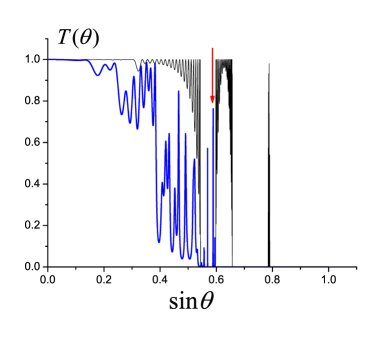
Figure 26: (Ref. [BFSN, ]) Transmission coefficient $T(\theta)$ for periodic (thin black line) and disordered (bold blue line) graphene.

Along with continuous of typical angles (or energies), for which the transmission is exponentially small, there exists a quasi-discrete random set of directions where the sample is well transparent, i.e., the transmission coefficient is close to one. At these angles, the wave functions are exponentially localized (Fig. 27), with the Lyapunov exponent (inverse localization length $l_{\xi}$) being proportional to the strength of disorder.

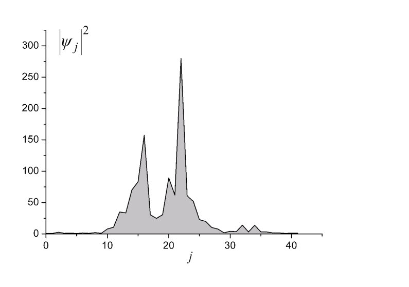
Figure 27: (Ref. [BFSN, ]) Spatial distribution of the wave function localized inside the sample for $\theta$ marked by red arrow in Fig. 26

Charge transport in a graphene sheet subjected to a disordered electrostatic potential is determined by the ratio between its values $u(\xi)$ and the energy $\varepsilon$ of the particle. In particular, in randomly-layered potential $u_{j}=u_{0}(j)+\Delta u_{j}$ ($j$ is the number of a layer, $u_{0}(j)$ is a non-random function, $\Delta u_{j}$ are independent random variables homogeneously distributed in the interval $[-\delta u,\delta u]$) it manifests essentially different features in the following three different systems Mehrafarin :

(i) $u_{j}<\varepsilon$, $u_{0}(j)$ is a periodic function. In this case, a relatively weak disorder drastically changes the transmission spectrum. All features of the spectrum of the underlying periodic structure are washed out, and a rather dense (quasi-)discrete angular spectrum appears, with the corresponding wave functions being localized at random points inside the sample (disorder-induced resonances). However, there is one fundamental difference from the usual Anderson localization: in the vicinity of normal incidence, the transmission spectrum of graphene is continuous with extended wave functions, and the transmission coefficient is finite ($T=1$ at $\theta=0)$. It is this range of angles that provides the finite minimal conductivity, which is proportional to the integral of $T(\theta)$ over all angles $\theta$.

(ii) $\varepsilon\leq u_{0}(j)=\mathrm{const.}$Under these conditions, the transmission of the unperturbed system is exponentially small (tunneling) and, rather unusually, gets enhanced by the fluctuation of the potential.

(iii) $\varepsilon=0$, $u_{0}(j)$ is a periodic set of numbers with alternating signs. The behavior of the charge carriers in the potential of this type is most unusual. It is characteristic of two-dimensional Fermions and have no analogies in electron and light transport. The disorder obliterates the transmission peaks of the underlying periodic system, makes much wider the transparency zone around normal angle of incidence, and gives rise to a new narrow peak in the transmission coefficient, associated with wave localization in the random potential. Unlike the peaks in the periodic structure, the wave function of this disorder-induced resonance is exponentially localized. In distinction to the case (i), the transmission in (iii) is extremely sensitive to fluctuations of the applied potential: relative fluctuations $\Delta u/u_{0}=0.05$ reduce the angular width of the transmission spectrum more than four times.

Propagation of light in analogous L-R and R-R disordered dielectric structures demonstrates completely different behavior. As the degree of disorder (variations of the refractive index) grows, the averaged angular spectra quickly reach their asymptotic “rectangular” shape: a constant transmission in the region where all interfaces between layers are transparent followed by an abrupt decrease in transmission in the region of angles where the total internal reflection appears.

IV.3 Bistability of Anderson Localized States in Nonlinear Media

Recent renewed interest to Anderson localization is driven by a series of experimental demonstrations in optics optics ; Segev ; Silberberg and Bose-Einstein condensates BEC ; BEC1 . One of the important issues risen in these studies is that the disordered systems can be inherently nonlinear, so that an intriguing interplay of nonlinearity and disorder could be studied experimentally.

Nonlinear interaction between the propagating waves and disorder can significantly change the interference effects, thus fundamentally affecting localization nonlin-loc1 ; nonlin-loc2 ; Soven ; Azbel . However, most of the studies of the localization in random nonlinear media deal with the ensemble-averaged characteristics of the field, such as the mean field and intensity, correlation functions, etc. These quantities describe the averaged, typical behavior of the field, but they do not contain information about individual localized modes (resonances), which exist in the localized regime in each realization of the random sample Soven ; Azbel ; BBF ; we-PRL-1 ; Topolancik . These modes are randomly located in both real space and frequency domain and are associated with the exponential concentration of energy and resonant tunneling. In contrast to regular resonant cavities, the Anderson modes occur in a statistically-homogeneous media because of the interference of the multiply scattered random fields. Although the disorder-induced resonances in linear random samples have been the subject of studies for decades, the resonance properties of nonlinear disordered media have not been explored so far.

In this Section we present the study of the effect of nonlinearity on the Anderson localized states in a one-dimensional random medium Shadrivov . As a result of interplay of nonlinearity and disorder, the bistability and nonreciprocity appear upon resonant wave tunneling and excitation of disorder-induced localized modes in a manner similar to that for regular cavity modes. At the same time, weak nonlinearity has practically no effect on the averaged localization background.

First, let us consider a stationary problem of the transmission of a monochromatic wave through a one-dimensional random medium with Kerr nonlinearity. The problem is described by the equation

$$\frac{d^{2}\psi}{dx^{2}}+k^{2}\left[n^{2}-\chi|\psi|^{2}\right]\psi=0~{},$$ (IV.19)

where $\psi$ is wave field, $x$ is coordinate, $k$ is wave number in the vacuum, $n=n(x)$ is the refractive index of the medium, and $\chi$ is the Kerr coefficient.

In the linear regime, $\chi|\psi|^{2}=0$, the multiple scattering of the wave on the random inhomogeneity $n^{2}(x)$ brings about Anderson localization. The main signature of the localization is an exponential decay of the wave intensity, $I=|\psi|^{2}$, deep into the sample and, thus, an exponentially small transmission And ; LGP ; Ping91 ; BerryKlein : $I_{\mathrm{out}}^{\mathrm{(typ)}}\sim I_{\mathrm{in}}\exp(-2L/l)\ll 1$. Here $L$ is the length of the sample and $l$ is the localization length which is the only spatial scale of Anderson localization. Along with the typical wave transmission, there is an anomalous, resonant transmission, which accompanies excitation of the Anderson localized states inside the sample and occurs at random resonant wave numbers $k=k_{\mathrm{res}0}$ Soven ; Azbel ; BBF ; we-PRL-1 ; Topolancik . In this case, the intensity distribution in the sample is characterized by an exponentially localized high-intensity peak inside the sample, $I_{\mathrm{peak}}\gg I_{\mathrm{in}}$, and a transmittance much higher than the typical one: $I_{\mathrm{out}}^{\mathrm{(res)}}\gg I_{\mathrm{out}}^{\mathrm{(typ)}}$.

Excitation of each localized mode inside the random sample can be associated with an effective resonator cavity located in the area of field localization and bounded by two potential barriers with exponentially small transparencies Bliokh-2 . According to this model, the transmittance spectrum $T(k,I_{out})$ in the vicinity of a resonant wavelength for the case of weak nonlinearity ($\chi|\psi|^{2}\ll 1$) is given in the form BBF ; Genack1 ; Shadrivov :

$$T(k,I_{\mathrm{out}})\equiv\frac{I_{\mathrm{out}}}{I_{\mathrm{in}}}=\frac{T_{\mathrm{res}}}{1+\left[A\chi I_{\mathrm{out}}+\delta\right]^{2}}~{},$$ (IV.20)

where $T_{res}$ is the transmission coefficient at resonance, and dimensionless parameters $A$ and $\delta$ characterize, respectively, the strength of the nonlinear feedback and the detuning from the resonant wave number:

$$A=\frac{2Q}{\chi}\left.\frac{d\ln k_{\mathrm{res}}}{dI_{\mathrm{out}}}\right|_{I_{\mathrm{out}}=0},~{}\delta=2Q\left(1-\frac{k}{k_{\mathrm{res}0}}\right).$$ (IV.21)

Equation ( IV.20) establishes relation between the input and output wave intensities, which is given by a cubic equation with respect to $I_{\mathrm{out}}$. It has a universal form typical for nonlinear resonators possessing optical bistability Bistability . From Eq. (IV.21) it follows that in the region of parameters:

$$A\delta<0~{},~{}~{}\delta^{2}>3~{},~{}~{}|\chi|I_{\mathrm{in}}>\frac{8}{3\sqrt{3}}\frac{1}{|A|T_{\mathrm{res}}}~{},$$

the dependence $I_{\mathrm{out}}(I_{\mathrm{in}})$ is of the S-type and the stationary transmission spectrum $T(k)$ is a three-valued function. In most cases, one of the solutions is unstable, whereas the other two form a hysteresis loop in the $I_{\mathrm{out}}(I_{\mathrm{in}})$ dependence (see Figs. 28 and 29).

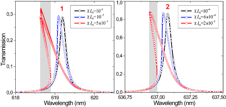
Figure 28: (Ref. [Shadrivov, ], color online.) Nonlinear deformations of the transmission spectra of two random resonances at different intensities of the incident wave. Numerical simulations of the Eq. IV.19 (curves) and theoretical Eq. IV.20 (symbols) are shown for the case of defocusing nonlinearity, $\chi>0$. Light-grey stripes indicate three-valued regions for the high-intensity curves, where only two of them (corresponding to the lower and upper branches) are stable.

It is important to emphasize two features of the equations (IV.20) and (IV.21), describing the nonlinear resonant transmission through a localized state. First, they have been derived without any approximations apart from the natural smallness of the nonlinearity and Lorentzian shape of the spectral line. Second, although the resonant transmission, the effect of nonlinearity, and bistability owe their origin to the excitation of the Anderson localized mode inside the sample, equations (IV.20) and (IV.21) contain only quantities which can be found via outside measurements Shadrivov .

Figure 28 shows nonlinear deformations of the resonant transmission spectra $T(k)$ for different values of $I_{\mathrm{in}}$, which exhibit transitions to bistability. The analytical dependence $T(k)$ given by Eqs. (IV.20, IV.21) with the parameters $T_{\mathrm{res}}$, $Q$, and $A$ found from the numerical experiments are in excellent agreement with the direct numerical solutions of Eq. (IV.19) remark . In numerical simulations of stationary regime we used the standard 4-th order Runge-Kutta method. We note, that the incident field amplitude is a single-valued function of the transmitted field. Thus, we solve second-order ordinary differential equation Eq. (IV.19) using transmitted field value as the boundary conditions for the equation.

The dimensionless parameters $T_{\mathrm{res}}$, and $Q$ from Eqs. (IV.20, IV.21), can also be estimated from a simple resonator model of the Anderson localized states BBF ; we-PRL-1 ; Bliokh-2 :

$$T_{\mathrm{res}}=\frac{4T_{1}T_{2}}{\left(T_{1}+T_{2}\right)^{2}}~{},~{}~{}Q^{-1}\sim\frac{T_{1}+T_{2}}{4k_{\mathrm{res}0}l}~{},$$ (IV.22)

where

$$T_{1}\sim\exp\left[-2x_{\mathrm{res}}/l\right]~{},~{}~{}T_{2}\sim\exp\left[-2(L-x_{\mathrm{res}})/l\right]~{}$$

are the transmission coefficients of the two barriers that form the effective resonator, $x_{\mathrm{res}}$ is the coordinate of the center of the area of field localization, $l$ is the localization length, and $L$ is the length of the sample.

Introducing a weak Kerr nonlinearity into the resonator model, one can also estimate the nonlinear feedback parameter $A$:

$$A\sim Q/\overline{n^{2}}T_{2}~{},$$ (IV.23)

where $\overline{n^{2}}$ is the mean value of $n^{2}(x)$.

It is important to note that each disorder-induced resonance is associated with its own effective cavity, so that the disordered sample can be considered as a chain of randomly located coupled resonators Ref-exp-2 .

Equations (IV.22, IV.23) enable one to estimate the values of the parameters describing the nonlinear resonant wave tunneling in Eqs. (IV.22, IV.23) by knowing only the basic parameters of the localization – the localization coordinate and the localization length. In particular, substituting Eqs. (IV.22, IV.23) into Eq. (IV.21) and taking into account that the most pronounced transmission peaks correspond to the localized states with $x\simeq L/2$ and $T_{1}\sim T_{2}$, we estimate the incident power needed for bistability of localized states

$$|\chi|I_{\mathrm{in}}\gtrsim\frac{\exp(-2L/l)}{k_{\mathrm{res}0}l}~{}.$$ (IV.24)

For the parameters used in our simulations this gives quite reasonable value $|\chi|I_{\mathrm{in}}\gtrsim 10^{-5}$. If we increase the length of the sample, the Q-factors of the resonances grow, and the incident power needed to observe the bistability becomes smaller.

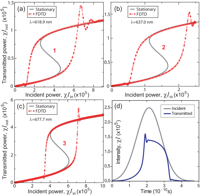
Figure 29: (Ref. [Shadrivov, ], color online.) Stationary and FDTD simulations showing hysteresis loops in the output vs. input power dependence for three different resonances. Panel (d) shows deformation of the transmitted Gaussian pulse corresponding to the hysteresis switching on the resonance 2.

To demonstrate temporal dynamics upon the bistable resonant tunneling, an explicit iterative nonlinear finite-difference time-domain (FDTD) scheme was implemented. For precise modeling of the spectra of narrow high-Q resonances, fourth-order accurate algorithm was used, both in space and in time fourthorder , as well as the Mur boundary conditions to simulate open boundaries and total-field/scattered-field technique for exciting the incident wave. Sufficient accuracy was achieved by creating a dense spatial mesh of 300 points per wavelength ($dx=\lambda/300$). To assure stability of the method in nonlinear regime, the time step was selected as $dt=dx/3c$, and each simulation ran for $N=2*10^{8}$ time steps. To compare the results of the FDTD simulations with the steady-state theory, the transmission of long Gaussian pulses with central frequencies and amplitudes satisfying conditions (IV.24) was considered, see Fig. 29(d). With an appropriate choice of the signal frequencies, we observe hysteresis loops in the $I_{\mathrm{out}}(I_{\mathrm{in}})$ dependencies which are in excellent agreement with stationary calculations, as shown in Figs. 29(a–c). Characteristic transitional oscillations accompany jumps between two stable branches, and strong reshaping of the transmitted pulse evidences switching between the two regimes of transmission, Fig. 29(d). We note, that different choice of the signal frequencies near the resonance can lead to various other behaviors of output vs. input curves, with transmission either increasing, when nonlinear resonance frequency shifts towards the signal frequency, or decreasing in the opposite case.

In addition to the bistability, the resonant wave tunneling through a nonlinear disordered structure is nonreciprocical. As is known for regular systems, nonsymmetric nonlinear systems may possess nonreciprocal transmission properties, resembling the operation of a diode. An all-optical diode is a device that allows unidirectional propagation of a signal at a given wavelength, which may become useful for many applications diode . A disordered structure is naturally asymmetric in the generic case, and one may expect a nonreciprocal resonant transmission in the nonlinear case. To demonstrate this, we modeled propagation of an electromagnetic pulse impinging the same sample from different sides and monitor the transmission characteristics. One case of such nonreciprocical resonant transmission is shown in the panel (a) of Fig.30. We observe considerably different transmission properties in opposite directions with the maximal intensity contrast between two directions 7.5:1. Moreover, the threshold of the bistability is also significantly different for two directions: there is a range of incident powers, for which the wave incident from one side of the sample is bistable, while there is no signs of bistability for the incidence from the other side. Figure 30(b) shows the pulse reshaping for incidence from opposite sides of the structure.

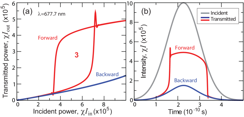
Figure 30: (Ref. [Shadrivov, ], color online) (a) Non-reciprocal transmission through the nonlinear disordered structure, showing different output powers for identical waves incident from different directions. (b) Corresponding shape of the incident pulse, and pulses transmitted in different directions.

In this Section we have presented the study of new manifestations of the interplay between nonlinearity and disorder. It is shown that even weak nonlinearity affect dramatically the resonant transmission associated with the excitation of the Anderson localized states leading to bistability and nonreciprocity. Despite random character of the appearance of Anderson modes, their behavior and evolution are rather deterministic, and, therefore, these modes can be used for efficient control of light similar to regular cavity modes. These results demonstrate that, unlike infinite systems, the Anderson localization in finite samples is not destroyed by weak nonlinearity – instead it exhibits new intriguing features typical for resonant nonlinear systems.

V Conclusions

We have reviewed the transmission and localization wave properties of the complex disordered structures composed of (i) left-handed metamaterials, (ii) magneto-active optical materials, (iii) graphene superlattices, and (iv) nonlinear dielectric media. Interference origin of the wave localization, together with strong energy concentration, makes Anderson localization highly sensitive to weak modifications of the material properties. We have shown that the exotic properties of novel materials can drastically modify the main features of the wave localization. This brings about anomalous pronounced dependences of the wave transmittance and localization length on both wave and material parameters: frequency, angle of incidence, polarization, magnetization, nonlinearity, etc. As a result, remarkable phenomena appear, such as anti-(de-)localization, unidirectional transmission, slow-light propagation, and bistability.

We have described a number of novel features accompanying the wave localization in complex media, including: (i) dramatic suppression of localization in mixed stacks with left-handed metamaterials, (ii) Brewster, zero-$\varepsilon$, and zero-$\mu$ delocalization, and (iii) anomalous transmission enhancement in periodic metamaterials with only one disordered electromagnetic characteristics, (iv) nonreciprocal localization and unidirectional transmission through magneto-active disordered stacks, (v) angle-dependent transmission resonances in graphene superlattices, and (vi) bistability and nonreciprocity of transmission resonances in nonlinear disordered structures.

We believe that presented results significantly extend and enrich theory and potential application of the wave localization in complex disordered media. In particular, they provide a theoretical toolbox which can serve for design of novel optical and electronic devices with unusual transport properties.

VI Acknowledgments

We are pleased to dedicate this review paper to 80-th anniversary of Academician Victor Valentinovich Eremenko and wish him a good health, good mood, and new scientific achievements.

We also thank our co-authors especially L.C. Botten, M.A. Byrne, R.C. McPhedran, F. Nori, P. Rajan, and S. Savel’ev, for fruitful collaboration and discussions of many original results summarized in this review paper. S.G. is grateful to N.M. Makarov, P. Markos, and L.A. Pastur for useful comments and helpful discussions.

This work was partially supported by the European Commission (Marie Curie Action). V.F acknowledges partial support from the Israeli Science Foundation (Grant # 894/10)

References

- (1) P. W. Anderson, Phys. Rev. 109, 1492 (1958).
- (2) I. M. Lifshits, S. A. Gredeskul, and L. A. Pastur, Vvedenye v Teoriu Neuporyadochennykh System (Nauka, Moskva 1987); Introduction to the Theory of Disordered Systems (Wiley, New York 1987).
- (3) Y. Imry. Introduction to Mesoscopic Physics (Oxford University Press, Oxford 2002).
- (4) S. John, Phys. Rev. Lett., 53, 2169 (1984).
- (5) P. Sheng, Scattering and localization of classical waves in random media (Singapore: World Scientific 1991).
- (6) P. Sheng, Introduction to Wave Scattering, Localization, and Mesoscopic Phenomena (Academic, San Diego, 2007).
- (7) P. Marcos, C.M. Soukoulis, Wave Propagation from Electrons to Photonic crystals and Left-handed materials, (Princeton University Press, Princeton, 2008).
- (8) E. Abrahams (Ed.), 50 Years of Anderson Localization, World Scientific, London, New Jersey, Singapore, 2010.
- (9) K. Y. Bliokh, Y. P. Bliokh, V. Freilikher, A. Z. Genack, B. Hu, and P. Sebbah, Phys. Rev. Lett. 97, 243904 (2006).
- (10) P. Sebbah, B. Hu, J. M. Klosner, and A. Z. Genack, Phys. Rev. Lett. 96, 183902 (2006).
- (11) K. Y. Bliokh, Y. P. Bliokh, V. Freilikher, A. Z. Genack, and P. Sebbah, Phys. Rev. Lett. 101, 133901 (2008).
- (12) J. Bertolotti S. Gottardo, D.S. Wiersma, M. Ghulinyan and L. Pavesi, Phys. Rev. Lett. 94, 113903 (2005); J. Topolancik, B. Ilic, and F. Vollmer Phys. Rev. Lett. 99, 253901 (2007).
- (13) T. Schwartz, G. Bartal, S. Fishman, and M. Segev, Nature 446, 52 (2007).
- (14) Y. Lahini, A. Avidan, F. Pozzi, M. Sorel, R. Morandotti, D.N. Christodoulides, and Y. Silberberg, Phys. Rev. Lett. 100, 013906 (2008).
- (15) J. Billy, V. Josse, Z. Zuo, A. Bernard, B. Hambrecht, P. Lugan, D. Clèment, L. Sanchez-Palencia, P. Bouyer, and A. Aspect, Nature 453, 891 (2008); G. Roati, C. D’Errico, L. Fallani, M. Fattori, C. Fort, M. Zaccanti, G. Modugno, M. Modugno, and M. Inguscio, Nature 453, 895 (2008).
- (16) V. G. Veselago, Sov. Phys. Usp. 10, 509 (1968).
- (17) J. B. Pendry, Phys. Rev. Lett. 85, 3966 (2000).
- (18) V. M. Shalaev, Nature Photonics 1, 41 (2007).
- (19) M.I. Katsnelson and K.S Novoselov, Solid State Commun. 143, 3 (2007).
- (20) A.K. Geim and K.S. Novoselov, Nature Mat. 6, 183 (2007).
- (21) C-H. Parc, L. Yang, Y-W. Son, M. Cohen, and S. Louie, Nature Phys. 4, 213 (2008).
- (22) A.K. Zvezdin, and V.A. Kotov, Modern Magnetooptics and Magnetooptical Materials (IOP Publishing, Bristol and Philadelphia, 1997).
- (23) A. Yamilov and H. Cao, Phys. Rev. E 70, 037603 (2004); B. Payne, J. Andreasen, H. Cao, and A. Yamilov, Phys. Rev. B 82, 104204 (2010).
- (24) V. Freilikher, M. Pustilnik, and I. Yurkevich, Phys. Rev. B 50, 6017 (1994).
- (25) J.C.J. Paasschens, T.Sh. Misirpashaev and C.W.J. Beenakker, Phys. Rev. B 54, 11887 (1996).
- (26) A. A. Asatryan, N. A. Nicorovici, L. C. Botten, C. M. de Sterke, P. A. Robinson, and R. C. McPhedran, Phys. Rev. B 57, 13535 (1998).
- (27) J. E. Sipe, P. Sheng, B.S. White and M.H. Cohen, Phys. Rev. Lett. 60, 108 (1988); Y. Yamada, S. Takeuchi, S. Nitta, and S. Nonomura, J. Non-Crystalline Solids 198–200, 796 (1996); X. Du, D. Zhang, X. Zhang, B. Feng, and D. Zhang, Phys. Rev. B 56, 28 (1997).
- (28) K.Y. Bliokh and V.D. Freilikher, Phys. Rev. B 70, 245121 (2004).
- (29) K.Y. Bliokh, Phys. Lett. A 344, 127 (2005); R. A. Sepkhanov, A. Ossipov and C. W. J. Beenakker, Europhys. Lett. 85, 14005 (2009).
- (30) E. McCann, K. Kechedzhi, Vladimir I. Fal’ko, H. Suzuura, T. Ando, and B. L. Altshuler, Phys. Rev. Lett. 97, 146805 (2006); F.V. Tikhonenko, A. A. Kozikov, A. K. Savchenko, and R.V. Gorbachev, Phys. Rev. Lett. 103, 226801 (2009); S.-L. Zhu, D.-W. Zhang, and Z.D. Wang, Phys. Rev. Lett. 102, 210403 (2009).
- (31) I.V. Shadrivov, K.Y. Bliokh, Y.P. Bliokh, V.D. Freilikher, and Y.S. Kivshar, Phys. Rev. Lett. 104, 123902 (2010).
- (32) S.A. Gredeskul and Y.S. Kivshar, Phys. Rep. 216, 1 (1991); J. D. Maynard, Rev. Mod. Phys. 73, 401 (2001).
- (33) P. Devillard and B. Souillard, J. Stat. Phys. 43, 423 (1986); B. Doucot and R. Rammal, Europhys. Lett. 3, 969 (1987); Y.S. Kivshar, S. A. Gredeskul, A. Sánchez, and L. Vázquez, Phys. Rev. Lett. 64, 1693 (1990); M.I. Molina and G.P. Tsironis, Phys. Rev. Lett. 73, 464 (1994); V.A. Hopkins, J. Keat, G. D. Meegan, T. Zhang, and J. D. Maynard, Phys. Rev. Lett. 76, 1102 (1996); G. Kopidakis and S. Aubry, Phys. Rev. Lett. 84, 3236 (2000); A.S. Pikovsky and D.L. Shepelyansky, Phys. Rev. Lett. 100, 094101 (2008).
- (34) K.Y. Bliokh, S.A. Gredeskul, P. Rajan, I.V. Shadrivov, Y.S. Kivshar, Phys. Rev. B 85, 014205 (2012).
- (35) M. Inoue and T. Fujii, J. Appl. Phys. 81, 5659 (1997).
- (36) F. A. Erbacher, R. Lenke, and G. Maret, Europhys. Lett. 21, 551 (1993); A. S. Martinez and R. Maynard, Phys. Rev. B 50, 3714 (1994); D. Lacoste and B. A. van Tiggelen, Phys. Rev. E 61, 4556 (2000); R. Lenke, R. Lehner, and G. Maret, Europhys. Lett. 52, 620 (2000).
- (37) N. Mott and Twose, Adv. Phys. 10, 107 (1961).
- (38) H. Furstenberg, Trans. Am. Math. Soc. 108, 377 (1963).
- (39) V. D. Freilikher and S.A. Gredeskul, Progress in Optics 30, 137 (1992).
- (40) F.M. Izrailev, A.A. Krokhin, and N.M. Makarov, Phys. Rep. 512, 125, (2012).
- (41) L.A. Pastur, and A.L. Figotin, Spectra of Random and Almost Periodic Operators, (Springer, Berlin 1992).
- (42) S. A. Gredeskul, A. V. Marchenko, and L. A. Pastur, Surveys in Applied Mathematics, v. 2 (Plenum Press, New York 1995), p. 63.
- (43) A. A. Asatryan, L. C. Botten, M. A. Byrne, V. D. Freilikher, S. A. Gredeskul, I. V. Shadrivov, R. C. McPhedran, and Yu. S. Kivshar, Phys. Rev. Lett. 99, 193902 (2007).
- (44) A.A. Asatryan, S.A. Gredeskul, L.C. Botten, M. A. Byrne, V.D. Freilikher, I.V. Shadrivov, R.C. McPhedran, and Yu.S. Kivshar,, Phys. Rev. B 81 075124 (2010).
- (45) A.A. Asatryan, L.C. Botten, M.A. Byrne, V.D. Freilikher, S.A. Gredeskul, I.V. Shadrivov, R.C. McPhedran, and Yu.S. Kivshar, Phys. Rev. B 82, 205124 (2010).
- (46) A.A. Asatryan, L.C. Botten, M.A. Byrne, V.D. Freilikher, S.A. Gredeskul, I.V. Shadrivov, R.C. McPhedran, and Yu.S. Kivshar, et al, Phys. Rev. B 85, 045122 (2012).
- (47) Y.P. Bliokh, V. Freilikher, S. Savel’ev, and F. Nori, Phys. Rev. B 79, 075123 (1009).
- (48) V.V. Cheianov, V. Fal’ko, and B.L. Altshuler, Science 315, 1252 (2007).
- (49) V. Baluni and J. Willemsen, Phys. Rev. A 31, 3358 (1985).
- (50) S. M. Rytov, Yu. A. Kravtsov, and V. I. Tatarskii, Principles of Statistical Radiophysics (Springer, Berlin, 1987).
- (51) E.J. Torres-Herrera, F.M. Israilev, and N.M. Makarov, Low Temperature Physics 37, 1201 (2011).
- (52) E.J. Torres-Herrera, F.M. Israilev, and N.M. Makarov, Europhys. Letters 98, 27003 (2012).
- (53) F.M. Izrailev, N.M. Makarov and E.J. Torres-Herrera, Physica B 405, 3022 (2010).
- (54) F.M. Izrailev and N.M. Makarov, Phys. Rev. Lett. 102, 203901 (2009).
- (55) V.D. Freilikher, B.A. Liansky, I.V. Yurkevich, A.A. Maradudin, A.R. McGurn, Phys. Rev. E 51, 6301 (1995).
- (56) M. V. Berry and S. Klein, Eur. J. Phys. 18, 222 (1997).
- (57) F. M. Izrailev, T. Kottos, and G. Tsironis, Phys. Rev. B 52, 3274 (1995).
- (58) S. A. Gredeskul, L.A. Pastur, Sov. J. Low Temp. Phys. 1, 135 (1975) [Fiz. Nizk. Temp. 1, 277 (1975)].
- (59) T. N. Antzygina, L.A. Pastur, V.A. Sliusarev, Sov. J. Low Temp. Phys. 7, 5 (1981) [Fiz. Nizk. Temp. 7, 5 (1981)].
- (60) K. Y. Bliokh and Y. P. Bliokh, Physics - Uspekhi 47, 393 (2004) [Usp. Fiz. Nauk 174, 439 (2004)].
- (61) C. Caloz and T. Ito, Proceedings of IEEE 93, 1744 (2005).
- (62) D. Schurig, J. Mock, B. Justice, S. Cummer, J. Pendry, A. Starr, and D. Smith, Science 314, 977 (2006).
- (63) J. Kstel and M. Fleischhauer, Phys. Rev. A 71, 011804(R) (2005).
- (64) Y. Yang, J. Xu, H. Chen, and S. Zhu, Phys. Rev. Lett. 100, 043601 (2008).
- (65) M. V. Gorkunov, S. A. Gredeskul, I. V. Shadrivov, and Yu. S. Kivshar, Phys. Rev. E 73, 056605 (2006).
- (66) C. Martijn de Sterke, and R. C. McPhedran, Phys. Rev. B 47, 7780 (1993).
- (67) M.Ya. Azbel, Phys. Rev. B 28, 4106 (1983).
- (68) Y. Dong and X. Zhang, Phys. Lett. A 359, 542 (2006).
- (69) E. M. Nascimento, F. A. B. F. de Moura, and M. L. Lyra, Optics Express 16, 6860 (2008).
- (70) P. Han, C. T. Chan, and Z. Q. Zhang, Phys. Rev. B 77, 115332 (2008).
- (71) D. Mogilevtsev, F.A. Pinheiro, R.R. dos Santos, S.B. Cavalcanti, and L. E. Oliveira, Phys. Rev. B 82(R), 081105 (2010).
- (72) E. Reyes-Go’mez, A. Bruno-Alfonso, S.B. Cavalcanti, and L.E. Oliveira, Phys. Rev. E 84, 036604 (2011).
- (73) D. Mogilevtsev, F.A. Pinheiro, R.R. dos Santos, S.B. Cavalcanti, and L. E. Oliveira, Phys. Rev. B 84, 094204 (2011).
- (74) G. A. Luna-Acosta, F. M. Izrailev, N. M. , U. Kuhl, and H.-J. Stckmann, Phys. Rev. B 80, 115112 (2009).
- (75) B. L. Altshuler, A. G. Aronov, and B. Z. Spivak, JETP Lett. 32, 94 (1981).
- (76) I. M. Lifshitz and V. Ya. Kirpichenkov, Sov. Phys. JETP 50, 499 (1979) [Zh. Eksp. Teor. Fiz. 77, 989 (1979)].
- (77) M. Ya. Azbel and P. Soven, Phys. Rev. B 27, 831 (1983).
- (78) K. Y. Bliokh, Y. P. Bliokh, V. Freilikher, S. Savel’ev, and F. Nori, Rev. Mod. Phys. 80, 1201 (2008).
- (79) R.A. Shelby, D.R. Smith and S. Schultz, Science 292, 77 (2001).
- (80) D.R. Smith, Phys. Rev. E 81 036605 (2010).
- (81) X. Huang, Y. Lai, Z.H. Hang,H. Zeng, and C.T. Chan, Nature Materials 10, 582, (2011).
- (82) R. J. Potton, Rep. Prog. Phys. 67, 717 (2004).
- (83) I.L. Lyubchanskii N.N. Dadoenkova, M.I. Lyubchanskii, E.A. Shapovalov and T. Rasing, J. Phys. D: Appl. Phys. 36, R277 (2003).
- (84) M. Inoue, R. Fujikawa, A. Baryshev, A. Khanikaev, P. B. Lim, H. Uchida, O. Aktsipetrov, A. Fedyanin, T. Murzina, and A. Granovsky, J. Phys. D: Appl. Phys. 39, R151 (2006).
- (85) M. Inoue, K. Arai, and T. Fujii, J. Appl. Phys. 83, 6768 (1998); M. Inoue, K. Arai, T. Fujii, and M. Abe, J. Appl. Phys. 85, 5768 (1999); M. J. Steel, M. Levy, and R. M. Osgood, J. Lightwave Technol. 18, 1297 (2000).
- (86) A. Figotin and I. Vitebsky, Phys. Rev. E 63, 066609 (2001).
- (87) A. B. Khanikaev, A. V. Baryshev, M. Inoue, and Y. S. Kivshar, Appl. Phys. Lett. 95, 011101 (2009); A. B. Khanikaev, S. H. Mousavi, G. Shvets, and Y. S. Kivshar, Phys. Rev. Lett. 105, 126804 (2010).
- (88) A. B. Khanikaev and M. J. Steel, Opt. Express 17, 5265 (2009).
- (89) Z. Yu, Z. Wang, and S. Fan, Appl. Phys. Lett. 90, 121133 (2007); F. D. M. Haldane and S. Raghu, Phys. Rev. Lett. 100, 013904 (2008); Z. Wang, Y. D. Chong, J. D. Joannopoulos, and M. Soljacic, Phys. Rev. Lett. 100, 013905 (2008); Z. Wang, Y. Chong, J. D. Joannopoulos, and M. Soljacic, Nature 461, 772 (2009).
- (90) U. Frisch, C. Froeschle, J.-P. Scheidecker, and P.-L. Sulem, Phys. Rev. A 8, 1416 (1973).
- (91) K.Y. Bliokh, Y.P. Bliokh, and V.D. Freilikher, J. Opt. Soc. Am. B, 21, 113 (2004).
- (92) I. Bialynicki-Birula, Progress in Optics, XXXVI, 1 (1996).
- (93) J. Zalesny, Int. J. Theor. Phys. 48, 1801 (2009).
- (94) M. Mehrafarin, H. Balajany, Phys Let A 374, 1608 (2011).
- (95) L. Silberstein, Ann. Phys. 22, 579 (1907).
- (96) D. Dragoman and M. Dragoman, Quantum-classical analogies, (Springer, Berlin, 2004).
- (97) P. Darancet, V. Olevano, and D. Mayou, arXiv:cond-mat/080.3553.
- (98) S. Tamura and F. Nori, Phys. Rev. B 41, 7941 (1990).
- (99) N. Nishiguchi, S. Tamura, and F. Nori, Phys. Rev. B 48, 2515 (1993).
- (100) N. Nishiguchi, S. Tamura, and F. Nori, Phys. Rev. B 48, 14426 (1993).
- (101) M. Born and E. Wolf, Principles of Optics, Cambridge University Press, Cambridge, UK, (1999).
- (102) M.I. Katsnelson, K.S. Novoselov, and A.K. Geim, Nature Phys. 2, 620 (2006).
- (103) O. Klein, Z. Phys. 53, 157 (1929); C. W. J. Beenakker, Rev. Mod. Phys. 80, 1337 (2008).
- (104) M. Titov, Europhys. Lett. 79, 17004 (2007).
- (105) D. Clément, A. F. Varón, M. Hugbart, J. A. Retter, P. Bouyer, L. Sanchez-Palencia, D. M. Gangardt, G. V. Shlyapnikov, and A. Aspect, Phys. Rev. Lett. 95, 170409 (2005); T. Schulte, S. Drenkelforth, J. Kruse, W. Ertmer, J. Arlt, K. Sacha, J. Zakrzewski, and M. Lewenstein, Phys. Rev. Lett. 95, 170411 (2005).
- (106) J. Topolancik, F. Vollmer, and B. Ilic, Appl. Phys. Lett. 91, 201102 (2007).
- (107) E. Abraham and S.D. Smith, Rep. Prog. Phys. 45, 815 (1982); H.M. Gibbs, S.L. McCall, and T.N.C. Venkatesan, Phys. Rev. Lett. 36, 1135 (1976); F.S.Felber and J.H. Marburger, Appl. Phys. Lett. 28, 731 (1976); M. Soljačić, M. Ibanescu, S.G. Johnson1, Y.F ink, and J. D. Joannopoulos , Phys. Rev. E 66, 055601(R) (2002); M. Notomi, A. Shinya, S. Mitsugi, G. Kira, E. Kuramochi, and T. Tanabe, Opt. Express 13, 2678 (2005).
- (108) A minor discrepancy between the theoretical model and exact numerical simulations can be seen for high incident power for the first resonance. This is because at high intensity the shape of the resonance line changes, which is not taken into account by the model.
- (109) K.-P. Hwang, IEEE Microwave and Wireless Components Lett. 15, 271 (2005).
- (110) M.D. Tocci, M. J. Bloemer, M. Scalora, J. P. Dowling, and C. M. Bowden, Appl. Phys. Lett. 66, 2324 (1995); J.J. Liang, S. T. Lau, M. H. Leary, and J. M. Ballantyne, Appl. Phys. Lett. 70, 1192 (1997); K. Gallo and G. Assanto, J. Opt. Soc. Am. B 16, 267 (1999).