Dynamics of levitated nanospheres: towards the strong coupling regime

Abstract

The use of levitated nanospheres represents a new paradigm for the optomechanical cooling of a small mechanical oscillator, with the prospect of realising quantum oscillators with unprecedentedly high quality factors. We investigate the dynamics of this system, especially in the so-called self-trapping regimes, where one or more optical fields simultaneously trap and cool the mechanical oscillator. The determining characteristic of this regime is that both the mechanical frequency $\omega_{M}$ and single-photon optomechanical coupling strength parameters $g$ are a function of the optical field intensities, in contrast to usual set-ups where $\omega_{M}$ and $g$ are constant for the given system. We also measure the characteristic transverse and axial trapping frequencies of different sized silica nanospheres in a simple optical standing wave potential, for spheres of radii $r=20-500$ nm, illustrating a protocol for loading single nanospheres into a standing wave optical trap that would be formed by an optical cavity. We use this data to confirm the dependence of the effective optomechanical coupling strength on sphere radius for levitated nanospheres in an optical cavity and discuss the prospects for reaching regimes of strong light-matter coupling. Theoretical semiclassical and quantum displacement noise spectra show that for larger nanospheres with $r~{}\gtrsim~{}100$ nm a range of interesting and novel dynamical regimes can be accessed. These include simultaneous hybridization of the two optical modes with the mechanical modes and parameter regimes where the system is bistable. We show that here, in contrast to typical single-optical mode optomechanical systems, bistabilities are independent of intracavity intensity and can occur for very weak laser driving amplitudes.

Introduction

Extraordinary progress has been made in the last half-dozen years [1, 2] towards the goal of cooling a small mechanical resonator down to its quantum ground state and hence to realise quantum behavior in a macroscopic system. Implementations include cavity cooling of micromirrors on cantilevers [3, 4, 5, 6]; dielectric membranes in Fabry-Perot cavities [7]; radial and whispering gallery modes of optical microcavities [8] and nano-electromechanical systems [9]. Indeed the realizations span 12 orders of magnitude in size [2], up to and including the LIGO gravity wave experiments. In 2011 two separate experiments [10, 11] achieved sideband cooling of micromechanical and nanomechanical oscillators to the quantum ground state. In Ref. [12], spectral signatures (in the form of asymmetric displacement noise spectra) of quantum ground state cooling were further investigated. Corresponding advances in the theory of optomechanical cooling have also been made [13, 15, 16, 17].

Over the last year or so, a promising new paradigm has been attracting much interest: several groups [18, 19, 20, 21, 22, 23] have now investigated schemes for optomechanical cooling of levitated dielectric particles, including nanospheres, microspheres and even viruses. The important advantage is the elimination of the mechanical support, a dominant source of environmental noise which can heat and decohere the system.

In general, these proposals involve two fields, one for trapping and one for cooling. This may involve an optical cavity mode plus a separate trap, or two optical cavity modes: the so-called “self-trapping” scenario.

Mechanical oscillators in the self-trapping regime differ from other optomechanically-cooled devices in a second fundamental respect (in addition to the absence of mechanical support): the mechanical frequency, $\omega_{M}$, associated with centre-of-mass oscillations is not an intrinsic feature of the resonator but is determined by the optical field. In particular, it is a function of one or both of the detuning frequencies, $\Delta_{1}$ and $\Delta_{2}$, of the optical modes. In previous work [23], we analysed cooling in the self-trapped regime and found that the optimal condition for cooling occurs where both fields competitively cool and trap the nanosphere. This happens when $\omega_{M}$ is resonantly red detuned from both the detuning frequencies i.e. $\omega_{M}(\Delta_{1},\Delta_{2})\sim-\Delta_{1,2}$ so the relevant resonant frequencies are mutually interdependent. Most significantly, the effective light-matter coupling strength $g$ also depends on the detunings.

The effective coupling strength, ${\tilde{g}}=g\sqrt{n}$ (the optomechanical coupling rescaled by the square root of photon number) determines whether one can attain strong coupling regimes in levitated systems such as recently observed in a non-levitated set-up [24]. It determines too whether one may access other interesting dynamics, both in the semiclassical and quantum regimes. We consider in particular the possibility of simultaneous hybridization of the two optical modes with the mechanical mode; here, we consider also the implications of a static bistability, which, unusually, occurs also in the limit of quite weak driving in the levitated self-trapped system.

In the present work, we investigate theoretically and experimentally the strength of the optomechanical coupling. In particular, we present experimental measurements of the mechanical frequency of a nanosphere trapped in an optical standing wave in order to investigate the optical coupling as a function of the size of the nanosphere.

In section 1 we review the theory of the cavity cooling and dynamics of a self-trapped system, and in section 2 we employ the experimentally measured size dependence of the coupling to determine the range of optomechanical coupling strengths accessible in a cavity. The data suggests that the most effective means to attain stronger coupling will be to employ larger nanospheres of typical radii $r=200-300$ nm. Our work suggests that increasing photon number by stronger driving (and by implication increasing rescaled coupling strengths) will not prove an effective alternative, since in the present system we show ${\tilde{g}}\propto{n}^{1/4}$ rather than $\sqrt{n}$, so the rescaled coupling increases very slowly with laser input power.

In section 3, we in investigate the cooling and dynamics. In sec. 3.1, we review the corresponding cooling rate expressions obtained from quantum perturbation theory (or linear response theory). In sec. 3.2 we report a study of the corresponding semiclassical Langevin equations and compare them with fully quantum noise spectra; we compare also quantum, semiclassical and perturbation theory results for levitated nanospheres. In section 4 we investigate novel regimes of triple mode hybridization, coincident with static bistabilities, which the present study shows are experimentally accessible given the large optomechanical coupling strengths associated with $r=100-300$ nm nanospheres. In section 5 we describe the experimental study which provides data from which the size-dependence of the coupling may be inferred. In Section 6, we conclude.

1 Theory: Quantum Hamiltonian for a nanosphere in a cavity

We approximate the equivalent cavity model by a one-dimensional system, with centre-of-mass motion confined to the axial dimension. In this simplified study, we consider only the axial dynamics: for the cavity system, we will have a much smaller tranverse frequency relative to the axial frequency, i.e. $\omega_{t}\ll\omega_{a}$ and there is little mixing between these transverse and axial degrees of freedom.

We consider the dynamics of the following Hamiltonian:

$$\frac{\hat{H}}{\hbar} = -\Delta_{1}{\hat{a}}_{1}^{\dagger}{\hat{a}}_{1}-\Delta_{2}{\hat{a}_{2}}^{\dagger}{\hat{a}}_{2}+\frac{{\hat{P}}^{2}}{2m\hbar}-A{\hat{a}}_{1}^{\dagger}{\hat{a}}_{1}\cos^{2}(k_{1}{\hat{x}}-\phi_{1})$$ (1)

$$- A{\hat{a}}_{2}^{\dagger}{\hat{a}}_{2}\cos^{2}(k_{2}{\hat{x}}-\phi_{2})+E_{1}({\hat{a}_{1}}^{\dagger}+{\hat{a}}_{1})+E_{2}({\hat{a}}_{2}^{\dagger}+{\hat{a}}_{2}).$$

Two optical field modes of a high finesse cavity ${\hat{a}}_{1,2}$ are coupled to a nanosphere with centre-of-mass position $x$. The parameter $A$ (dependent on the nanosphere polarizability), determines the depth of the optical standing-wave potentials. We investigate the case where both modes competitively cool and trap the nanosphere, in contrast to previous schemes [18, 19] where one optical field is exclusively responsible for trapping, while the other is exclusively responsible for cooling. $\hat{H}$ is given in the rotating frame of the laser which drives the modes with amplitudes $E_{1}$ and $E_{2}=RE_{1}$ respectively, where $R$ represents the ratio of driving amplitudes for the two modes. We restrict ourselves to the regime $0\leq R\leq 1$, since we consider the most general case where both optical modes contribute to the trapping as well as the cooling. Thus we can define mode 1 simply as the mode which is more strongly driven and mode 2 as the mode which is (except where $R=1$) more weakly driven. The detunings $\Delta_{j}=\omega^{j}_{L}-\omega^{j}_{c}$ for $j=1,2$ are between the input lasers and the corresponding cavity mode of interest, and $\phi_{1,2}$ represents the phases of the optical potentials.

The two fields could represent two modes generated by the same laser field, or they could be generated by two independent lasers. Nonetheless, since the particle motion is confined to within one wavelegth, one can make the approximation $k_{1}\approx k_{2}\equiv k$. Previous studies generally consider $\phi_{1}=0,\phi_{2}=\pi/4$ to be convenient, since then the anti-node of one field coincides with a purely linear potential of the other optical field, but we may also consider general values of $\phi_{1}-\phi_{2}$. One can write corresponding equations of motion:

$${\ddot{\hat{x}}} = -\frac{\hbar kA}{m}\sum_{j}{\hat{a}}_{j}^{\dagger}{\hat{a}}_{j}\sin 2(k{\hat{x}}-\phi_{j})-\Gamma_{M}{\dot{\hat{x}}}$$

$${\dot{\hat{a}}_{j}} = i\Delta_{j}{\hat{a}}_{j}-iE_{j}+iA{\hat{a}}_{j}\cos^{2}(k{\hat{x}}-\phi_{j})-\frac{\kappa}{2}{\hat{a}}_{j},$$ (2)

where $j=1,2$ for the two optical-mode realisation. Additional damping terms have also been added: $\frac{\kappa}{2}{\hat{a}}_{i}$ accounts for photon losses due to mirror imperfections and the $\Gamma_{M}{\dot{\hat{x}}}$ term for mechanical damping. The above should also include quantum noise terms arising from (say) shot noise or gas collisions: for brevity, the quantum noise terms are left out until sec.3.

We consider here the linearised dynamics; we replace operators by their expectation values and perform the shifts about equilibrium values such as ${\hat{a}}_{j}(t)\to\alpha_{j}+{\hat{a}}_{j}(t)$, and ${\hat{x}}\to x_{0}+{\hat{x}}(t)$. The values for the equilibrium photon fields (e.g. for the two-mode case) are $\alpha_{1}=-iE_{1}\left[\frac{\kappa}{2}-i\Delta_{1}^{x}\right]^{-1}\$ and $\alpha_{2}=-iRE_{1}\left[\frac{\kappa}{2}-i\Delta_{2}^{x}\right]^{-1}$. The equilibrium position is then given by the relation $-\frac{\sin 2(kx_{0}-\phi_{1})}{\sin 2(kx_{0}-\phi_{2})}={|\alpha_{2}|^{2}}/{|\alpha_{1}|^{2}}$, by numerical solution of the equation,

$$-\frac{\sin 2(kx-\phi_{1})}{\sin 2(kx-\phi_{2})}=R^{2}\frac{|\frac{\kappa}{2}-i\Delta^{x}_{1}|^{2}}{|\frac{\kappa}{2}-i\Delta^{x}_{2}|^{2}},$$ (3)

where $\Delta_{j}^{x}=\Delta_{j}+A\cos^{2}(kx_{0}-\phi_{j})$. As usual we consider the dynamics of the fluctuations via the linearised equations. To first order, the linearised equations of motion, in the shifted frame, are:

$${\ddot{\hat{x}}} = -\omega^{2}_{M}{\hat{x}}-\frac{\hbar kA}{m}\sum_{j}(\alpha_{j}^{*}{\hat{a}}_{j}+\alpha_{j}{\hat{a}}_{j}^{\dagger})\sin 2(kx_{0}-\phi_{j})-\Gamma_{M}{\dot{\hat{x}}}$$

$${\dot{\hat{a}}_{j}} = i\Delta_{j}^{x}{\hat{a}}_{j}-ikA\alpha_{j}{\hat{x}}\sin 2(kx_{0}-\phi_{j})-\frac{\kappa}{2}{\hat{a}}_{j}.$$ (4)

The resulting effective mechanical harmonic oscillator frequency is:

$$\omega_{M}^{2}=\frac{2\hbar Ak^{2}}{m}\sum_{j}|\alpha_{j}|^{2}\cos{2(kx_{0}-\phi_{j})}.$$ (5)

We can restrict ourselves to real equilibrium fields. We take $\alpha_{j}={\tilde{\alpha}}_{j}e^{-i\theta_{j}}$ then transform ${\hat{a}}_{j}\to{\hat{a}}_{j}e^{i\theta_{j}}$. Thus $(\alpha_{j}^{*}{\hat{a}}_{j}+\alpha_{j}{\hat{a}}_{j}^{*})\equiv{\tilde{\alpha}}_{j}({\hat{a}}_{j}+{\hat{a}}_{j}^{\dagger})$. We also rescale the mechanical oscillator coordinates ${\hat{x}}\to\sqrt{2}X_{zpf}{\hat{x}}$ and ${\hat{p}}\to\sqrt{\hbar m\omega_{M}}{\hat{p}}$, where $X_{zpf}=\sqrt{\frac{\hbar}{2m\omega_{M}}}$ is the zero-point fluctuation length scale. Hence, $\frac{{\hat{P}}^{2}}{2m}+\frac{1}{2}m\omega_{M}^{2}{\hat{x}}^{2}\to\frac{\hbar\omega_{M}}{2}({\hat{x}}^{2}+{\hat{p}}^{2})$.

Below we drop the tilde so the equilibrium field values ${\tilde{\alpha}}_{j}\equiv\alpha_{j}$ are real. Using field operators ${\hat{x}}=({\hat{b}}+{\hat{b}}^{\dagger})/\sqrt{2}$, the linearised dynamics for a two-optical mode system would correspond to an effective Hamiltonian:

$$\frac{\hat{H}_{Lin}}{\hbar} = -\Delta_{1}^{x}{\hat{a}}_{1}^{\dagger}{\hat{a}}_{1}-\Delta_{2}^{x}{\hat{a}}_{2}^{\dagger}{\hat{a}}_{2}+\omega_{M}(\Delta_{1}^{x},\Delta_{2}^{x}){\hat{b}}^{\dagger}{\hat{b}}$$ (6)

$$+ g_{1}(\Delta_{1}^{x},\Delta_{2}^{x})\alpha_{1}({\hat{a}}_{1}+{\hat{a}}_{1}^{\dagger})({\hat{b}}+{\hat{b}}^{\dagger})+g_{2}(\Delta_{1}^{x},\Delta_{2}^{x})\alpha_{2}({\hat{a}}_{2}+{\hat{a}}_{2}^{\dagger})({\hat{b}}+{\hat{b}}^{\dagger}).$$

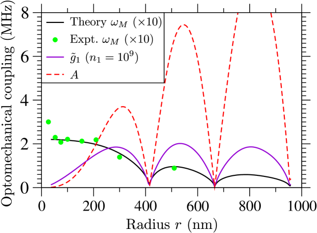
Figure 1: (Colour online) Size dependent effects in the magnitude of the optomechanical coupling parameter ${\tilde{g}}_{1}$. It is assumed that cavity parameters would correspond to ${\tilde{g}}_{1}=10^{6}$ Hz at $r=150$ nm, for photon numbers $n_{1}=10^{9}$. For comparison, the value of $A$ is also shown, as are the experimental and simulated frequencies $\omega_{a}\equiv\omega_{M}=2\pi f_{M}$. The $\omega_{M}$ are scaled by a factor of 10 for clarity and in fact, values of $\omega_{M}\sim 1$ MHz are quite realistic in optical cavities.

2 Towards strong light-matter coupling with two optical cavity modes

The Hamiltonian in Eq. 6 appears analogous in form to standard, well-studied optomechanical Hamiltonians, albeit with two optical modes rather than one. However, it differs in one important respect: in this case, both the mechanical frequency $\omega_{M}(\Delta_{1}^{x},\Delta_{2}^{x})$ and the optomechanical coupling strengths $g_{1,2}\equiv g_{1,2}(\Delta_{1}^{x},\Delta_{2}^{x})$ are not fixed and depend on the detunings. The fact that the frequencies of the three modes (two optical, one mechanical) are interdependent makes the dynamics different from other optomechanical set-ups, where the equilibrium mechanical frequency (i.e. excluding shifts arising from the fluctuations) is intrinsic to the mechanical oscillator.

There is considerable interest in achieving strong-coupling, which leads to regimes of light-matter hybridization. The corresponding mode splitting has been observed experimentally [24]. In typical set-ups, these regimes are reached if the rescaled effective optomechanical coupling exceeds the damping rates i.e. ${\tilde{g}}=g\sqrt{n}\gtrsim\kappa,\Gamma_{M}$, where $n\sim|\alpha|^{2}$ is the cavity photon number. Even if the unnormalized coupling is weak, strong-coupling regimes may be achieved by increasing the driving power and thus increasing intracavity photon numbers.

In the present levitated system, a particularly interesting regime would involve triple-mode hybridization enabling, for example, the coupling of the two modes of light via the mechanical mode. However, here, mode hybridization (for which ${\tilde{g}}_{1,2}=g_{1,2}\alpha_{1,2}\gtrsim\kappa,\Gamma_{M}$) depends non-trivially on the detunings.

We argue that large coupling cannot be easily achieved by increasing the driving power, since ${\tilde{g}}_{1,2}\propto n_{1,2}^{1/4}$ and thus increases slowly with the driving strength. We can show, by a simple argument, that increasing the nanosphere size provides the most effective means to attain strong coupling.

For the self-trapped system, optomechanical coupling strengths are $g_{j}=\sqrt{2}kAX_{zpf}\sin 2(kx_{0}-\phi_{j})$ and depend on the detunings via $x_{0}$. Note also that $X_{zpf}=\sqrt{\hbar/(2m\omega_{M})}$ here too depends on the detunings via $\omega_{M}$.

For triple mode hybridization, $\omega_{M}\sim\Delta_{1}\sim\Delta_{2}$. For convenience, we also take $\phi_{1}=0,\phi_{2}=\pi/4$. Then, since $\tan 2kx_{0}={|\alpha_{2}|^{2}}/{|\alpha_{1}|^{2}}$, we can re-write Eq. 5:

$$\omega_{M}^{2}=\frac{2\hbar Ak^{2}}{m\cos{2kx_{0}}}|\alpha_{1}|^{2}.$$ (7)

We consider near symmetric driving of the two optical modes for which $R\sim 1$ and thus $kx_{0}\approx\phi/2=\pi/8$ so $\omega_{M}\sim\left({\frac{2\hbar Ak^{2}}{m}}\right)^{1/2}n_{1,2}^{1/2}$. Hence,

$${\tilde{g}}_{1,2}\sim\left({\frac{\hbar k^{2}}{4}}\right)^{1/4}\left(\frac{A^{3}n_{1,2}}{m}\right)^{1/4}.$$ (8)

Since the optomechanical coupling increases only very slowly with cavity photon number the most effective means to reach strong coupling regimes is to increase the nanosphere size to the maximum practical value ($r\sim 200-250$ nm).

For the ideal case where the nanosphere radius $r$ is small [19] ie. $\lambda\gg r$, then $A(r\ll\lambda)\equiv A_{0}(r)$ where the small nanosphere coupling takes the form:

$$A_{0}(r)=\frac{3}{2}\frac{\epsilon_{r}-1}{\epsilon_{r}-2}\frac{V_{s}}{V_{c}}\omega_{L}$$ (9)

where $V_{s}=4/3\pi r^{3}$ is the sphere volume (and hence $m=V_{s}\rho$ where the density $\rho=2000$ Kg m^-3 for silica). In turn, $V_{c}=\pi(w/2)^{2}L$ is the cavity volume, where $w\approx 40\,\mu$m is the cavity waist and $L\simeq 0.5-1$ cm is the cavity length.

For larger nanospheres, the measured size-dependent corrections must be applied. In the experiments described below, we find that the mechanical oscillation frequency is modulated by a finite size correction $\omega_{M}(r)=\omega_{M}(r\simeq 0)f(r)$ (see Fig. 11 and description of the measurement of $f(r)$ in section 5 below). Thus, since:

$$\omega_{M}^{2}\propto\frac{A(r)}{m},$$ (10)

then $A(r)\equiv A_{0}(r)f^{2}(r)$ and the coupling is in turn modulated by the finite size correction. The experimental results suggest that for $r\lesssim 200$ nm, then $f(r)\sim 1$ and $A(r)\simeq A_{0}(r)$.

For example, for $r=150$ nm, $L=1$ cm and $w=40\,\mu$m, then $A_{0}\simeq 8\times 10^{5}$ Hz. For reasonable values of cavity decay constants $\kappa\simeq 2-8\times 10^{5}$ Hz, then for $n_{1}\sim 10^{9}$,

$${\tilde{g}}_{1,2}\sim 5.4\times 10^{-6}\left({\frac{A^{3}n_{1,2}}{m}}\right)^{1/4}\simeq 10^{6}\,\mathrm{Hz}\gg\kappa$$ (11)

For $r\lesssim 200$ nm, ${\tilde{g}}_{1,2}\propto r^{3/2}$. Thus a 200 nm sphere provides an optomechanical coupling about an order of magnitude larger than a 40-50 nm sphere. To achieve a comparable increase in coupling by photon number enhancement would require increasing the driving power by a factor of order $10^{4}$.

A more careful analysis, including the effects of the finite-size correction function $f^{2}(r)$ is shown in Fig. 1. We see that ${\tilde{g}}_{1}$ (and for $n_{1}\sim n_{2}$, also ${\tilde{g}}_{2}$) reaches a maximum value for $r\simeq 300$ nm before falling to zero. Other maxima for larger $r$ do not provide a larger value of ${\tilde{g}_{1,2}}$. Furthermore, they have the disadvantage that they may enhance photon recoil heating effects. For comparison, the value of $A$ is also shown, overlaid on the experimental and simulated frequencies.

3 Dynamics

3.1 Optomechanical damping

A previous study [23], using rescaled coordinates, investigated the full parameter space of two optical mode cooling. Here we investigate more carefully the effect of non-zero mechanical damping. Using linear response theory, we can extract cooling rates from the equations Eq. 4:

$$\Gamma_{opt}=\left[S_{1}(\omega_{M})+S_{2}(\omega_{M})-S_{1}(-\omega_{M})-S_{2}(-\omega_{M})\right],$$ (12)

where

$$S_{j}(\omega)=\frac{|\alpha_{j}|^{2}g^{2}_{j}\kappa}{[\Delta_{j}^{x}-\omega]^{2}+\frac{\kappa^{2}}{4}},$$ (13)

for $j=1,2$. Net cooling occurs for $\Gamma_{opt}<0$. Although the above is quite similar in form to standard optomechanical expressions, as explained previously, rather different behaviour is observed since here $\omega_{M}$ and $g_{j}$ are both dependent on the $\Delta_{j}^{x}$.

From quantum perturbation theory we can show that $R_{n\to m}$, the rate of transition from state $n$ to $n+1$ is: $R_{n\to n+1}=(n+1)\left(S_{1}(\omega_{M})+S_{2}(\omega_{M})\right)$ while $R_{n\to n-1}=n\left(S_{1}(-\omega_{M})+S_{2}(-\omega_{M})\right)$

For $n>>1$, then $R_{n\to n+1}-R_{n\to n-1}$ gives the cooling rate of Eq.12. However, with the exact expressions we can show that the equilibrium mean phonon number is

$$\langle n\rangle_{PT}=\frac{S_{1}(\omega_{M})+S_{2}(\omega_{M})}{S_{1}(-\omega_{M})+S_{2}(-\omega_{M})-S_{1}(\omega_{M})-S_{2}(\omega_{M})}.$$ (14)

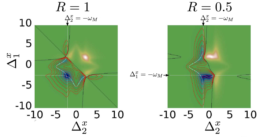
Figure 2: (Colour online) Maps of cooling rates calculated from Eq. 12 for parameters $R=1.0$ and $R=0.5$. Blue corresponds to cooling, yellow/white to heating. The white lines indicate the locus of the single field resonances (where $-\Delta_{1}^{x}=\omega_{M}$ or where $-\Delta_{2}^{x}=\omega_{M}$). The detunings are given in units of $A$ and are dimensionless. For $R=1$ it is clear that there is a deep, maximum cooling region at a double resonance where the two white lines intersect and both optical fields cool simultaneously. It is also evident that there is a strong cooling resonance for $+\Delta_{1,2\pm}^{x}=\omega_{M}$. For $R=0.5$, three cooling resonances $-\Delta_{1\pm}^{x}=\omega_{M}$, $-\Delta_{2\pm}^{x}=\omega_{M}$ and $+\Delta_{1}^{x}=\omega_{M}$ merge to give a very broad strong-cooling region, quite insensitive to detuning $\Delta_{2}$ over a range of over 1 MHz. Here $A=\kappa/2=0.3$ MHz and the input power into mode 1 corresponds to 2 mW.

In Fig. 2 we show colour maps comparing the cooling and minimum phonon numbers for both $R=0.5$ and $R=1$ respectively. The cooling behaviour was investigated previously in [23]. In this case, for each fixed detuning $\Delta_{1}$ there are up to three cooling resonances (at three different values of $\Delta_{2}$), where strong damping is observed (and similarly for each fixed $\Delta_{2}$). This is in contrast to single optical mode schemes where there is a single cooling resonance for which $\Delta_{1}=-\omega_{M}$ or $\Delta_{2}=-\omega_{M}$. For the $R=0.5$ map the three cooling resonances merge, giving a single extended cooling region of about 1 MHz width.

For $R=1$ the map has a high degree of symmetry, since the role of the two optical modes is interchangeable. The figures show that the largest cooling rates are found in the double resonance region, making it the most favourable region to work in.

The equilibrium phonon number in Eq. 14 concerns only the idealised situation where there is a very good vacuum, negligible photon recoil heating and thus no mechanical damping or heating effects. For small $r\lesssim 200$ nm spheres, we assume recoil heating is negligible [19] and the dominant source of mechanical damping is background gas collisions, which provide an effective mechanical damping $\Gamma_{M}=\frac{8}{3}\pi\frac{m_{g}}{m_{s}}r^{2}n_{g}\bar{v}_{g}$ [18, 19] where $m_{g}/m_{s}$ is ratio of the gas particle’s mass to that of the sphere, $n_{g}$ is the gas number density and $\bar{v}_{g}$ is the mean gas velocity for a room temperature thermal distribution.

It can be shown that the perturbation theory argument above can be adapted to obtain equilibrium phonon numbers for a given cooling rate $\Gamma_{opt}$:

$$\langle{n}\rangle_{PT}=\frac{\frac{k_{B}T_{B}}{\hbar\omega_{M}}{\Gamma_{M}}+\left[S_{1}(\omega_{M})+S_{2}(\omega_{M})\right]}{\Gamma_{M}+|\Gamma_{opt}|},$$ (15)

where $T_{B}\simeq 300$K. Alternatively, the final equilibrium temperatures $T_{eq}=\frac{\Gamma_{M}T_{B}+|\Gamma|T_{vac}}{\Gamma_{M}+|\Gamma|}$, where $T_{vac}$ is the equilibrium oscillator temperature which would have been obtained in a perfect vacuum.

3.2 Quantum and semiclassical noise spectra

Although we investigate only a two optical mode system, generalization to more optical modes is straightforward. We consider a set of equations of motion, for $j=1,...N$:

$${\dot{\hat{b}}} = -(i\omega_{M}(\Delta_{1}^{x},...\Delta_{j}^{x})+\frac{\Gamma_{M}}{2}){\hat{b}}+i\sum_{j}g_{j}(\Delta_{1}^{x},...\Delta_{j}^{x})({\hat{a}}_{j}+{\hat{a}}_{j}^{\dagger})+\sqrt{\Gamma_{M}}{\hat{b}}_{in}$$

$${\dot{\hat{a}}_{j}} = (i\Delta_{j}^{x}-\frac{\kappa}{2}){\hat{a}}_{j}+ig_{j}(\Delta_{1}^{x},...\Delta_{j}^{x})\alpha_{j}({\hat{b}}+{\hat{b}}^{\dagger})+\sqrt{\kappa}{\hat{a}}_{in}^{(j)},$$

where the optomechanical strengths $g_{j}(\Delta_{1}^{x},...\Delta_{j}^{x})=-kAX_{ZPF}\sin 2(kx_{0}-\phi_{j})$ depend on the detunings (as does the mechanical frequency $\omega_{M}$). In the two mode case we consider, we take $\phi_{1}=0$ and $\phi_{2}=\pi/4$.

The optical modes are subject to photon shot noise, while the mechanical modes are subject to Brownian noise from collisions with gas molecules in the cavity. For the photon shot noise, we assume independent lasers and uncorrelated zero temperature noise for which $\langle{\hat{a}}_{in}^{\dagger}(t^{\prime}){\hat{a}}_{in}(t)\rangle=0$, while $\langle{\hat{a}}^{(i)}_{in}(t^{\prime}){\hat{a}}^{(j)\dagger}_{in}(t)\rangle=\delta(t-t^{\prime})\delta_{ij}$. For the gas collisions, we take $\langle{\hat{b}}_{in}(t^{\prime}){\hat{b}}_{in}^{\dagger}(t)\rangle=(n_{B}+1)\delta(t-t^{\prime})$ and $\langle{\hat{b}}_{in}^{\dagger}(t^{\prime}){\hat{b}}_{in}(t)\rangle=n_{B}\delta(t-t^{\prime})$ where the number of surrounding bath phonons $n_{B}\approx\frac{k_{B}T}{\hbar\omega_{M}}$.

The above equations can be integrated in frequency space to obtain analytical expressions for the displacement noise spectra for the arbitrary mode case. We can evaluate the displacement spectrum $S_{xx}(\omega)\equiv\langle|x(\omega)|^{2}\rangle_{QM}=\frac{1}{2\pi}\int e^{-i\omega\tau}\langle x(t+\tau)x(t)\rangle d\tau$. We obtain:

$$\langle|x(\omega)|^{2}\rangle_{QM}|M(\omega)|^{2} = {\Gamma_{M}}\left[|\chi_{M}(\omega)|^{2}n_{B}+|\chi_{M}(-\omega)|^{2}(n_{B}+1)\right]$$ (17)

$$+ \frac{\kappa}{2}|\mu(\omega)|^{2}\sum_{j=1,2}g_{j}^{2}|\chi_{jo}(-\omega)|^{2},$$

where the $\chi(\omega)$ represent optical and mechanical susceptibilities:

$$\chi_{jo}(\omega)=\left[-i(\omega+\Delta_{j}^{x})+\frac{\kappa}{2}\right]^{-1};\ \chi_{M}(\omega)=\left[-i(\omega-\omega_{M})+\frac{\Gamma_{M}}{2}\right]^{-1}.$$ (18)

with $\mu(\omega)=\chi_{M}(\omega)-\chi_{M}^{*}(-\omega)$ and $\eta_{j}(\omega)=\chi_{jo}(\omega)-\chi_{jo}^{*}(-\omega)$; then also $M(\omega)=1+\mu(\omega)\sum_{j}g_{j}^{2}|\eta_{j}(\omega)|^{2}$.

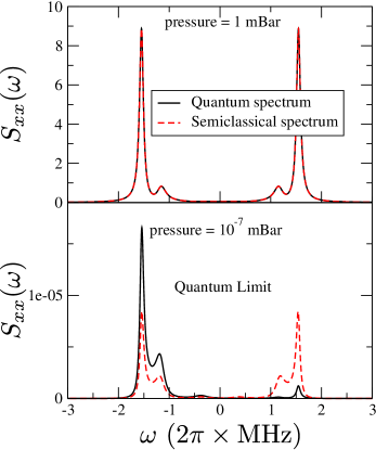
Figure 3: (Colour online) Comparison between quantum and semiclassical displacement spectra for gas pressures of 1 mBar and at near vacuum pressure in a strong cooling region. At high vacuum, the ground state is approached and thus, for the quantum spectrum, the blue sideband vanishes. At higher pressure there is good agreement between the quantum and classical results. Spectra near double resonance for input power $P_{1}=7$ mW, $A=\kappa=3\times 10^{5}$ Hz, $\Delta_{1}=-1.5$ MHz, $\Delta_{2}=-0.68$ MHz, $R=0.5$. Some hybridization between the mechanical mode and optical mode 1 is seen in the characteristic double-peak sideband structure.

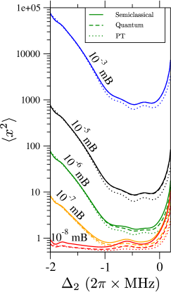
Figure 4: For the broad cooling region formed from three overlapping resonances seen in Fig. 2(b), we show equilibrium phonon numbers obtained from Eqs. (15), (17) and (20) i.e. perturbation theory, the analytical quantum noise formula and semiclassical Langevin equations respectively. Agreement between quantum and semiclassical results is excellent, less so for perturbation theory at low pressures.

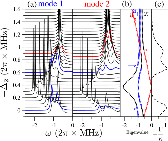
Figure 5: Triple mode splitting. For $A=\kappa=3$ MHz, even at quite high pressures (here 1 mBar), mode splitting is seen in the noise spectra of the optical modes. In all the plots, $\Delta_{1}=-1.15$ MHz is held fixed while $\Delta_{2}$ is swept from 0 to -1.6 MHz (for an input power of 2 mW into mode 1, while $R=0.5$). (a) Shows noise spectra for both optical mode 1 and mode 2. Three way hybridization between the mechanical and both optical modes appears clearly (highlighted in the bold blue line). For clarity, some of the strongest peaks have been truncated in height. In (b) three avoided crossings are apparent. The dominant character of each normal mode is indicated by the colour (black is mechanical, blue is optical mode 1, red is optical mode 2). When $-\Delta_{2}$ is large, there is no mixing. However as $\Delta_{2}\to 0$, there is strong mixing and the dominant character of each normal mode changes from light to matter (or vice versa) as an avoided crossing is encountered. Panel (c) shows the cooling and indicates strong cooling at each of the avoided crossings.

We compare the quantum displacement with corresponding semiclassical solutions in the steady state. The linearised two mode system Eq. 6, in matrix form corresponds to a standard problem [30]. Inclusion of the noise arising from gas collisions or laser shot noise yields a set of corresponding Langevin equations: $\frac{d{\bf X(t)}}{dt}={\bf A}{\bf X}+{\bf BE}(t)$, where ${\bf A}$ is termed the drift matrix. Its eigenvalues give the stabilities and eigenfrequencies of the system’s normal modes, while the noise is determined by ${\bf B}$, a constant diagonal matrix. The elements of the random noise matrix are assumed to be $\delta$-correlated $\langle E_{i}(t)E_{j}(t^{\prime})\rangle=\delta(t-t^{\prime})\delta_{ij}$. Methods for obtaining the solution for the steady state correlation functions of this system, under conditions of stability, i.e. where all the eigenvalues of ${\bf A}$ have negative real parts, are well-known [30]. The required noise spectra, or autocorrelation functions, in frequency space are:

$${\bf S}(\omega)=\frac{1}{2\pi}_{-\infty}\int^{\infty}e^{-i\omega\tau}\langle{\bf X}(t+\tau){\bf X^{T}}(t)\rangle d\tau,$$ (19)

where,

$${\bf S}(\omega)=\frac{1}{2\pi}\left({\bf A}+i\omega{\bf I}\right)^{-1}{\bf B}{\bf B^{T}}\left({\bf A^{T}}-i\omega{\bf I}\right)^{-1},$$ (20)

where the diagonal matrix ${\bf B}{\bf B^{T}}$ has elements $\left((n_{B}+\frac{1}{2}){\Gamma_{M}},(n_{B}+\frac{1}{2}){\Gamma_{M}},\frac{\kappa}{2},\frac{\kappa}{2},\frac{\kappa}{2},\frac{\kappa}{2}\right)$. From the above, the noise spectra of all modes may be calculated. Eq.SSC yields semiclassical sideband spectra, symmetrical in $\omega$.

In Fig. 3, we compare semiclassical displacement spectra calculated from Eq. 20 with corresponding quantum results obtained from Eq. 17. At high pressures (and hence high phonon occupancy) there is excellent agreement between semiclassical and quantum results. At low pressures (near ground state cooling) however, the quantum spectrum shows a characteristic asymmetry, such as was observed recently in experiments on photonic cavities [12].

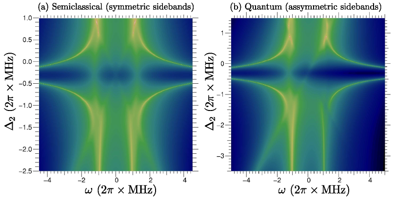
Figure 6: Maps of the displacement noise spectra $S_{xx}(\omega)$, showing mode splitting for similar parameters to Fig. 3, near the quantum limit, except that here $\Delta_{1}=-1.5$ MHz is held fixed while $\Delta_{2}$ (vertical axes) is swept. (a) Shows the semiclassical spectrum which is symmetric in frequency $\omega$. (b) Shows the quantum spectrum which is asymmetric. In both cases, triple hybridization appears clearly and is seen near $\Delta_{2}\approx-1.0$ MHz. (c) shows the corresponding behaviour for $A=\kappa/2$, showing that the triple peak structure has disappeared. Note that $\log{S_{xx}(\omega)}$ is plotted.

3.3 Comparison between perturbation theory, semiclassical and quantum results

The equilibrium variance (and hence the final phonon number) of the mechanical oscillator is,

$$\langle x^{2}\rangle=\frac{1}{2\pi}_{-\infty}\int^{\infty}\langle|x(\omega)|^{2}\rangle d\omega,$$ (21)

thus, the final equilibrium temperature of the mechanical oscillator after optomechanical cooling is $k_{B}T_{eq}=1/2m\omega_{M}^{2}\langle X^{2}\rangle$. Noting the rescaling $\langle X^{2}\rangle=2X_{ZPF}\langle x^{2}\rangle$ and setting $k_{B}T_{eq}=(\langle n\rangle+1/2)\hbar\omega_{M}$, we can write $\langle x^{2}\rangle=\langle n\rangle+1/2$.

Using Eqs. (LABEL:QM), (20) and (15), we can investigate final equilibrium phonon numbers (and the minimum achievable for levitated self-trapped spheres) comparing quantum, semiclassical and perturbation theory respectively. In Fig. 4, we compare the corresponding equilibrium phonon numbers, $\langle n\rangle_{QM}$, $\langle n\rangle_{SC}$ and $\langle n\rangle_{PT}$ respectively for the unusual triple cooling resonance region shown in Fig. 2. Cooling to near the ground state $\langle n\rangle\sim 0$ is possible for a pressure of order $10^{-6}$ mBar, even for modest driving powers of 2 mW and values of $A\simeq 3\times 10^{5}$ Hz corresponding to spheres of order $r\simeq 100$ nm.

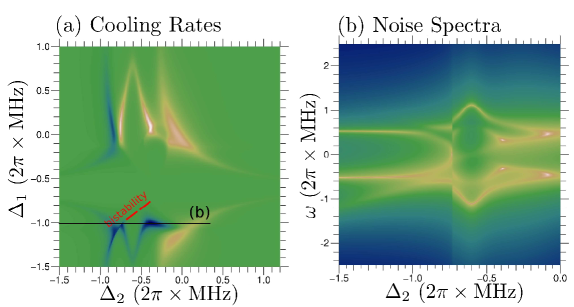
Figure 7: Mode mixing and bistability for $A=3\kappa=6\times 10^{5}$ Hz. We consider a relatively low input power of 0.37 mW. (a) plots the optomechanical cooling rate (blue indicates cooling, brown indicates heating). The red dashed line indicates the locus of bistability as a function of the detunings $\Delta_{1}$ and $\Delta_{2}$. The discontinuity in the cooling can be discerned near the strong doubly resonant cooling region. (b) shows displacement noise spectra $S_{xx}(\omega)$ as a function of $\omega$ plotted along $\Delta_{1}=-1$ MHz (along black horizontal line in upper panel). We sweep in increasing $\Delta_{2}$. At the point where $\Delta_{1}=-1$ MHz intersects the bistability, a discontinuity in the noise spectra is apparent. On one side of the discontinuity there is strong hybridization between the mechanical mode and optical mode 2; this changes abruptly across the discontinuity to hybridization between the mechanical mode and optical mode 1 for larger $\Delta_{2}$. This may allow for control of entanglement between the modes. The map corresponds to near-vacuum conditions so the system is near the quantum ground state in this regime (as evidenced by the asymmetric sidebands).

4 Strong coupling regimes: triple mode splitting and bistability

The multimode, or at least two mode, self-trapping regime may permit new possibilities for position sensing and for controlling entanglement between two optical modes and the mechanical resonator. Here we investigate regimes where such effects are clearly apparent. The implications of the measurement for the accessible range of optomechanical coupling strengths suggests that multiple hybridization and bistability are quite accessible with reasonable cavity parameters.

In Fig. 5 we investigate the complex behaviour of the eigenmode frequencies of the self-trapped, levitated system. On the left panels (Fig. 5 (a)) we plot the noise spectra of the two optical modes, which exibit sidebands near $\omega\simeq\omega_{M}$ since the corresponding optical fields are modulated by the motion of the mechanical oscillator. Here we fix one detuning ($\Delta_{1}=-1.15$ MHz) and look at the behaviour as the other detuning is varied. The sidebands are displaced in frequency and split: one effect is simply due to the dependence of $\omega_{M}$ on $\Delta_{j}$ (unique to the levitated system); it arises from the calculation of the equilibrium fields and frequencies. The other effect is due to normal mode mixing (hybridization of light and matter modes) arising from the linearised equations. If $\omega_{M}\simeq\Delta_{1}\simeq\Delta_{2}$ simultaneous hybridization is observed, provided ${\tilde{g}}_{1,2}\gtrsim\kappa$. Figure 5 (b) shows that there are several distinct avoided anti-crossings, where the dominant character of each eigenmode changes; if two crossings coincide, the spectra show a characteristic triple-peak structure (symmetric about $\omega=0$ in the semiclassical regime shown here). Panel (c) shows that the corresponding cooling rate is enhanced at each avoided level crossing.

In Fig. 6 we plot displacement spectra corresponding to Fig. 3, but over a range of values of $\Delta_{2}$. A log-scale is used for $S_{xx}(\omega)$. The triple mixing which can appear when two avoided crossings nearly coincide is clearly apparent at $\Delta_{2}\simeq 1$ MHz.

Static bistability in a cavity of varying length has been seen experimentally [31]. The potential for generating entanglement has recently been investigated in an optomechanical system [32]; however, a relatively high laser power $P\sim 50$ mW is required.

For the self-trapped systems, the incoherent sum of the optical standing-wave potentials $\cos^{2}(kx-\phi_{1})$ and $\cos^{2}(kx-\phi_{2})$ does not by itself produce a double-well structure; nevertheless, as we see below, in combination with optomechanical shifts, bistabilities are observed, even for weak driving. Whether a double-well structure emerges, or not, is completely independent of the driving power (where $P\propto E_{1}^{2}$) and can emerge at very low input powers, as we demonstrate below. It is easy to see that the levitated particle moves in an effective static potential $V(x)$ where:

$$\frac{dV(x)}{dx}=\hbar kAE_{1}^{2}\left[\frac{\sin 2(kx-\phi_{1})}{|(\kappa/2)-i\Delta_{1}(x)|^{2}}+R^{2}\frac{\sin 2(kx-\phi_{2})}{|(\kappa/2)-i\Delta_{2}(x)|^{2}}\right],$$

(22)

and

$$V(x)=\hbar AE_{1}^{2}\left[\tan^{-1}\left({\frac{\Delta_{1}(x)}{\frac{\kappa}{2}}}\right)+R^{2}\tan^{-1}\left({\frac{\Delta_{2}(x)}{\frac{\kappa}{2}}}\right)\right].$$

(23)

Here, note that the shifted detuning $\Delta_{j}(x)=\Delta_{j}+A\cos^{2}(kx-\phi_{j})$ is dependent on $x$, not the equilibrium displacement $x_{0}$. This potential admits two stable equilibrium points over parameter regimes where $A\gg\kappa$ (in practice, such bistability is observed already for $A/\kappa\simeq 3$). It is evident that the driving power factors out, so does not affect the shape of the potential, providing only a scaling factor. We show in Fig. 7 that for a high $A/\kappa$ ratio simultaneous hybridisation and bistability co-exist: we show that that for $P=0.37$ mW , $A=3\kappa$ , $R=0.15$ and modest photon numbers $n_{1}\sim 10^{8}$ we can switch discontinuously from hybridisation between the mechanical mode and optical mode 1, to hybrization between the mechanical mode and mode 2. We take $\phi_{1}=0,\phi_{2}=\pi/4$. In the noise spectra, the switch is heralded by a large zero-frequency peak in the displacement spectra, which is clearly apparent in Fig. 7.

5 Experiment

5.1 Current experimental status: Loading protocols and variation of trap frequency with radius

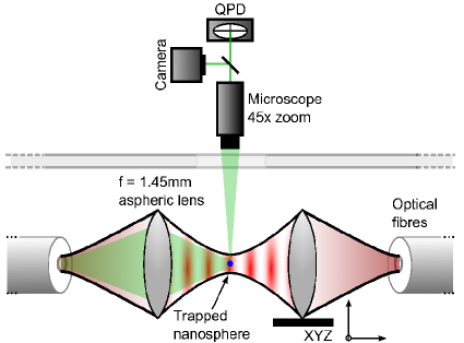
Figure 8: (Colour online) Schematic diagram of the standing wave trap. It is formed from two counter-propagating 1064 nm beams focused inside a vacuum chamber. Light at 532 nm enters via one fibre to image the sphere. Images and measurement of the axial and transverse position of the trapped nanosphere as a function of time are measured by a CCD camera and quadrant cell photodiode (QPD) respectively, through a long working distance microscope outside the vacuum chamber.

We have built a simple standing wave dipole trap to develop protocols for loading a single nanosphere into the trap to confirm that nanospheres with a range of radii around 100 nm can be trapped. Importantly, we have measured the variation in trap frequency with sphere radius so that realistic values of optomechanical coupling strengths, for a given nanosphere radius, can be included in our models. In this section we explain how the size-dependent modulation function $f(r)$, used in the theory section above to obtain $A(r)$ and the optomechanical coupling strengths, was measured.

A schematic of the standing wave trap used in our experiments is shown in Fig. 8. The standing wave trap consists of two focused beams that counter-propagate and overlap near their foci. The two laser beams, derived from the same laser at a wavelength of 1064 nm, enter the trapping region via optical fibres. The light exiting the fibres is focused using aspheric lenses (Thorlabs C140TME) with a focal length of 1.45 mm and numerical aperture 0.55. The power in each trapping beam after it has passed through each lens is measured to be $150\pm 10$ mW, and the best focused beam waist (radius) is theoretically 1.7 $\mu$m. To optimize the alignment of the trap, we maximize the light through-coupled from one fibre into the other. This is accomplished by mounting one optical fibre and its aspheric lens on an XYZ flexure stage. The alignment is done inside the vacuum chamber at atmospheric pressure.

A long working distance microscope (Navitar Zoom 6000 system, with up to 45x zoom) is used to image the trapped sphere. The image is split into two using a beamsplitting plate, with one image directed to a CCD camera for diagnostics and the other aligned onto a quadrant cell photodiode (QPD) which measures position fluctuations as a function of time in two orthogonal axes. We define the axial direction as that along which the trapping light propagates, and the transverse direction as the orthogonal axis in the focal plane of our imaging system. Light at 532 nm is used to illuminate the trapped sphere, as the QPD is more sensitive at this wavelength. The green beam enters the system via one of the optical fibres, as shown in Fig. 8, and a filter is used to stop 1064 nm light reaching the detectors. The power of the 532 nm beam is 10 mW.

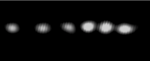
Figure 9: An image of a string of 100 nm diameter beads trapped in the standing wave trap. A single bead is trapped by continually blocking and unblocking one of the trapping beams until only one sphere is trapped.

Silica (SiO₂) nanospheres, manufactured by Microspheres-nanospheres and Bangs Laboratories, are introduced into the trapping region at atmospheric pressure via an ultrasonic nebulizer (Omron NE-U22). These spheres range in radius from 26 nm to 510 nm and are suspended in methanol. The nanosphere solution is sonicated using an ultrasonic bath for at least an hour before trapping to prevent clumping. Once introduced into the trapping region the methanol surrounding the spheres rapidly evaporates and the spheres are trapped over many fringes of the standing wave, as shown in Fig. 9. As our imaging system does not have single fringe resolution we cannot determine if more than one sphere is trapped in a single fringe by this method. However, this information can be inferred from the relative intensity of the light scattered from the trapped spheres and also by the reduced stability of the particles in the trap when more than one particle is trapped. To reduce the number of trapped particles the trapping light is briefly blocked and unblocked. This is repeated until a single sphere is visible in the trap. At this pressure, where there is a strong damping force from air the sphere can be held in the trap indefinitely.

To measure the trap frequency the air is pumped from the system, and at this point no more spheres enter the trap, as without air-damping their velocity is too high. The air pressure in the trap is reduced to 5 mbar, so that clear trap frequencies can be obtained from the power spectrum of the position fluctuations of the trapped sphere, as recorded on the QPD. Example power spectra are shown in Fig. 10. Above 5 mbar the damping of the motion in the trap due to air broadens the peak in the power spectrum so that finding an accurate trap frequency is difficult. Below pressures of 5 mbar the spheres become unstable in the trap and escape. This is most likely due to radiometric forces which have been compensated for in other experiments using feedback techniques [25, 26]. At 5 mbar the damping rate due to gas collisions is significantly less than our lowest measured trap frequencies, and thus the measured frequency at this pressure is a good approximation to the bare trap frequency which would be measured in vacuum without damping.

The angular axial trap frequency for a small polarizable particle in a standing wave is $\omega_{a}=2\pi f_{a}=\sqrt{\frac{4\alpha k^{2}I_{0}}{m\epsilon_{0}c}}$, where the polarizability of a sphere of refractive index $n$ is $\alpha=4\pi\epsilon_{0}r^{3}\frac{n^{2}-1}{n^{2}+2}$. The maximum intensity in the radial center of each equal intensity beam is given by $I_{0}$, and $k$ is the magnitude of the wavevector of each beam. The sphere has mass $m=4/3\pi\rho r^{3}$, radius $r$ and density $\rho\simeq 2000$ kg m^-3. The transverse trap frequency is given by $\omega_{t}=\sqrt{\frac{8\alpha I_{0}}{m\epsilon_{0}cw^{2}}}$, where $w$ is the focused spot size (radius) of the two counter-propagating beams. From these expressions the ratio of the trap frequencies is given by $\omega_{a}/\omega_{t}=kw/\sqrt{2}$.

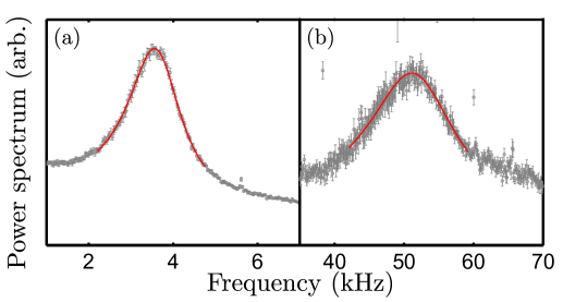
Figure 10: (Colour online) Power spectra at 5 mbar calculated from a measurement of the position of a trapped 200.1 nm diameter nanosphere as a function of time, using a QPD. (a) The transverse frequency, and (b) an axial frequency. Outlier points are due to electronic noise. Red lines show fitted Gaussian functions, from which the trap frequencies are extracted.

The trap frequencies in each axis are determined by fitting measured position fluctuation power spectra using $\frac{2k_{B}T}{m}\frac{\Gamma_{0}}{(\omega_{a}^{2}-\omega^{2})^{2}+\omega^{2}\Gamma_{0}^{2}}$, where $k_{B}$ is Boltzmann’s constant and $\Gamma_{0}$ is the damping rate. The fit to the data is shown in Fig. 10 with $\Gamma_{0}/2\pi\simeq 2.4$ kHz for the axial trap frequency. Several sets of data were taken for different spheres of the same nominal radius and the measured axial and transverse trap frequencies for each size sphere are shown in Fig. 11. The derived trap frequencies for each sphere radius are the average over different experiments at each radius, and the errors are the standard errors in the mean. The uncertainty in the sphere radius is taken from the information supplied by the manufacturer. Two axial (red and green data in Fig. 11) frequencies and one transverse frequency (blue data points) were measured. When a particle is tightly trapped by the optical field only one axial frequency is expected from a single sphere in a standing wave. The lower axial frequency (in green in figure 11) is always observed in the data and this is taken as the true axial frequency. The higher frequency, which is often present in the data, may be due to the trapping of two spheres in a single anti-node, with the higher frequency occurring due to optical binding, which requires further study [27]. The higher axial frequency also changes rapidly with sphere size, indicating that it is not the true axial trap frequency, which should be almost constant for the small spheres. The presence of a single axial frequency is, we believe indicitave of having trapped a single sphere.

Although we don’t know the radial dimensions of the beam within the trap we can estimate this value from the ratio of the axial to transverse trap frequencies for small spheres. The spot size from this ratio is $w=\frac{\sqrt{2}}{k}\frac{\omega_{a}}{\omega_{t}}$ and for $\frac{\omega_{a}}{\omega_{t}}$=9.8 this gives a spot size of $w=2.3\,\mu$m. Since the trap frequency with two overlapping beams of size 2.3 $\mu$m would be equal to 207 kHz with a power in each beam of 150 mW, and we only measure a maximum axial trap frequency of approximately 40 kHz, we conclude that the particles are trapped in a standing wave formed where the waist of one beam is much larger. If one spot size is 2.3 $\mu$m the other would have to be 15 $\mu$m. A plot of the calculated axial trapping frequency, found by calculating Maxwell’s stress tensor ([28, 29]), is also shown in Fig. 11. Like the experimental data the trapping frequency is constant for small spheres and decreases to approximately zero when the particle size is comparable to the size of the interference pattern produced by the standing wave. At larger radii the force on the particle changes sign and a stable trap is formed in a node of the standing wave, as shown for the particle of radius 510 nm. Our measurements confirm that for particle radii less that 200 nm the simple dipole model for the nanospheres is adequate for modelling the cooling and dynamics of the nanospheres in an optical cavity utilising 1064 nm radiation.

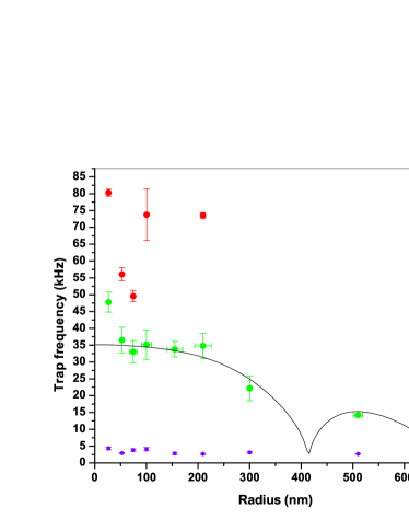
Figure 11: (Colour online) Measured trap frequencies as a function of sphere radius. Points plotted in green are the axial trap frequency, blue are the transverse trap frequency and the red data points are the higher axial trap frequencies which are believed to be due to optical binding. The solid black line is a theoretical curve derived from a numerical calculation [28].

Our experiments have shown that optical traps without feedback are currently limited to operation at pressures down to a few millibar for all particles that we have measured. In addition this limiting pressure did not change by reducing the intensity by 50%. This radiometric force is due to localized heating of nanosphere and the subsequent heating of the surrounding air. At low pressures, when the mean free path is comparable to the size of the nanosphere, the radiometric force competes with and eventually dominates the dipole force which traps the particle. While feedback techniques have been successful [26], decreasing the absorption of the nanospheres is another route to minimising radiometric effects. This is feasible since all the spheres we have used in this study are not made of optical quality glass but from colloidally grown nanospheres. Finally, we have also successfully trapped silica spheres in an ion trap at pressures of $10^{-6}$ mbar which could be used to load an optical trap formed by a cavity at lower pressures where radiometric forces are not significant.

Conclusions

We have described a study of the dynamics and noise spectra of self-trapped levitated optomechanical systems. We have been able to show, by combining experimental measurements and theoretical calculations that strong light-matter coupling is attainable over a wide range of particle sizes, and that these can be trapped. The interdependence of the mechanical and optical mode frequencies, unique to self-trapped levitated systems provides a complex and interesting side-band structure, including multi-mode mixing and bistabilities which we aim to explore experimentally. These conclusions are supported by measurements of trap frequency made in an optical standing trap where we have demonstrated a protocol for loading a single nanosphere in a single antinode.

Acknowledgements: We acknowledge support for the UK’s Engineering and Physical Sciences Research Council.

References

References

- [1] F. Marquardt and S Girvin, Physics 2 40 (2009).
- [2] T. Kippenberg and K. Vahala, Science, 321 1172 (2008).
- [3] C.H. Metzger and K. Karrai, Nature, 432 1002 (2004).
- [4] O. Arcizet et al, Nature, 444 71 (2006).
- [5] S. Gigan et al, Nature, 444 67 (2006).
- [6] C. A. Regal et al, Nature Phys,4 555 (2008).
- [7] J. D. Thompson et al, Nature, 452 72 (2008); A.M. Jayich et al New J. Phys, 10, 095008 (2008).
- [8] A. Schliesser et al, Nature Physics, 5 509 (2009).
- [9] A. Naik et al , Nature 443 193 (2006); A. D. Armour et al Phys.Rev.Lett 88 148301 (2002).
- [10] J. D. Teufel, T. Donner, D. Li, J. H. Harlow, M. S. Allman, K. Cicak, A. J. Sirois, J. D. Whittaker, K. W. Lehnert, R. W. Simmonds, Nature, 475, 359 (2011).
- [11] J. Chan, T. P. Mayer Alegre, A. H. Safavi-Naeini, J. T. Hill, A. Krause, S. Groblacher, M. Aspelmeyer and O. Painter, Nature, 478, 89 (2011).
- [12] A. H. Safavi-Naeini, J. Chan, J. T. Hill, T. P. Mayer Alegre, A. Krause, and O. Painter, Phys. Rev. Lett., 108 033602 (2012).
- [13] V. B. Braginski and F. Y. Khalili Quantum Measurement, Cambridge University Press, 1992.
- [14] S. Bose, K. Jacobs and P. L. Knight,Phys.Rev. A 59 3204 (1999).
- [15] M. Paternostro et al, New J. Phys, 8, 107 (2006).
- [16] F. Marquardt et al, Phys.Rev.Lett 99 093902 (2007).
- [17] I. Wilson-Rae et al, Phys.Rev.Lett 99 093901 (2007).
- [18] O. Romero-Isart, M.L. Juan, R. Quidant and J. I. Cirac, New J. Phys, 12, 033015 (2010).
- [19] D. E. Chang, C. A. Regal, S. B. Papp, D. J. Wilson, O. Painter, H. J. Kimble and P. Zoller, Proc. Natl. Acad. Sci. USA 107, 1005 (2010).
- [20] P. F. Barker and M. N. Shneider, Phys. Rev. A 81 023826 (2010).
- [21] R. J. Schulze, C. Genes and H. Ritsch, Phys. Rev. A 81 063820 (2011).
- [22] O. Romero-Isart et al, Phys. Rev. A 83 013803 (2011).
- [23] G. A. T. Pender, P. F. Barker, J. Millen, F. Marquardt, T. S. Monteiro Phys. Rev. A 85 021802 (2012).
- [24] S. Groblacher et al, Nature, 460 724 (2009).
- [25] A. Ashkin, J. M. Dziedzic, Appl. Phys. Lett. 28, 333 (1976)
- [26] T. Li, S. Kheifets, M. G. Raizen, Nat. Phys. 7, 527 (2011)
- [27] P. Zemanek, A. Jonas, L. Sramek, M. Liska, Opt. Comms.151 273 (1998)
- [28] J. P. Barton, D. R. Alexander, S. A. Schaub, J. Appl. Phys. bf 66, 4594 (1989)
- [29] D. Chang, Matlab code provided for calculation of optical forces in a standing wave.
- [30] D. F. Walls and G. J. Milburn, Quantum Optics,Springer (Heidelberg) 2008.
- [31] A. Dorsel, J. D. McCullen, P. Meystre,. E. Vignes and H. Walther, Phys. Rev. Lett 51 1550 (1983).
- [32] R. Ghobadi, A. R. Bahrampour and C.Simon, arXiv:1104.