Empar: EM-based algorithm for parameter estimation of Markov models on trees.

Abstract

The goal of branch length estimation in phylogenetic inference is to estimate the divergence time between a set of sequences based on compositional differences between them. A number of software is currently available facilitating branch lengths estimation for homogeneous and stationary evolutionary models. Homogeneity of the evolutionary process imposes fixed rates of evolution throughout the tree. In complex data problems this assumption is likely to put the results of the analyses in question.

In this work we propose an algorithm for parameter and branch lengths inference in the discrete-time Markov processes on trees. This broad class of nonhomogeneous models comprises the general Markov model and all its submodels, including both stationary and nonstationary models. Here, we adapted the well-known Expectation-Maximization algorithm and present a detailed performance study of this approach for a selection of nonhomogeneous evolutionary models. We conducted an extensive performance assessment on multiple sequence alignments simulated under a variety of settings. We demonstrated high accuracy of the tool in parameter estimation and branch lengths recovery, proving the method to be a valuable tool for phylogenetic inference in real life problems. Empar is an open-source C++ implementation of the methods introduced in this paper and is the first tool designed to handle nonhomogeneous data.

Keywords: nucleotide substitution models; branch lengths; maximum-likelihood; expectation-maximization algorithm.

Assuming that an evolutionary process can be represented in a phylogenetic tree, the tips of the tree are assigned operational taxonomic units (OTUs) whose composition is known. Here, the OTUs are thought of as the DNA sequences of either a single or distinct taxa. Internal vertices represent ancestral sequences and inferring the branch lengths of the tree provides information about the speciation time.

Choice of the evolutionary model and the method of inference have a direct impact on the accuracy and consistency of the results (Sullivan and Swofford, 1997; Felsenstein, 1978; Bruno and Halpern, 1999; Lockhart et al., 1994; Huelsenbeck and Hillis, 1993; Schwartz and Mueller, 2010). We assume that the sites of a multiple sequence alignment (MSA) are independent and identically distributed (i.i.d. hypothesis of all sites undergoing the same process without an effect on each other), the evolution of a set of OTUs along a phylogenetic tree $\tau$ can be modeled by the evolution of a single character under a hidden Markov process on $\tau$.

Markovian evolutionary processes assign a conditional substitution (transition) matrix to every edge of $\tau$. Most current software packages are based on the continuous-time Markov processes where the transition matrix associated to an edge $e$ is given in the form $\exp(Q^{e}t_{e})$, where $Q^{e}e$ is an instantaneous mutation rate matrix. Although in some cases the rate matrices are allowed to vary between different lineages (cf. Galtier and Gouy (1998),Yang and Yoder (1999)), it is not uncommon to equate them to a homogeneous rate matrix $Q$, which is constant for every lineage in $\tau$.

Relaxing the homogeneity assumption is an important step towards increased reliability of inference (see Eo and DeWoody (2010)). In this work, we consider a class of processes more general than the homogeneous ones: the discrete-time Markov processes. If $\tau$ is rooted, these models are given by a root distribution $\pi,$ and a set of transition matrices $A^{e}$ (e.g. chap. 8 of Semple and Steel (2003)). The transition matrices $A^{e}$ can freely vary for distinct edges and are not assumed to be of exponential form, thus are highly applicable in the analyses of non-homogeneous data. Among these models we find the general Markov model ($\mathtt{GMM}$) and all its submodels, e.g. discrete-time versions of the Jukes-Cantor model (denoted as $\mathtt{JC69}^{\ast}$), Kimura two-parameters ($\mathtt{K80}^{\ast}$) and Kimura 3-parameters models ($\mathtt{K81}^{\ast}$), and the strand symmetric model $\mathtt{SSM}$. Though the discrete-time models provide a more realistic fit to the data (Yang and Yoder, 1999; Ripplinger and Sullivan, 2008, 2010), their complexity requires a solid inferential framework for accurate parameter estimation. In continuous-time models, maximum-likelihood estimation (MLE) was found to outperform Bayesian methods (Schwartz and Mueller, 2010). The most popular programs of phylogenetic inference (PAML Yang (1997), PHYLIP Felsenstein (1993), PAUP* Swofford (2003)) are restricted to the homogeneous models.

Though more realistic, the use of nonhomogeneous models in phylogenetic inference is not yet an established practice.

Recently, Jayaswal et al. (2011) proposed two new non-homogeneous models. With the objective of testing stationarity, homogeneity and inferring the proportion of invariable sites, the authors propose an iterative procedure based on the Expectation Maximization ($\mathtt{EM}$) algorithm to estimate parameters of the non-homogeneous models (cf. Barry and Hartigan (1987a)). The $\mathtt{EM}$ algorithm was formally introduced by Dempster et al. (1977) (cf. Hartley (1958)). It is a popular tool to handle incomplete data problems or problems that can be posed as such (e.g. missing data problems, models with latent variables, mixture or cluster learning). This iterative procedure globally optimizes all the parameters conditional on the estimates of the hidden data and computes the maximum likelihood estimate in the scenarios, where, unlike in the fully-observed model, the analytic solution to the likelihood equations are rendered intractable. An exhaustive list of references and applications can be found in Tanner (1996), and more recently in Ambroise (1998).

Here, we extend on the work of Jayaswal et al. (2011) and present Empar, a MLE method based on the $\mathtt{EM}$ algorithm which allows for estimating the parameters of the (discrete-time) Markov evolutionary models. Empar is an implementation suitable for phylogenetic trees on any number of leaves and currently includes the following evolutionary models: $\mathtt{JC69}^{\ast}$, $\mathtt{K80}^{\ast}$, $\mathtt{K81}^{\ast}$, $\mathtt{SSM}$ and $\mathtt{GMM}.$

We test the proposed method on simulated data and analyze the accuracy of the parameter and branch length recovery. The tests are conducted in a settings analogue to that of Schwartz and Mueller (2010) and evaluate the performance of Empar on the four and six-taxon trees with several sets of branch lengths, $\mathtt{JC69}^{\ast}$ and $\mathtt{K81}^{\ast}$ models under varying alignment lengths. We present an in-depth theoretical study, investigating the dependence of the performance on factors such as model complexity, size of the tree, positioning of the branches, data and total tree lengths.

Our findings suggest that the method is a reliable tool for parameter inference of small sets of taxa, best results obtained for shorter branches.

The algorithm underlying Empar was implemented in C++ and is freely available to download at http://genome.crg.es/cgi-bin/phylo˙mod˙sel/AlgEmpar.pl.

METHODS

Models

We fix a set of $n$ taxa labeling the leaves of a rooted tree $\tau$. We denote by $N(\tau)$ the set of all nodes of $\tau$, the set of leaves as $L(\tau)$, the set of interior nodes as $Int(\tau),$ and the set of edges as $E(\tau).$ We are given a DNA multiple sequence alignment (MSA) associated to the taxa in $\tau$ and a discrete-time Markov process on $\tau$ associated to an evolutionary by a model $\mathcal{M}$, where the nodes in$\tau$ are discrete random variables with values in the set of nucleotides $\{\mathtt{A},\mathtt{C},\mathtt{G},\mathtt{T}\}$. We assume that all sites in the alignment are i.i.d. and model evolution per site as follows: for each edge $e$ of $\tau$ we collect the conditional probabilities $P(y|x,e)$ (nucleotide $x$ being replaced by $y$ at the descendant node of $e$) in a transition matrix $A^{e}=(P(y|x,e))_{x,y}$; $\pi=(\pi_{\mathtt{A}},\pi_{\mathtt{C}},\pi_{\mathtt{G}},\pi_{\mathtt{T}})$ is the distribution of nucleotides at the root $r$ of $\tau$ and $\xi=\{\pi,(A^{e})_{e}\}$ the set of continuous parameters of $\mathcal{M}$ on $\tau$. We denote by $X$ the set of $4^{n}$ possible patterns at the leaves and $Y$ the set of $4^{|Int(\tau)|}$ possible patterns at the interior nodes of $\tau.$ In what follows, the joint probability of observing $\textbf{x}=(x_{l})_{l\in L(\tau)}\in X$ at the leaves and nucleotides $\textbf{y}=(y_{v})_{v\in Int(\tau)}\in Y$ at the interior nodes in $\tau$ is calculated as

$$p_{\textbf{x},\textbf{y}}(\xi)=\pi_{y_{r}}\prod_{v\in N(\tau)\setminus\{r\}}A^{e_{an(v),v}}_{y_{an(v)},y_{v}}$$

where $an(v)$ denotes a parent node of node $v,$ $e_{an(v),v}$ is an edge from $an(v)$ to $v$ (note: if $v$ is a leaf, then $y_{v}=x_{v}$).

In the complete model the states at the interior nodes are observed and the joint distribution is computed as above. On the other hand, the observed model assumes the variables at the interior nodes to be latent. In the latter case, the probability of observing $\textbf{x}=(x_{l})_{l\in L(\tau)}$ at the leaves of $\tau$ can be expressed as

$$p_{\textbf{x}}(\xi)=\sum_{\textbf{y}=(y_{v})_{v\in Int(\tau)}\in Y}p_{\textbf{x},\textbf{y}}(\xi).$$

Restricting the shape of the transition matrices $A^{e}$ leads to different evolutionary models such as $\mathtt{JC69}^{\ast}$, $\mathtt{K80}^{\ast}$, $\mathtt{K81}^{\ast}$, $\mathtt{SSM}$ (see Casanellas et al. (2011), Allman and Rhodes (2004), and Allman and Rhodes (2007) for references and background on the discrete-time models). The first three are the discrete-time versions of the widely used continuous-time JC69 (Jukes and Cantor, 1969), K80 (Kimura, 1980) and K81 (Kimura, 1981) models. The Strand Symmetric model $\mathtt{SSM}$ (Casanellas and Sullivant (2005)) is a discrete-time generalization to the HKY model (Hasegawa et al., 1985) with equal distribution of the pairs of bases (A,T) and (C,G) at each node of the tree. It reflects the double-stranded nature of DNA and was found to be well-suited for long stretches of data (Yap and Pachter, 2004). Lastly, the general Markov model $\mathtt{GMM}$ (Allman and Rhodes (2003); Steel et al. (1994)) is free of restrictions on the entries of $A^{e}$, non-stationary, and can be thought as a non-homogeneous version of the general time reversible model (Tavaré (1986)).

Expectation-Maximization algorithm

An algebraic approach to the Expectation-Maximization ($\mathtt{EM}$) algorithm was first introduced in Pachter and Sturmfels (2005). In this work, we adapted this approach to the context of phylogenetic trees.

Let $D$ denote a MSA recorded into a vector of $4^{|{L(\tau)}|}$ counts of patterns $u_{D}=(u_{\textbf{x}})_{\textbf{x}\in X},$ where each $u_{\textbf{x}}$ stands for the counts of a particular configuration of nucleotides x at the leaves, observed as columns in the alignment. We are interested in maximizing the likelihood function:

$$\mathcal{L}_{obs}(\xi;u_{D})=\prod_{\textbf{x}\in X}p_{\textbf{x}}(\xi)^{u_{\textbf{x}}}$$

(up to a constant). Let $U_{cD}=(u_{\textbf{x},\textbf{y}})_{\textbf{x}\in X,\textbf{y}\in Y}$ be an array of counts for the complete model, where $u_{\textbf{x},\textbf{y}}$ is the number of times x was observed at the leaves and y at the interior nodes. The likelihood for the complete model has a multinomial form

$$\mathcal{L}_{c}(\xi;U_{cD})=\prod_{\textbf{x}\in X,\textbf{y}\in Y}p_{\textbf{x},\textbf{y}}(\xi)^{u_{\textbf{x},\textbf{y}}}=\prod_{\textbf{x}\in X,\textbf{y}\in Y}(\pi_{y_{r}}\prod_{v\in N(\tau)\setminus\{r\}}A^{e_{an(v),v}}_{y_{an(v)},y_{v}})^{u_{\textbf{x},\textbf{y}}}$$ (1)

(up to a constant), which is guaranteed to have a global maximum given by a model-specific explicit formula (see Supp. mat. A).

$\mathtt{EM}$ algorithm iteratively alternates between the expectation (E-step) and maximization step (M-step). In the E-step the algorithm uses the tree topology, current estimates of parameters and the observed data $u_{D}$ to assign a posterior probability to each of the possible $4^{|{L(\tau)}|}$ patterns in $X$ and the expected counts of the complete model, $u_{cD}$. This step can be efficiently performed using the peeling algorithm of Felsenstein (2004). In the M-step the updated MLE of the parameters are obtained by maximizing the likelihood of the complete model (1). The procedure is depicted in Fig. 1.

Figure 1: Expectation-maximization algorithm.

The likelihood is guaranteed to increase at each iteration of this process (e.g. Wu (1983), Husmeier et al. (2005)). Moreover, for a compact set of parameters the algorithm converges to a critical point of the likelihood function. Although the output of the algorithm is not guaranteed to be a global maximum, multiple starting points are used for optimal solution.

Statistical tests

The substitution matrices are assumed stochastic. The number $d$ of free parameters for transition matrices in $\mathtt{JC69}^{\ast}$, $\mathtt{K80}^{\ast}$, $\mathtt{K81}^{\ast}$, $\mathtt{SSM}$ and $\mathtt{GMM}$ models is 1, 2, 3, 6, and 12 respectively. The root distribution under the $\mathtt{SSM}$ (respectively $\mathtt{GMM}$) model has 2 (resp. 3) free parameters, and is uniform for the remaining models considered here. For clarity of exposition, hereon the reference to the root distribution will be omitted; however, the formulas can be easily modified to include the root.

We let $\xi^{e}$ be the vector of free parameters defined as the off-diagonal elements of a transition matrix $A$ associated to a edge $e$ ($\xi^{e}_{1}=A_{1,2}$, $\xi^{e}_{2}$ is the next –from left to right, top down– off-diagonal entry distinct from $\xi^{e}_{1}$, etc). The procedure is repeated until $\xi^{e}_{d}$ is reached.

Let $\xi=(\xi_{i}^{e})_{i=1,\ldots,d;e\in E(\tau)}$ denote the vector of free parameters for an evolutionary model $\mathcal{M}$ as above and let $\hat{\xi}$ be its MLE. Under certain regularity conditions (Zacks, 1971, Chap. 5), $\hat{\xi}$ exists, is consistent, efficient and asymptotically normal with mean $\xi$ and the covariance matrix given by the inverse of the Fisher information matrix (Rao, 1973; Efron and Hinkley, 1978). The entries of the $d|E(\tau)|\times d|E(\tau)|$ Fisher information matrix I over free parameters are given by:

$$\textbf{I}(\xi^{e}_{k},\xi^{e^{\prime}}_{k^{\prime}})=-\mathbf{E}\left(\frac{\partial^{2}\log\mathcal{L}_{obs}(\xi;u_{D})}{\partial\xi^{e}_{k}\partial\xi^{e^{\prime}}_{k^{\prime}}}\right)$$ (2)

(see Supp. mat. B for details). The Wald statistics for testing the null hypothesis $\xi_{i}^{e}=\hat{\xi}_{i}^{e}$, $e\in E(\tau),i=1,\ldots,d$, is

$$(\hat{\xi^{e}}-\xi^{e})^{T}\textbf{I}^{e}(\hat{\xi^{e}}-\xi^{e})\sim\chi^{2}_{d},$$ (3)

where $\textbf{I}^{e}$ denotes the $d\times d$ slice of I corresponding to the free parameters of $e\in E(\tau)$. The $p-value$ can thus be easily calculated by looking at the tails of the corresponding $\chi^{2}$ distribution.

We tested the validity of the test statistics in our data by simulating a variety of MSAs under the complete model and compared it to the theoretical distribution (3). Figure I in the Supp. mat. C shows high fit and proves that the setting is appropriate.

Variances of the free parameters of the model and the full (observed) covariance matrix are saved in the output of Empar. These in turn can be used as the plug-in estimators in (3) to calculate the $p-values$ and normal confidence intervals for the parameters.

We denote by $V^{e}_{i,i}$ the $i^{th}$ diagonal entry of the matrix $(\textbf{I}^{e})^{-1}$ corresponding to the variance of the free parameter $\xi^{e}_{i}$, $i=1,\ldots,d$. For the models with $d>1$ (i.e. all but $\mathtt{JC69}^{\ast}$), the variances of the free parameters can be summarized in a combined form $cV^{e}$ for each edge $e$:

$$cV^{e}(\xi^{e})=\frac{\sum^{d}_{j=1}\left(V^{e}_{j,j}+\left(\xi^{e}_{j}-\frac{\sum^{d}_{j=1}\xi^{e}_{j}}{d}\right)^{2}\right)}{d}.$$ (4)

Branch lengths

The evolutionary distance between two nodes in $\tau$ joined by an edge $e$ with substitution matrix $A^{e}$ is defined as the total number of substitutions per site along $e$. This quantity is referred to as the branch length of edge $e$ (or of matrix $A^{e}$) and, following on (Barry and Hartigan, 1987b), can be approximated by:

$$l({A}^{e})=-\frac{1}{4}\log\det({A}^{e}).$$ (5)

We denote the total length of the tree $\tau$ by $\mathsf{L}_{\tau}$, $\mathsf{L}_{\tau}=\sum_{e\in|E(\tau)|}l({A}^{e}).$

Now, let $A$ and $A^{\prime}$ be two invertible $4\times 4$ matrices such that the entries of $(A^{\prime})^{-1}(A-A^{\prime})$ are small. From (5), we get

$$|l(A)-l(A^{\prime})| = \frac{1}{4}|\log\frac{\det(A)}{\det(A^{\prime})}|=\frac{1}{4}|\log\det((A^{\prime})^{-1}A)|$$ (6)

$$= \frac{1}{4}|\log\det(\textbf{Id}+(A^{\prime})^{-1}(A-A^{\prime}))|$$

$$\approx \frac{1}{4}|\log(1+Tr((A^{\prime})^{-1}(A-A^{\prime})))|$$

$$\approx \frac{1}{4}|Tr((A^{\prime})^{-1}(A-A^{\prime}))|\leq\frac{1}{4}4||(A^{\prime})^{-1}(A^{\prime}-A))||_{1}$$

$$\leq ||(A^{\prime})^{-1}||_{1}||A-A^{\prime}||_{1},$$

where $||.||_{1}$ is the maximum absolute column sum of the matrix. Therefore if $A^{\prime}$ is a good approximation to $A$, then $l(A^{\prime})$ is a good approximation to $l(A)$. In what follows, we use the statistical test above to show the accurate recovery of the parameters. By the above argument, we can conclude that the estimates of the branch lengths will also be accurate (see also Results section).

Simulated data

Performance assessment of Empar was conducted on the MSAs simulated on four and six-taxon trees following (Schwartz and Mueller, 2010). In the case of four taxon trees we fixed an inner node as the root and considered three types of topologies: $\tau_{\mathrm{balanced}}^{4}$ corresponds to the “balanced” trees with all five branches equal; the inner branch in $\tau_{1:2}$ is half the length of the exterior branches; and $\tau_{2:1}$ denotes a topology with the inner branch double the length of the external ones (see Fig. 2). In $\tau_{\mathrm{balanced}}^{4}$ and $\tau_{2:1}$ we let the length $l_{0}$ of the inner branch vary from 0.01 to 1.4, where starting from 0.05 it increases in steps of 0.05; in $\tau_{1:2}$ we let $l_{0}$ vary in $(0,0.7).$ For 6-taxon trees we used only balanced trees $\tau_{\mathrm{balanced}}^{6}$ (see Fig. 2) with $l\in(0,0.7)$.

Figure 2: Unrooted trees used for simulations: $\tau_{\mathrm{balanced}}^{4}$, $\tau_{1:2}$, $\tau_{2:1}$ and $\tau_{\mathrm{balanced}}^{6}$ (from left to right).

We simulated multiple sequence alignments on trees with 4 and 6 leaves under $\mathtt{JC69}^{\ast}$ and $\mathtt{K81}^{\ast}$ models. We used the GenNon-H package available from http://genome.crg.es/cgi-bin/phylo˙mod˙sel/AlgGenNonH.pl. In brief, based on an input phylogenetic tree with given branch lengths, GenNon-H samples the substitution matrices corresponding to these lengths for all edges and uses them to generate the DNA MSAs following discrete-time Markov process on the tree. The output of this software is the alignment, the substitution matrices, root distribution (whenever non-stationary) and the variances of the continuous free parameters. We note that for the $\mathtt{JC69}^{\ast}$ model, there is a $1-1$ correspondence between the branch length and the free parameters of the substitution matrix. This does not hold for other models, were different substiution matrices may give the same branch length.

We set the alignment length $L$ to $300nt,500nt,1,000nt$ and $10,000nt$ for 4-taxa and to $1,000nt$ or $10,000nt$ for 6-taxa. For the $\mathtt{JC69}^{\ast}$ and $\mathtt{K81}^{\ast}$ evolutionary models, a phylogenetic tree $\tau$ (with branch lengths), and a given alignment length, we run each analysis $1,000$ times. and estimated the parameters using Empar.

All MSAs used for the tests are accessible at the Empar webpage.

Identifiability

It is known that in certain cases the substitution parameters are not identifiable (e.g. parameters at the edges adjacent to the root of valency 2). As shown in Allman and Rhodes (2003), the $\mathtt{GMM}$ model and its submodels, are identifiable up to a permutation of rows. Zou et al. (2011) showed that incorrect order of rows in the matrices can lead to a negative determinant of the substitution matrix from which the branch lengths cannot be calculated.

We expected this problem to arise in short data sets and large branch length, as those correspond to the substitution matrices with smaller diagonal value. For all the data sets used for tests, we calculated the percentage of cases among the 1,000 simulations for which the parameters estimated by the EM algorithm were permuted. This phenomenon was only observed in the data sets of $300nt$ and $1,000nt$. In the first case, the estimated matrices were permuted when the initial branch length was 0.55 or longer and corresponded to 0.005-0.023$\%$ of the cases; in the latter, for the branches of 0.6 or longer with at most 0.001$\%$ permuted matrices. Shorter branch lengths and longer alignments did not suffer from the above problem and recovered the underlying order in all of the cases.

As shown by Chang (1996), the entries of the Diagonal Largest in Column (DLC) substitution matrices are identifiable. Namely, there exists a unique set of substitution matrices satisfying the DLC condition and a unique root distribution that leads to a given joint distribution at the leaves. In order to ensure the reliability of the results we designed a procedure that scans the tree in the search of the permutations that maximize the number of substitution matrices with larger diagonal entries. It is not possible to maximize it for all edges, thus the goal is to find the permutations giving more weights to the lower parts of the tree, starting with the nodes corresponding to the outer branches. Given a tree $\tau$, we choose an interior node to be the root, directing all edges outwards. For each interior node $x$, we apply a permutation $S(x)$ of $\{\mathtt{A},\mathtt{C},\mathtt{G},\mathtt{T}\}$ that maximizes the sum of diagonal entries of the matrices assigned to the outgoing edges of $x$. Permutations $S(x)$ are applied recursively to the subtrees of $\tau$, moving $x$ from the outer nodes towards the root.

RESULTS AND DISCUSSION

We present the results on the simulated data sets and discuss their dependence on the length of the alignments, the length of the branches and the depth of the branches in the tree–1 for the external branches and 2 for the internal branches (Schwartz and Mueller, 2010). In cases with multiple branches of equal depth, we chose one of them at random.

Results of statistical tests

Each sample gave rise to a $p-value$ based on the $\chi^{2}_{d}$ test given by (3). The $p-values$ are a measure of strength of evidence against the null hypothesis: for both exceptionally small or large $p-values$ one can reject the null hypothesis.

We recorded the proportion of samples for which the $p-value$ lied in the interval $(0.05,0.95)$. The results are shown Table 1 for the $\mathtt{JC69}^{\ast}$ model on the $\tau_{1:2}$ tree (also see Tab. I-V in the Supp. mat. C). We observe that even for short alignments of 300nt the null hypothesis cannot be rejected in approximately 95% of the tests.

Table 1: The relative frequency of p-value $\in(0.05,0.95)$ among the 1,000 $\chi^{2}$ tests based on the asymptotic normality of the maximum likelihood estimator under the $\mathtt{JC69}^{\ast}$ model on the $\tau_{1:2}$ tree. The first column indicates the lengths of the depth 2 branch of $\tau_{1:2}$. The results are presented for both depths of the branches.

	depth 1				depth 2
$\mathbf{l}$ $\mid$ L	300nt	500nt	1,000nt	10,000nt	300nt	500nt	1,000nt	10,000nt
0.01	0.971	0.972	0.968	0.946	0.972	0.949	0.868	0.958
0.05	0.947	0.951	0.947	0.948	0.974	0.943	0.953	0.952
0.10	0.949	0.953	0.964	0.952	0.952	0.948	0.948	0.955
0.15	0.952	0.954	0.958	0.938	0.946	0.953	0.940	0.947
0.20	0.957	0.944	0.944	0.954	0.949	0.965	0.944	0.954
0.25	0.957	0.955	0.955	0.956	0.945	0.939	0.955	0.936
0.30	0.957	0.943	0.945	0.955	0.943	0.946	0.941	0.948
0.35	0.952	0.943	0.958	0.958	0.948	0.943	0.950	0.960
0.40	0.955	0.946	0.947	0.957	0.951	0.951	0.936	0.944
0.45	0.949	0.944	0.944	0.947	0.948	0.955	0.958	0.958
0.50	0.948	0.935	0.942	0.941	0.929	0.949	0.954	0.946
0.55	0.954	0.949	0.946	0.957	0.936	0.944	0.944	0.952
0.60	0.940	0.942	0.937	0.953	0.944	0.934	0.948	0.955
0.65	0.940	0.934	0.955	0.952	0.938	0.938	0.945	0.948
0.70	0.944	0.936	0.942	0.946	0.917	0.940	0.944	0.948
0.75	0.922	0.932	0.947	0.934	0.922	0.932	0.943	0.950
0.80	0.909	0.932	0.926	0.957	0.957	0.928	0.943	0.941
0.85	0.912	0.912	0.932	0.948	0.968	0.930	0.936	0.947
0.90	0.870	0.885	0.919	0.951	0.980	0.918	0.929	0.953
0.95	0.852	0.888	0.939	0.951	0.981	0.965	0.908	0.944
1,00	0.824	0.866	0.893	0.935	0.982	0.981	0.896	0.933
1,05	0.816	0.853	0.889	0.930	0.980	0.981	0.898	0.937
1.10	0.806	0.852	0.891	0.921	0.990	0.995	0.925	0.945
1.15	0.784	0.812	0.867	0.938	0.980	0.987	0.982	0.951
1.20	0.797	0.785	0.823	0.923	0.986	0.986	0.984	0.942
1.25	0.786	0.803	0.824	0.938	0.983	0.981	0.984	0.941
1.30	0.789	0.793	0.800	0.894	0.981	0.976	0.992	0.925
1.35	0.755	0.787	0.786	0.893	0.973	0.991	0.989	0.912
1.40	0.761	0.789	0.785	0.864	0.970	0.974	0.994	0.879

Error in transition matrices

For a given branch, we quantified the divergence $D$ between the original and estimated parameters of its transition matrix $A$ using the induced $L_{1}$ norm: $||A-\hat{A}||_{1}$ (see (6)). The columns in the transition matrices of $\mathtt{JC69}^{\ast}$, $\mathtt{K80}^{\ast}$, and the $\mathtt{K81}^{\ast}$ are equal and the norm becomes:

$$D=\sum_{i=1}^{4}\mid A_{i,1}-\hat{A}_{i,1}\mid.$$ (7)

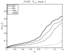
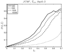
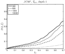
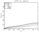
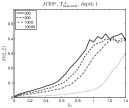
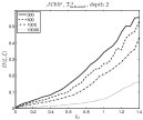
(a) $\mathtt{JC69}^{\ast}$

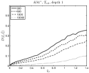
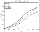
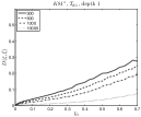
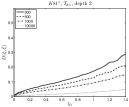
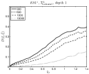
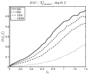
(b) $\mathtt{K81}^{\ast}$

Figure 3: Divergence $D(\xi,\hat{\xi})$ between the parameters, $\xi$, and their estimates, $\hat{\xi}$, calculated by Empar. Horizontal axis: original length of the inner branch.

Figure 3 depicts the results for $\mathtt{JC69}^{\ast}$ and $\mathtt{K81}^{\ast}$ on the three 4-taxon phylogenies, different alignment lengths and depths of the branches. The shapes of the distribution of $D$ for both models are very similar. As expected, the performance is weaker for long branches and short alignments. A great improvement is observed with the increase in the alignment length, e.g. $10,000nt$ depicts very accurate estimates. The performance under the $\mathtt{JC69}^{\ast}$ model (Fig. 3a )is better than that of $\mathtt{K81}^{\ast}$ (Fig.3b) for shorter branch lengths.

Parameter dispersion

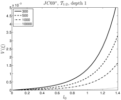
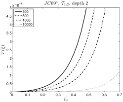
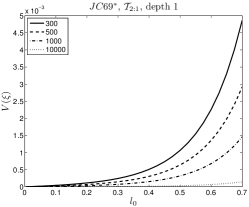
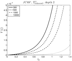
Figure 4: Distribution of variances of the estimated parameters for different alignment lengths and different lengths of the depth 1 (left) and depth 2 (right) branches under the $\mathtt{JC69}^{\ast}$ model: $\tau_{1:2}$ (top), $\tau_{2:1}$ (middle), $\tau_{\mathrm{balanced}}^{4}$ (bottom).

Figure 4 shows the variances of the estimated parameters for depth 1 and 2 branches on the $\tau_{\mathrm{balanced}}$, $\tau_{1:2}$, $\tau_{2:1}$ trees under the $\mathtt{JC69}^{\ast}$ model.

The variances show an exponential increase, which is most significant in the $\tau_{\mathrm{balanced}}^{4}$ tree for both depths, and the $\tau_{1:2}$ for depth 2. The results for the depth 1 branch in $\tau_{\mathrm{balanced}}$ and $\tau_{1:2}$ are very similar. The smallest variance was observed for the depth 2 of $\tau_{2:1}$. For alignments of length $10,000nt$ on four taxa we can say that the method is quite accurate (see also Tab.VI-VIII in the Supp. mat. C).

For the $\mathtt{K81}^{\ast}$ model we summarized the results on variances for each edge as the mean of combined variances of all samples (see formula (4)). The results are analogous to those of the $\mathtt{JC69}^{\ast}$ model, see Figure II in Supp. mat. C. As expected, the parameter estimates are less dispersed for shorter branches and longer alignments (see Tab. IX-XI in the Supp. mat. C).

Error in the branch lengths

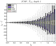
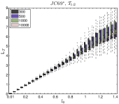
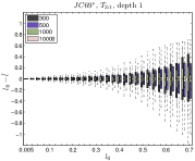
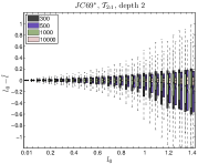
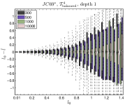
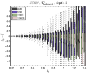
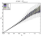
Figure 5: Error in the branch length estimation measured as the difference between the initial and the estimated branch lengths, $l_{0}-\hat{l}$, in the $1,000$ simulated data sets along the $\tau_{\mathrm{balanced}}^{4},\tau_{1:2},\tau_{2:1}$ trees under the $\mathtt{JC69}^{\ast}$ model (left and middle columns). Rightmost column displays the distribution of the estimated length of the tree, where $l_{0}$ labeling the horizontal axis corresponds to the length of the internal branch in $\tau$.

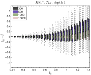
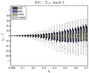
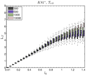
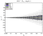
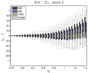
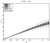
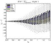
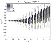
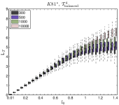
Figure 6: Error in the branch length estimation under the $\mathtt{K81}^{\ast}$ model (see Fig. 4 for details).

Using the formula (5) we calculated the actual difference $l_{0}-\hat{l}$ between the branch length $l_{0}$ computed from the original parameters $\xi$ and the branch length $\hat{l}$ computed using their MLEs $\hat{\xi^{e}}$. Negative values of this score imply overestimation of the branch length, while positive values indicate underestimation. The results are shown in Figures 5 and 6.

In the case of $\mathtt{JC69}^{\ast}$ we observe that the method presented here does not tend to underestimate or overestimate the lengths for the depth 1 branches in all the 4-taxon trees ($l_{0}-\hat{l}$ is centered at 0 (see Fig. 5). The depth 2 branches have a tendency towards overestimation of the length for branches longer than (approximately) $0.45$ for $\tau_{1:2}$, $0.9$ for $\tau_{2:1}$, and $0.8$ for the $\tau_{\mathrm{balanced}}^{4}$ trees. In the latter case, lengths longer than $1.2$ for alignments up to $1,000$nt show opposite trend of underestimating the true lengths. The values were accurate when the alignment lengths were increased in the case of $\tau_{1:2}$ and $\tau_{2:1}$. On the other hand, for $\tau_{\mathrm{balanced}}^{4}$ the alignments of $10,000$nt resulted in overestimation.

In the $\mathtt{K81}^{\ast}$ model the results are significantly more accurate (see Fig.  6). There is a trend of underestimation for branches longer than (approximately) $0.9$ for shorter alignments. That is especially noticeable for $\tau_{\mathrm{balanced}}^{4}$ and depth 1 branches of $\tau_{1:2}$. This trend diminishes with an increase in the alignment length. Overall, in the case of both models, the variance of the estimate is smaller for shorter lengths and both depth 1 and 2 branches of the $\tau_{2:1}$ tree.

In addition, we calculated the tree length $\mathsf{L}_{\tau}$ (i.e. the sum of its branch lengths) from the estimated parameters and compared it to the theoretical result on the original branch length $l_{0}$: $4.5l_{0}$ for $\tau_{1:2}$ (where $l_{0}$ is a depth 1 branch), $3l_{0}$ for $\tau_{2:1}$ ($l_{0}$ for depth 2 branch) and $5l_{0}$ for $\tau_{\mathrm{balanced}}^{4}$. The rightmost columns of Figures 5 and 6 show the results for 4-taxon trees for the $\mathtt{JC69}^{\ast}$ and $\mathtt{K81}^{\ast}$ models respectively. The length of the tree is estimated accurately for all trees, the estimates being best for $\tau_{2:1}$. The variance is small and decreasing with an increase in the data length. As the sequences get longer, the distribution is centered around the true value. This is especially visible for the $\mathtt{K81}^{\ast}$ model (see Fig.  6).

Results for larger trees

We run the analysis on the 6-taxon balanced tree, $\tau_{\mathrm{balanced}}^{6}$, under the $\mathtt{K81}^{\ast}$ model, for alignment lengths of $1,000$nt and $10,000$nt and branch length $\mathbf{l}\in\{0.01,0.1,0.3,0.5,0.7,0.9,1.1,1.3,1.4\}$. The $p-values$ of the corresponding tests confirm that the performance of the algorithm is very satisfactory (see Tab. XII in the Supp. mat. C). We have seen in the 4-taxon study that the tree with equal branch lengths gave worse results than the unbalanced trees. Thus, we expect the results of the depth 2 branches to be similarly challenged in this case.

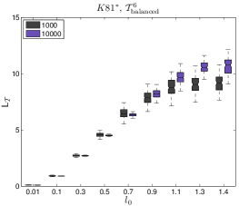
Figure 7: Estimated tree length as a function of the initial length of a branch of $\tau_{\mathrm{balanced}}^{6}$ ($\mathsf{L}_{\tau}=9l_{0}$) in $1,000$ data sets generated under the $\mathtt{K81}^{\ast}$ model.

Figure 7 depicts the estimated tree lengths. It can be seen that the estimates are accurate and the results improve for the alignments of $10,000$nt. As expected, the variance of the estimates increases with the increase in the length of the branch. By formula (5), long branches correspond to small values of the determinant of the transition matrix. Thus, statistical fluctuations in the parameter estimates have greater impact on the resulting length of the tree.

Next, we calculated the difference between the original and estimated branch lengths. In Figure 8a we see that the depth 1 branches show some degree of underestimation of the length for lengths $1.1-1.4$ and alignments of $1,000$nt. In the case of $10,000$nt, the results improve and can be expected to show little bias for even longer data sets. Branches of depth 2 show higher degree of underestimation with improvement for longer data sets. The divergence of the original and estimated parameters for transition matrices given by formula (7) is shown in Figure 8b. For branches of depth 1 and data of length $10,000$, the error is about 0.2. In the case of branches of depth 2, it is almost doubled for both alignment lengths. In both cases, branch lengths up to 0.5 give satisfactory results. The error of the estimates for longer branches seems to be approaching a plateau.

Combined variance of the estimated parameters is much decreased for the $10,000$nt data sets in comparison with the $1,000$nt, and is smaller for the depth 1 branch (see Fig. 8c ). Again, the exponential shape of the plot can be attributed to the logarithm appearing in the formula (5).

CONCLUSION

In order to evaluate the performance of the method proposed here under various circumstances, we conducted many tests on simulated data sets. We observed that the performance of Empar is most optimal for long alignments and short branch lengths.

It is worth noting that even for short alignments of 300nt or 500nt on 4 taxa, the estimated parameters approximate closely the original parameters in $\approx 95\%$ of the cases as proved by the normality test of the MLE. Moreover, the branch lengths calculated based on the parameters estimated by Empar were found very accurate already for short alignments. Though the measure of divergence $D$ for the parameters of transition matrices proposed here accumulates all errors in the entries of the transition matrix, alignment length of 10,000nt showed divergence values smaller than 0.1.

In this paper, we provide the first implementation of a tool for inferring continuous parameters under the discrete-time models. The method allows for accurate estimation of branch lengths in non-homogeneous data. There are two limitations to applicability of the method. Firstly, the algorithm has an exponential computational time increase with the number of taxa. This is a restriction due to the fact that the algorithm computes large matrices of dimension that is exponential in the total number of nodes of a tree. Running time of Empar on star trees with 3-8 nodes and equal branches of $0.5$ on Ubuntu 11.10, Intel Core i7 920 at 2.67 GHz with 6 Gb is given in Table 2. Secondly, the memory usage of Empar is approx. $8*4^{|N(\tau)|}$ and corresponds to the memory footprint of the matrix in the $\mathtt{EM}$ algorithm, e.g. for this matrix to fit in the memory of a 6Gb machine the bound on the number of nodes is $|N(\tau)|$ $\leq 14$.

Table 2: Empar performance time– estimating the parameters of $\mathtt{K81}^{\ast}$ on star trees with equal branch lengths of $0.5$, varying number of leaves, $L(\tau)$, for the MSAs of $1,000$ and $10,000nt$.

length $\mid$ n	3	4	5	6	7	8
1,000	0.004	0.02	0.033	0.222	1,049	7.14
10,000	0	0.011	0.043	0.171	1,044	6.95

We conclude that Empar is a highly reliable method for estimating branch lengths of relatively small number of taxa and trees with short branch lengths (e.g. closely related species), and achieves high accuracy even when the results are based on short sequences. In particular, Empar is a reliable method to compute quartets and to be used with quartet-based methods (see Berry et al. (1999) and Berry and Gascuel (2000)) on nonhomogeneous data.

FUNDING

Both authors were partially supported by Generalitat de Catalunya, 2009 SGR 1284. MC is partially supported by Ministerio de Educación y Ciencia MTM2009-14163-C02-02.We thank Roderic Guigó for generously providing funding for this project under grant BIO2011-26205 from the Ministerio de Educación y Ciencia (Spain).

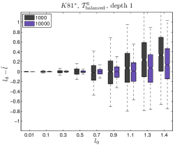
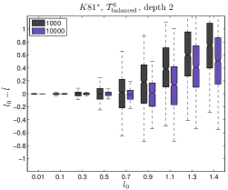
(a) Error in the branch length estimation for distinct depths of the branches.

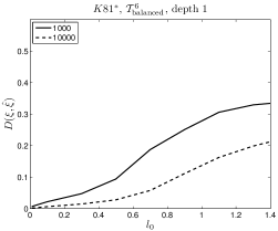
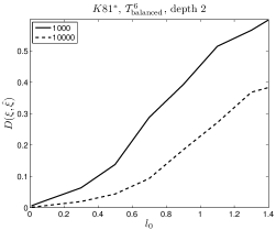
(b) The average $\mathsf{L}_{2}$ error between the original ($\xi$) and estimated ($\hat{\xi}$) parameters.

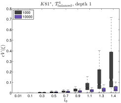
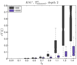
(c) Distribution of the combined variance for distinct depths of the branches.

Figure 8: Results for the $1,000$ data sets generated on the $\tau_{\mathrm{balanced}}^{6}$ tree for the $\mathtt{K81}^{\ast}$ model.

References

- Allman and Rhodes (2003) E S Allman and J A Rhodes. Phylogenetic invariants for the general Markov model of sequence mutation. Mathematical Biosciences, 186(2):113–144, 2003.
- Allman and Rhodes (2004) E S Allman and J A Rhodes. Mathematical Models in Biology. Cambridge University Press, January 2004. ISBN 0-521-52586-1.
- Allman and Rhodes (2007) E S Allman and J A Rhodes. Phylogenetic invariants. In O Gascuel and MA Steel, editors, Reconstructing Evolution. Oxford University Press, 2007.
- Ambroise (1998) C Ambroise. The EM Algorithm and Extensions , by G.M. McLachlan and T. Krishnan. Journal of Classification, 15(1):154–156, January 1998. ISSN 0176-4268.
- Barry and Hartigan (1987a) D Barry and J A Hartigan. Asynchronous distance between homologous DNA sequences. Biometrics, 43(2):261–276, 1987a. ISSN 0006-341X.
- Barry and Hartigan (1987b) D Barry and J A Hartigan. Statistical analysis of hominoid molecular evolution. Statistcal Sciences, 2(2):191–207, 1987b.
- Berry and Gascuel (2000) V Berry and O Gascuel. Inferring evolutionary trees with strong combinatorial evidence. Theoretical Computer Science, 240:271–298, 2000.
- Berry et al. (1999) V Berry, T Jiang, P Kearney, M Li, and T Wareham. Quartet cleaning: improved algorithms and simulations. In Proc. Europ. Symp. Algs. (ESA99), volume 1643 of LNCS, pages 313–324, 1999.
- Bruno and Halpern (1999) W J Bruno and A L Halpern. Topological bias and inconsistency of maximum likelihood using wrong models. Molecular Biology and Evolution, 16(4):564–566, 1999.
- Casanellas et al. (2011) M Casanellas, A M Kedzierska, and J Fernández-Sánchez. The space of phylogenetic mixtures of equivariant models. arXiv:0912.1957v1, 2011.
- Casanellas and Sullivant (2005) M Casanellas and S Sullivant. The strand symmetric model. In L Pachter and B Sturmfels, editors, Algebraic Statistics for computational biology, chapter 16. Cambridge University Press, 2005.
- Chang (1996) J T Chang. Full reconstruction of Markov models on evolutionary trees: identifiability and consistency. Math. Biosci., 137(1):51–73, 1996. ISSN 0025-5564.
- Dempster et al. (1977) A Dempster, N Laird, and D Rubin. Maximum likelihood estimation from incomplete data via the EM algorithm. Journal of the Royal Statistical Society, 39:1–38, 1977.
- Efron and Hinkley (1978) B Efron and D V Hinkley. Assessing the accuracy of the maximum likelihood estimator: Observed versus expected Fisher information. Biometrika, 65:457–483, 1978.
- Eo and DeWoody (2010) S H Eo and J A DeWoody. Evolutionary rates of mitochondrial genomes correspond to diversification rates and to contemporary species richness in birds and reptiles. Proc. Biol. Sci., 277:3587–92, Dec 2010.
- Felsenstein (1978) J Felsenstein. Cases in which parsimony or compatibility methods will be positively misleading. Systematic Biology, 27(4):401–410, 1978.
- Felsenstein (1993) J Felsenstein. PHYLIP– Phylogeny Inference Package (version 3.2). Cladistics, pages 164–166, 1993.
- Felsenstein (2004) J Felsenstein. Inferring Phylogenies. Sinauer Associates, Inc., 2004.
- Galtier and Gouy (1998) N Galtier and M Gouy. Inferring pattern and process: maximum likelihood implementation of a non-homogeneous model of DNA sequence evolution for phylogenetic analysis. Molecular Biology and Evolution, 154(4):871–879, 1998.
- Hartley (1958) H Hartley. Maximum likelihood estimation from incomplete data. Biometrics, 14:174–194, 1958.
- Hasegawa et al. (1985) M Hasegawa, H Kishino, and T Yano. Dating of the human-ape splitting by a molecular clock of mitochondrial DNA. J Molecular Biology, 22(2):160–174, 1985.
- Huelsenbeck and Hillis (1993) J. Huelsenbeck and D. Hillis. Success of phylogenetic methods in the four-taxon case. Systematic Biology, 42(2):247–264, 1993.
- Husmeier et al. (2005) D Husmeier, R Dybowski, and S Roberts. Probabilistic Modeling in Bioinformatics and Medical Informatics Advanced Information and Knowledge Processing. Springer Verlag, New York, 2005.
- Jayaswal et al. (2011) V Jayaswal, L S Jermiin, L Poladian, and J Robinson. Two stationary nonhomogeneous Markov models of nucleotide sequence evolution. Systematic Biology, 60(1):74–86, 2011.
- Jukes and Cantor (1969) T H Jukes and C R Cantor. Evolution of protein molecules. In H N Munro, editor, Mammalian Protein Metabolism, volume 3, pages 21–132. Academic Press, 1969.
- Kimura (1980) M Kimura. A simple method for estimating evolutionary rates of base substitutions through comparative studies of nucleotide sequences. Journal of Molecular Evolution, 16(2):111–120, 1980.
- Kimura (1981) M Kimura. Estimation of evolutionary distances between homologous nucleotide sequences. Proceedings of the National Academy of Sciences of the USA, 78(1):454–458, 1981.
- Lockhart et al. (1994) P J Lockhart, M A Steel, M D Hendy, and D Penny. Recovering evolutionary trees under a more realistic model of sequence evolution. Molecular Biology and Evolution, 11(4):605–612, 1994.
- Pachter and Sturmfels (2005) L Pachter and B Sturmfels, editors. Algebraic Statistics for computational biology. Cambridge University Press, November 2005. ISBN 0-521-85700-7.
- Rao (1973) C R Rao. Linear statistical inference and its applications. Wiley, New York, 1973.
- Ripplinger and Sullivan (2008) J Ripplinger and J Sullivan. Does choice in model selection affect maximum likelihood analysis? Systematic Biology, 57(1):76–85, 2008.
- Ripplinger and Sullivan (2010) J Ripplinger and J Sullivan. Assessment of Substitution Model Adequacy Using Frequentist and Bayesian Methods. Molecular Biology and Evolution, 27(12):2790–2803, 2010.
- Schwartz and Mueller (2010) R S Schwartz and R L Mueller. Branch length estimation and divergence dating: estimates of error in Bayesian and maximum likelihood frameworks. BMC Evolutionary Biology, 10(1):5, 2010.
- Semple and Steel (2003) C Semple and M Steel. Phylogenetics, volume 24 of Oxford Lecture Series in Mathematics and its Applications. Oxford University Press, Oxford, 2003. ISBN 0-19-850942-1.
- Steel et al. (1994) M A Steel, L A Székely, and M D Hendy. Reconstructing trees when sequence sites evolve at variable rates. Journal of Computational Biology, 1(2):153–163, 1994.
- Sullivan and Swofford (1997) J Sullivan and D L Swofford. Are guinea pigs rodents? the importance of adequate models in molecular phylogenetics. Journal of Mammalian Evolution, 4(2):77–86, 1997.
- Swofford (2003) D L Swofford. PAUP*. Phylogenetic Analysis Using Parsimony (*and Other Methods). Sinauer Associates, 2003. Version 4.
- Tanner (1996) M A Tanner. Tools for Statistical Inference: Methods for the Exploration of Posterior Distributions and Likelihood Functions, volume 3rd Edition. Springer Series in Statistics, New York: Springer, 1996.
- Tavaré (1986) S Tavaré. Some probabilistic and statistical problems in the analysis of DNA sequences. In Some mathematical questions in biology—DNA sequence analysis (New York, 1984), volume 17 of Lectures Math. Life Sci., pages 57–86. Amer. Math. Soc., Providence, RI, 1986.
- Wu (1983) C F J Wu. On the Convergence Properties of the EM Algorithm. Annals of Statistics, 11(1):95–103, 1983.
- Yang (1997) Z Yang. PAML: A program package for phylogenetic analysis by maximum likelihood. CABIOS, 15:555–556, 1997. URL http://abacus.gene.ucl.ac.uk/software/paml.html.
- Yang and Yoder (1999) Z Yang and A D Yoder. Estimation of the transition/transversion rate bias and species sampling. J. Mor. Evol., 48:274–283, 1999.
- Yap and Pachter (2004) V B Yap and L Pachter. Identification of evolutionary hotspots in the rodent genomes. Genome research, 14(4):574–9, April 2004.
- Zacks (1971) S Zacks. The theory of statistical inference. John Wiley and Sons, Inc., New York, 1971.
- Zou et al. (2011) L Zou, E Susko, Ch Field, and A J Roger. The Parameters of the Barry and Hartigan General Markov Model Are Statistically NonIdentifiable. Systematic Biology, 60:872–875, 2011.