On a problem of J. Nakagawa, K. Sakamoto, M. Yamamoto

Abstract

In this paper, we give a positive answer to a problem posed by Nakagawa, Sakamoto and Yamamoto concerning a nonlinear equation with a fractional derivative.

1 Introduction

In their overview paper concerning the mathematical analysis of fractional equations, Nakagawa, Sakamoto and Yamamoto [1] posed the problem concerning global solutions and blowing-up in a finite time of solutions to the equation

$$\left\{\begin{array}[]{cll}{}^{C}D_{0_{+}}^{\alpha}u(t)&=&-u(t)(1-u(t)),~{}~{}t>0,\\ u(0)&=&u_{0},\end{array}\right.$$ (1)

where ${}^{C}D_{0_{+}}^{\alpha}$ is the Caputo derivative defined for $g\in C^{1}[0,T]$ by

$${}^{C}D_{0_{+}}^{\alpha}g(t)=\frac{1}{\Gamma(1-\alpha)}\int_{0}^{t}(t-\tau)^{-\alpha}g^{\prime}(\tau)\,d\tau,$$

for $0<\alpha<1$.

Let us recall, in the case $\alpha=1$, the results concerning solutions of $(\ref{6})$ :

- For $0<u(0)<1$, the solution exists globally. Moreover,

$$|u(t)|\leq\frac{1}{e^{t}(1-u_{0})}\longrightarrow 0,\hbox{ as }{t\longrightarrow+\infty}.$$

- For $u(0)>1$, the solution can not exist globally.

Here, we show that the same conclusions are valid for equation $(\ref{6})$. Moreover we analyse :

1. The large time behavior of the global solution.
   

2. The blow-up time and profile of the blowing-up solutions.
   

Note that if we set $w=u-1$, then $(\ref{6})$ reads

$${}^{C}D_{0_{+}}^{\alpha}w(t)=w(t)(1+w(t)),$$

which describes the evolution of a certain species; the reaction term $w(1+w)$ describes the law of increase of the species.

2 Preliminaries

In this section, we present some definitions and results concerning fractional calculus that will be used in the sequel. For more information see [2].

The Riemann-Liouville fractional integral of order $0<\alpha<1$ of the integrable function $f:\mathbb{R}^{+}\longrightarrow\mathbb{R}$ is

$$J_{0_{+}}^{\alpha}f(t):=\frac{1}{\Gamma(\alpha)}\int_{0}^{t}(t-\tau)^{\alpha-1}f(\tau)\,d\tau,~{}~{}~{}t>0,$$

where $\Gamma(\alpha)$ is the Euler Gamma function.

The Riemann-Liouville fractional derivative of an absolutely continous function $f(t)$ of order $0<\alpha<1$ is

$$D_{0_{+}}^{\alpha}f(t):=\frac{1}{\Gamma(1-\alpha)}\frac{d}{dt}\int_{0}^{t}(t-\tau)^{-\alpha}f(\tau)\,d\tau.$$

The Caputo fractional derivative of an absolutely continous function $f(t)$ of order $0<\alpha<1$ is defined by

$${}^{C}D_{0_{+}}^{\alpha}f(t):=J_{0_{+}}^{1-\alpha}f^{\prime}(t)=\frac{1}{\Gamma(1-\alpha)}\int_{0}^{t}(t-\tau)^{-\alpha}f^{\prime}(\tau)\,d\tau.$$

Both derivatives present a drawback :

- The Riemann-Liouville derivative of a constant is different from zero,

$$D_{0_{+}}^{\alpha}C\neq 0,$$

while the Caputo derivative require $f^{\prime}(t)$ to calculate ${}^{C}D_{0_{+}}^{\alpha}f(t)$, for $0<\alpha<1$.

- We know that the Riemann-Liouville derivative of the Weierstrass function exists for any $0<\alpha<1$, but not for $\alpha=1$.

But for regular function with $f(0)=0$, both definitions coincide.

Next, we recall a lemma that will be used hereafter.

Lemma 2.1

( see [3]). Let $a,~{}b,~{}K,~{}\psi$ be non-negative continuous functions on the interval $I=(0,T)~{}~{}(0<T\leq\infty)$, let $\omega:(0,\infty)\longrightarrow\mathbb{R}$ be a continuous, non-negative and non-decreasing function with $\omega(0)=0$ and $\omega(u)>0$ for $u>0$, and let $A(t)=\max_{0\leq s\leq t}a(s)$ and $B(t)=\max_{0\leq s\leq t}b(s)$. Assume that

$$\psi(t)\leq a(t)+b(t)\int_{0}^{t}K(s)\omega(\psi(s))\,ds,~{}~{}t\in I.$$

Then

$$\psi(t)\leq H^{-1}\Big{[}H(A(t))+B(t)\int_{0}^{t}K(s)ds\Big{]},~{}~{}t\in(0,T_{1}),$$

where $H(v)=\int_{v_{0}}^{v}\frac{d\tau}{\omega(\tau)}~{}~{}(v\geq v_{0}>0)$, $H^{-1}$ is the inverse of $H$ and $T_{1}>0$ is such that $H(A(t))+B(t)\int_{0}^{t}K(s)ds\in D(H^{-1})$ for all $t\in(0,T_{1})$.

Here, we consider the problem

$$\left\{\begin{array}[]{cll}{}^{C}D_{0_{+}}^{\alpha}u(t)&=&-u(t)(1-u(t)),\\ u(0)&=&u_{0},\end{array}\right.$$ (2)

for $0<\alpha<1$ and $u_{0}>0$.

3 Main results

The local existence of solutions to $(\ref{P})$ is assured by the

Theorem 3.1

(see [2]). We consider the fractional differential equation of Caputo’s type given by

$$\left\{\begin{array}[]{cll}{}^{C}D_{0_{+}}^{\alpha}u(t)&=&f(t,u(t)),~{}~{}t>0,\\ u(0)&=&u_{0}.\end{array}\right.$$ (3)

For $0<\alpha<1$, $u_{0}\in\mathbb{R},~{}~{}b>0$ and $T>0$.
Assume that

1. $f\in C(R_{0},\mathbb{R})$ where $R_{0}=\{(t,u),~{}~{}0\leq t\leq T,~{}~{}|u-u_{0}|\leq b\}$ and $|f(t,u)|\leq M$ on $R_{0}$;

2. $|f(t,u)-f(t,v)|\leq L|u-v|,~{}~{}L>0,~{}~{}(t,u)\in R_{0}$.

Then there exists a unique solution $u\in C([0,h])$ for $(\ref{1})$, where $h=\min\Big{\{}T,\displaystyle\Big{(}\frac{b\Gamma(\alpha+1)}{M}\Big{)}^{\frac{1}{\alpha}}\Big{\}}$.

Theorem 3.2

Let $u$ be the solution of problem $(\ref{P})$. We have :

- If $~{}0<u_{0}<1$, the solution is global and it satisfies $~{}0<u<1$. Moreover, $u$ is given by

$$u(t)=E_{\alpha}(-t^{\alpha})u_{0}+\int_{0}^{t}(t-s)^{\alpha-1}E_{\alpha,\alpha}(-(t-s)^{\alpha})~{}u^{2}(s)ds,$$

and for some constants $c>0$ and $c_{1}>0$, we have

$$0<u(t)\leq\frac{1}{\frac{1}{cu_{0}}-\frac{c_{1}}{\alpha}t^{\alpha}},~{}~{}~{}~{}t>T_{0}:=\Big{(}\frac{\alpha}{c_{1}cu_{0}}\Big{)}^{\frac{1}{\alpha}}.$$

- If $~{}u_{0}>1$, the solution blows-up in a finite time $T^{*}$ : $\displaystyle\lim_{t\longrightarrow T^{*}}u(t)=+\infty$.
Moreover, we have the bilateral estimate :

$$\overline{w}(t)+1\leq u(t)\leq\widetilde{w}(t)+1,$$

and

$$\Big{(}\frac{\Gamma(\alpha+1)}{4(u_{0}-\frac{1}{2})}\Big{)}^{\frac{1}{\alpha}}\leq T^{*}\leq\Big{(}\frac{\Gamma(\alpha+1)}{u_{0}-1}\Big{)}^{\frac{1}{\alpha}},$$

where

$$\widetilde{w}(t)+\frac{1}{2}\sim\frac{\Gamma(2\alpha)}{\Gamma(\alpha)}(T_{\widetilde{w}}-t)^{-\alpha},\hbox{~{}~{}as}~{}~{}t\longrightarrow T_{\widetilde{w}},$$

$$\overline{w}(t)\sim\frac{\Gamma(2\alpha)}{\Gamma(\alpha)}(T_{\overline{w}}-t)^{-\alpha},\hbox{~{}~{}as}~{}~{}t\longrightarrow T_{\overline{w}}.$$

Here, $T_{\widetilde{w}}$ is the blow-up time of $~{}\widetilde{w}$, which satisfies

$$\Big{(}\frac{\Gamma(\alpha+1)}{4(u_{0}-\frac{1}{2})}\Big{)}^{\frac{1}{\alpha}}\leq T_{\widetilde{w}}\leq\Big{(}\frac{\Gamma(\alpha+1)}{u_{0}-\frac{1}{2}}\Big{)}^{\frac{1}{\alpha}},$$

and $T_{\overline{w}}$ is the blow-up time of $~{}\overline{w}$, which satisfies

$$\Big{(}\frac{\Gamma(\alpha+1)}{4(u_{0}-1)}\Big{)}^{\frac{1}{\alpha}}\leq T_{\overline{w}}\leq\Big{(}\frac{\Gamma(\alpha+1)}{u_{0}-1}\Big{)}^{\frac{1}{\alpha}}.$$

Proof of Theorem 3.2.

Part 1. If $0<u_{0}<1$, then the solution is global.
The solution to $(\ref{P})$ is given by

$$u(t)=E_{\alpha}(-t^{\alpha})u_{0}+\int_{0}^{t}(t-s)^{\alpha-1}E_{\alpha,\alpha}(-(t-s)^{\alpha})~{}u^{2}(s)ds.$$ (4)

Where the Mittag-Leffler functions $E_{\alpha}(-t^{\alpha})$ and $E_{\alpha,\alpha}(-t^{\alpha})$ are defined by :

$$E_{\alpha}(-t^{\alpha})=\sum_{j=0}^{\infty}\frac{(-1)^{j}t^{\alpha j}}{\Gamma(\alpha j+1)},$$

$$E_{\alpha,\alpha}(-t^{\alpha})=\sum_{j=0}^{\infty}\frac{(-1)^{j}t^{\alpha j}}{\Gamma(\alpha j+\alpha)}.$$

If $u_{0}>0$, then $u(t)>0$ as $E_{\alpha}(-t^{\alpha})>0$ and $E_{\alpha,\alpha}(-t^{\alpha})>0$.

Now, we set the function $\overline{u}(t)=1,~{}~{}t>0$.

As $0<u_{0}<1$, then $u_{0}<\overline{u}(0).$ In addition, we have

$${}^{C}D_{0_{+}}^{\alpha}\overline{u}(t)=0=-\overline{u}(t)(1-\overline{u}(t)).$$

Hence $\overline{u}$ is an upper solution of the equation $(\ref{P})$, and we have $u(t)<\overline{u}(t)=1$, (see [4], Thm. 2.4.3, p. 32).

Now, we examine the large time behavior of the global solution $0<u<1$.
For, let us recall the estimates ( see [5]) :
- For $0<\alpha<1$, there exists a constant $c>0$ such that,

$$0<E_{\alpha}(-t^{\alpha})\leq\frac{c}{1+t^{\alpha}}\leq c,~{}~{}~{}~{}t>0.$$ (5)

- For $0<\alpha<1$, there exists a constant $c_{1}>0$ such that

$$0<t^{\alpha-1}E_{\alpha,\alpha}(-t^{\alpha})\leq c_{1}t^{\alpha-1},~{}~{}~{}~{}t>0.$$ (6)

From $(\ref{3})$ and using the inequalities $(\ref{9})$ and $(\ref{10})$, we obtain

$$u(t)\leq cu_{0}+c_{1}\int_{0}^{t}(t-s)^{\alpha-1}u^{2}(s)ds.$$ (7)

We apply Lemma 2.1 to $(\ref{11})$ with $\omega(x)=x^{2},~{}K(s)=(t-s)^{\alpha-1},~{}A(t)=cu_{0},~{}B(t)=c_{1}.$
For $t>T_{0}$, we have

$$H(cu_{0})+\frac{c_{1}}{\alpha}t^{\alpha}\in D(H^{-1}),$$

where $\displaystyle H(v)=\frac{1}{v_{0}}-\frac{1}{v}~{}$ and $~{}\displaystyle H^{-1}(z)=\frac{1}{\frac{1}{v_{0}}-z},~{}~{}z\neq\frac{1}{v_{0}}$.
So we obtain,

$$u(t)\leq H^{-1}\Big{[}H(cu_{0})+\frac{c_{1}}{\alpha}t^{\alpha}\Big{]}.$$

Therefore

$$u(t)\leq\frac{1}{\frac{1}{cu_{0}}-\frac{c_{1}}{\alpha}t^{\alpha}},~{}~{}t>T_{0}.$$

Part 2. If $u_{0}>1$, then the solution blows-up in a finite time.

1. We show that $u>1$. For, let us define the new unknown function $w=u-1$. The function $w$ satisfies

   $$\left\{\begin{array}[]{cll}{}^{C}D_{0_{+}}^{\alpha}w(t)&=&w(t)(1+w(t)),\\ w(0):=w_{0}&=&u_{0}-1.\end{array}\right.$$ (8)

   As $u_{0}>1$, then $w_{0}>0$. Moreover, we have ([2])

   $$w(t)=E_{\alpha}(t^{\alpha})w_{0}+\int_{0}^{t}(t-s)^{\alpha-1}E_{\alpha,\alpha}((t-s)^{\alpha})~{}w^{2}(s)ds.$$

   Therefore, $w>0$; hence $u>1$.
   

2. We prove that $u$ blows-up in a finite time.
   
   Since we have $w(t)=u(t)-1$, it is seen that if $u(t)\longrightarrow\infty$ as $t\longrightarrow T^{*}$, then $w(t)\longrightarrow\infty$ as $t\longrightarrow T^{*}$ and vice versa. That is $w$ and $u$ will have the same blow-up time.
   We now must examine the blow-up properties of $w$, the solution of problem $(\ref{4})$. These are obtained by comparing $w(t)$ with the solutions of the following problems :

   $$\left\{\begin{array}[]{cll}{}^{C}D_{0_{+}}^{\alpha}\overline{w}(t)&=&\overline{w}~{}^{2}(t),\\ \overline{w}(0)&=&w_{0},\end{array}\right.$$ (9)

   and

   $$\left\{\begin{array}[]{cll}{}^{C}D_{0_{+}}^{\alpha}\widetilde{w}(t)&=&(\widetilde{w}(t)+\frac{1}{2})^{2},\\ \widetilde{w}(0)&=&w_{0}.\end{array}\right.$$ (10)

   We see by comparaison ([4]) that

   $$\overline{w}(t)\leq w(t)\leq\widetilde{w}(t),~{}~{}0\leq t<\min\{T_{\overline{w}},T_{\widetilde{w}}\}.$$

   Following the paper of Kirk, Olmstead and Roberts [6], we may assert that the solution $\overline{w}$ ( resp. $\widetilde{w}$) blows-up in a finite time $T_{\overline{w}}$ ( resp. $T_{\widetilde{w}}$), such that

   $$\Big{(}\frac{\Gamma(\alpha+1)}{4w_{0}}\Big{)}^{\frac{1}{\alpha}}\leq T_{\overline{w}}\leq\Big{(}\frac{\Gamma(\alpha+1)}{w_{0}}\Big{)}^{\frac{1}{\alpha}},$$

   and

   $$\Big{(}\frac{\Gamma(\alpha+1)}{4(w_{0}+\frac{1}{2})}\Big{)}^{\frac{1}{\alpha}}\leq T_{\widetilde{w}}\leq\Big{(}\frac{\Gamma(\alpha+1)}{w_{0}+\frac{1}{2}}\Big{)}^{\frac{1}{\alpha}}.$$

   So we have the following estimates

   $$T_{\widetilde{w}}\leq T^{*}\leq T_{\overline{w}}.$$

   Whereupon

   $$\Big{(}\frac{\Gamma(\alpha+1)}{4(w_{0}+\frac{1}{2})}\Big{)}^{\frac{1}{\alpha}}\leq T^{*}\leq\Big{(}\frac{\Gamma(\alpha+1)}{w_{0}}\Big{)}^{\frac{1}{\alpha}}.$$

   $\hfill\Box$

4 Numerical implementation

In this section, we will approximate the solution $u$ given by $(\ref{3})$. For, we need a numerical approximation of the convolution integral; this can be obtained using the convolution quadrature method.

As it has been explained in [7], a convolution quadrature approximates the continuous convolution

$$\int_{0}^{t}K(t-s)f(s)\,ds,~{}~{}t>0,$$

by a discrete convolution with a step size $h>0$. Then

$$\int_{0}^{t_{n}}K(t_{n}-s)f(s)\,ds\sim\sum_{j=0}^{n}\omega_{n-j}f(t_{j}),$$

where $t_{j}=jh,~{}j=0,1,2,...,n$ and the convolution quadrature weights $\omega_{j}$ are determined from their generating power series as

$$\sum_{j=0}^{\infty}\omega_{j}\zeta^{j}=\mathcal{L}\Big{\{}K(t):\frac{\delta(\zeta)}{h}\Big{\}}.$$

Here $\mathcal{L}\{K(t):s\}$ is the Laplace transform of $K(t)$ and $\delta(\zeta)$ is the generating polynomial for a linear multistep method.

Let $u_{n}$ be the approximation of $u(t_{n})$ for $n\geq 0$. Using the convolution quadrature method we obtain

$$u_{n}=(1-\omega_{0})^{-1}\Big{[}E_{\alpha}(-t^{\alpha})u_{0}+\sum_{j=0}^{n-1}\omega_{n-j}u_{j}\Big{]},~{}~{}n=1,2,3....$$

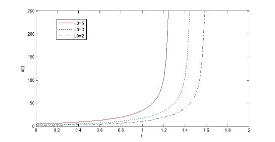
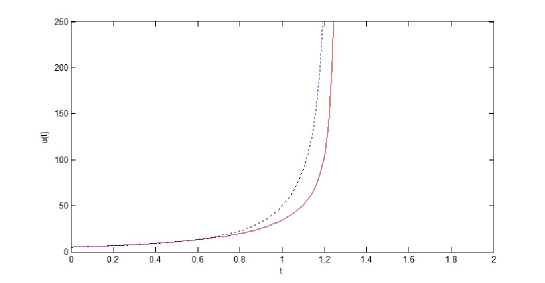
Figure 1: solutions for $\alpha=0.5$ and $u_{0}=5,~{}3,~{}2$.

Figure 2: solutions for $u_{0}=5$ and $\alpha=0.3,~{}0.5$.

Now, we introduce the following algorithm which gives the numerical approximation of solution to equation $(\ref{P})$.

Algorithm
Input : Give $\alpha$, $0<\alpha<1$ and $u_{0},~{}~{}u_{0}>1$.
Initializations : Discretize the time with a step size $h>0$; $t_{i}=ih$, for all $i=1,2,...,n$, $u^{1}_{appx}=u_{0},~{}~{}u^{1}=(u_{0})^{2}.$
Step 1 : Approximate the Mittag-Leffler function GML.
Step 2 : Calculate convolution quadrature weights W using the fast Fourier transform (FFT).
Step 3 : Calculate $u^{i}_{appx}$.
do

$\begin{array}[]{l}u^{i}=\textbf{GML}*u^{1}_{appx}+\textbf{W}*u^{i-1}.\\ u^{i}_{appx}=(1-\textbf{W}(1))^{-1}*u^{i}.\\ u^{i}=(u^{i}_{appx})^{2}.\\ i=i+1.\end{array}$
until ($u^{i}_{appx}$ blows up) or ($i>n$ ).
Output : Numerical approximation of $u$.

Example 1

For $Figure1$, we set $\alpha=0.5$; the initial conditions are respectively $u_{0}=5,~{}~{}u_{0}=3$ and $u_{0}=2$.
For $Figure2$, we take the initial condition $u_{0}=5$ and we plot the solutions; the dotted curve is the solution for $\alpha=0.3$ and the solid curve corresponds to the solution for $\alpha=0.5$.

As it has been proved, the solution blows up in a finite time which depends on $u_{0}$ and $\alpha$.

References

- [1] J. Nakagawa, K. Sakamoto and M. Yamamoto, Overview to mathematical analysis for fractional diffusion equations - new mathematical aspects motivated by industrial collaboration, Journal of Math-for-industry, Vol 2 (2010A-10), pp 99-108.
- [2] A. A. Kilbas, H. M. Srivastava and J. J. Trujillo, Theory and Applications of Fractional Differential Equations, Elsevier, 2006.
- [3] M. Kirane and N.-e. Tatar, Convergence Rates for a Reaction-Diffusion System, Journal for Analysis and Applications, Vol 20 (2001), No. 2, 347-357.
- [4] V. Lakshmikantham, S. Leela and J. Vasundhara Devi, Theory of Fractional Dynamic Systems, Cambridge Scientific Pub, Cambridge, UK (2009)
- [5] A. M. Krägeloh, Two families of functions related to the fractional powers of generators of strongly continuous contraction semigroups, J. Math. Anal. Appl. 283 (2003), 459-467.
- [6] C. M. Kirk, W. E. Olmstead and C. A. Roberts, A System of Nonlinear Volterra Equations with Blow-up Solutions, preprint.
- [7] M. Kirane and S. A. Malik, The profile of blowing-up solutions to a nonlinear system of fractional differential equations, Nonlinear Analysis 73 (2010), 3723-3736.