Quality Control System Response to Stochastic Growth of Amyloid Fibrils

Abstract

We introduce a stochastic model describing aggregation of misfolded proteins and degradation by the protein quality control system in a single cell. In analogy with existing literature, aggregates can grow, nucleate and fragment stochastically. We assume that the quality control system acts as an enzyme that can degrade aggregates at different stages of the growth process, with an efficiency that decreases with the size of the aggregate. We show how this stochastic dynamics, depending on the parameter choice, leads to two qualitatively different behaviors: a homeostatic state, where the quality control system is stable and aggregates of large sizes are not formed, and an oscillatory state, where the quality control system periodically breaks down, allowing for the formation of large aggregates. We discuss how these periodic breakdowns may constitute a mechanism for the sporadic development of neurodegenerative diseases. Key words: protein aggregation — Neurodegenerative diseases — stochastic dynamics — spiky oscillations — proteasome — lysosome

1 Introduction

Protein aggregation and formation of amyloid fibrils have been a subject of intense experimental and theoretical study in recent years. The main motivation has been that protein aggregation, including the formation of cytotoxic pre-amyloid species and larger inclusion bodies, seems to be the common theme underlying most known neurodegenerative diseases [1, 2]. Besides structural studies, several attempts have been made to build up coarse-grained models, able to characterise the aggregation process from a kinetic point of view without any influence of a cellular environment. One of the key features which are needed in the description is the existence of a nucleation mechanism [3]. During the late stages of the aggregation, the possibility of aggregates to break into smaller fragments also becomes important [4, 5]. Several other models have later been introduced, including more detailed mechanisms [6, 7, 8].

While amyloid growth and aggregation in vitro is quite well characterized nowadays, much less is known about the corresponding phenomenon in vivo. This is the main focus in this paper. The in vivo case is of crucial relevance since a common theme of many neurological disorders is undesired intercellular protein aggregation, and insights would be thus helpful to the understanding of disease development as well as treatments.

Apart from the experimental limitations, the in vivo case presents also a number of theoretical challenges. Accepting as a working hypothesis that the development of neurological disorders is directly associated with the aggregation process, it is unclear why such diseases develop in a time frame of several years, while in vitro aggregates can typically grow on timescales of hours or days. Another ubiquitous feature of neurological disorder is their sporadic development: degeneration is not gradual but occurs in almost-discrete steps. While a similar dynamical behaviour has been observed in vitro [9, 10], also in this case there is a large gap between the timescales observed in experiments and those characterizing the disease.

We examine the dynamics of in vivo aggregation where the cell’s quality control system tries to prevent protein aggregation by acting at different stages of the growth process. For example, in the case of Parkinson disease, it has been observed how $\alpha$-synuclein can be degraded both by the ubiquitin-proteasome system (UPS) and by autophagy [11]. The possibility of such mechanisms to degrade aggregates of $\alpha$-synuclein is currently under debate.

In a previous study, we explored the consequences of the interaction between $\alpha$-synuclein and the UPS system [12]. We found that such system displays a transition between a state in which the UPS system can effectively prevent aggregation, and one in which spiky oscillations are observed. During such spikes, the UPS is impaired, allowing for growth of aggregates. However, the model we considered lacked a description of the aggregation kinetics.

To address this issue, we study a model describing the behaviour of the battle between protein aggregation and the quality control system in a single cell. We implement the aggregation process in a similar way as in [7]: aggregates are formed when a nucleation threshold is passed, and grow according to the existing concentration of monomers. Further, large aggregates can break into smaller fragments. To this mechanism, we couple the response of the protein quality control system. We assume that its action can be modeled as an enzymatic degradation, whose efficiency depends on the size of the aggregate. We mostly identify this system with the UPS, as it is better characterized from a biochemical point of view than other systems such as lysosomes. However, larger fragments are more likely to be attacked by autophagy, whose possible effect we will also discuss.

In order to assess the effect of intrinsic noise on the resulting dynamics, we have implemented all reactions stochastically using the Gillespie algorithm [16]. We observe that, even in the presence of stochasticity, aggregation in this model is not continuous, but occurs in fairly regular spikes. During these spikes, aggregates of all sizes can quickly be formed. Such spikes become more irregular if the degrading agent is present on average in low numbers in the cell. Before discussing the consequences of our findings, we outline the details of our model.

2 Model

Our model describes the stochastic growth of fibrillar aggregates during constant attack by the cell’s protein quality-control system. We define $f_{n}$ as the number of free aggregates made up of $n$ monomers present in the cell, so that $f_{1}$ is the number of free monomers, or aggregation-prone proteins. We will assume that the action of the quality control system can be modelled as an enzymatic degradation, where we have the case of the UPS response system as an example in mind. The number of free degradation enzymes available in the cell is denoted by $E$. Such enzymes can degrade fibrils of size $n$ through the formation of a long lived complex $C_{n}$. The interplay between $f_{n},E$ and $C_{n}$ is summarised in Fig. (1) and discussed below.

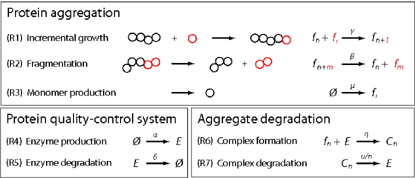
Figure 1: Total set of reactions that defines our model of protein aggregation (top panel) and subsequent degradation by the cell’s quality control system (bottom right panel). The quality-control system is under cellular regulation (bottom left panel).

In analogy with existing models [4, 7] we describe the dynamics of aggregate formation in terms of two basic processes (top panel in Fig. 1): (R1) step-wise growth by attachment of monomers to one of the fibril ends, and (R2) random breakage of aggregates into smaller fragments. Reactions (R1) and (R2) occur at rates $\gamma$ and $\beta$, respectively. In addition to (R1) there is a possibility to introduce a nucleation barrier so that the reaction in which two monomers bind (R1’) $f_{1}+f_{1}\xrightarrow{\gamma^{\prime}}f_{2}$ is slower than (R1), i.e. $\gamma^{\prime}\ll\gamma$. The dynamics of (R1) and (R2) have been shown to be consistent with results of in vitro aggregation experiments [7]. In addition to (R1) and (R2), we consider a constant production of monomers at rate $\mu$ (R3).

The cell’s protein quality-control system, here represented by a generic degradation enzyme $E$, attacks fibrillar aggregates of all sizes in order to keep their concentration at a low level. The enzyme is produced at rate $\alpha$ (R4) and each molecule is degraded with rate $\delta$ (R5) (bottom left panel). The steady-state concentration of $E$ in absence of fibrils is then $\alpha/\delta$.

The degradation of aggregates by the degradation enzyme is assumed to take place as a two-step process (bottom right panel). First, it binds to fibrils of a given size $n$ and forms a complex $C_{n}$ (R6). Then, in a time proportional to $n$, the aggregate is entirely degraded and the enzyme is released and ready to deal with another aggregate (R7). In general, it is unreasonable to assume that the degradation capability of the quality control is simply inversely proportional to $n$. A more realistic assumption would be to let $\eta$ and $\nu$ have a non-trivial size dependence. The functions $\eta(n)$ and $\nu(n)$ may be also different for different agents, describing the spectrum of aggregates that each of them can effectively bind and degrade. For example, a proteasome could be able to attack misfolded monomers and eventually early stage aggregates, while lysosomes might effectively attack larger bodies. However, given the poor biochemical characterisation of these agents, we consider only one of them at a time and keep $\eta$ and $\nu$ independent of $n$. However, to avoid the possibility of the enzyme to attack unreasonably large aggregates, we introduce an upper limit $n_{\rm max}$ to the aggregate size that the proteasome can bind to.

In summary, our model is defined by reactions (R1)-(R7) with ingoing parameters $\gamma$($\gamma^{\prime}$), $\beta$, $\mu$, $\alpha$, $\delta$, $\eta$, $\nu$ and $n_{\rm max}$.

3 Results

We investigated the dynamics of the model introduced in the previous section using computer simulations. In order to include properly the effects caused by intrinsic noise, we implemented all the reactions stochastichally via the Gillespie algorithm [16]. Parameters were selected according to physiological conditions based on measured aggregation rates of proteasomal dynamics. The one exception is $\alpha$ which is left as a free parameter in our model. Since we are interested in the long-time behaviour, all time units are in days. Reactions rates are therefore expressed in $[day]^{-1}$, $[day]^{-1}$ per molecule or $[day]^{-1}$ per couple of molecules, depending on reaction order (number of chemical species on the reaction’s left-hand side). We will start our analysis by identifying the enzyme with the ubiquitin-proteasome system, which we refer to simply as the proteasome, the main reason being that it is biochemically well characterised (compared to e.g. lysosomes).

The parameters characterizing the aggregating monomers have been chosen having $\alpha$-synuclein in mind as example. However, the model can be easily adapted to describe aggregation of other proteins. We fix the parameters according to this choice and later vary key parameters in order to probe the different behaviours of the model. The specific choice of all numerical values of the parameters is discussed in Appendix 6.

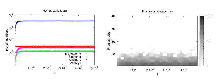
Figure 2: Homeostatic state. (left) Number of molecules as a function of time (right) size distribution of bound aggregates. The following parameters were used: $\gamma=2\cdot 10^{-5}$, $\gamma^{\prime}=2\cdot 10^{-10}$, $\beta=10^{-3}$, $n_{\rm max}=10^{6}$, $\mu=6\cdot 10^{4}$, $\alpha=10^{2}$, $\delta=0.1$, $\eta=0.02$, $\nu=10^{2}$. All rates are in unit $[day]^{-1}$, $[day]^{-1}$ per molecule or $[day]^{-1}$ per couple of molecules, depending on the order of the reaction.

Figure 2 shows the dynamics of the model with the parameter choice from Appendix 6 without any alteration. The result is a stationary homeostatic state, after a short period of transient behaviour from the initial conditions, where there is a chemical balance between proteasome concentration and the formation of aggregates. The proteasome is in the model denoted $E$ whereas filaments and bound filaments represent a sum over all sizes excluding the free monomers $f_{1}$, that is $\sum_{n>1}f_{n}$ and $\sum_{n}C_{n}$. The figure shows that their concentrations fluctuate moderately around well defined average values which means that the proteasome is fully functioning and keeps the total aggregate concentration down. In this homeostatic state there is also a fast decay (well fitted by an exponential) of the aggregate size distribution as a function of $n$ (right panel) as well as bound fibrils ($C_{n}$) (not shown).

Coupled kinetic equations for the aggregation process (R1)-(R2) with a finite pool of monomers were solved analytically in [7]. The model we consider here is more complicated due to the non-linear coupling with the proteasome and does therefore not lend itself easily to analytical treatments. The problem does however simplify if we let the aggregate size $n$ be a continuous variable. Indeed, one can show (see Appendix 7) that the aggregate size-distribution in the homeostatic case decays exponentially with $n$. This means that very large fibrillar aggregates are unlikely to be formed in this regime; as a consequence, the value of $n_{\rm max}$ is irrelevant, as soon as it is reasonably large. This contrasts the behaviour of the model in the absence of any proteasome degradation where fibrils grow at a much higher rate, up to a size which is essentially unlimited. An unlimited growth that in in vitro experiments becomes limited by the available pool of aggregating peptide chains [7].

Figure 3: Oscillatory state, number of molecules as a function of time. Parameters are same as Fig. 2 but $\mu$ is 5 times larger, $\mu=3\cdot 10^{5}$. (left) number of molecules as a function of time, (right) size distribution of bound aggregates.

If the monomer production rate ($\mu$) is increased, homeostasis breaks down and oscillations emerge (Fig. 3, left panel). In this regime there are dramatic drops in proteasome concentration which stays low for long periods of time, leading to a buildup of larger and larger fibrillar aggregates. The quality control system cannot in this case cope with the amount of aggregates present in the system which results in a non-exponential decay in the aggregate size distribution with $n$. The distribution becomes heavy tailed, and aggregates may reach sizes larger than $n_{\rm max}$, i.e. large enough to escape the repair system.

The striking outcome of the model is that destabilisation of the quality control system is episodic. The system alternates between states in which the quality control system is functioning, and short periods in which the proteasome is impaired. During such periods, aggregates of all sizes are predicted, as shown in the right panel of Fig. 3. This is a consequence of the fact that the growth dynamics, in the absence of the proteasome, is faster than the timescale of the recovery of the quality control system. The largest aggregates size that the proteasome can attack is controlled by $n_{\rm max}$ and if aggregates larger than $n_{\rm max}$ are formed, nothing can prevent such aggregates from reaching very large sizes, even when the quality control system has recovered. Finally, despite the fact that simulations are stochastic, the period of the oscillations is remarkably regular. This is a consequence of the (average) high copy number of all proteins involved.

We also remark that, starting from the homeostatic state of Fig. 2, the onset of oscillations can be triggered by varying different parameters. In particular, reducing the proteasome production rate $\alpha$, and/or the proteasome degradation efficiency $\nu$ trigger oscillations.

3.1 Lysosomal degradation

Autophagy is the process by which cytosolic membrane-bound compartments engulf substrates, such as mis-folded proteins or protein aggregates, that ultimately fuse with the lysosome for degradation of their content [19]. For example, mis-folded $\alpha$-synuclein protein in Parkinson’s disease has been identified as substrate for this type of autophagy [11]. Autophagy can be regarded as a back-up system to complement proteasomal degradation when it is overwhelmed or incapable of dealing with specific aggregated substrates. Indeed, experiments strongly suggest that the removal of mis-folded proteins through autophagy and the ubiquitin proteasome system are interconnected [20], as impairment of the ubiquitin proteasome system induces compensatory autophagy.

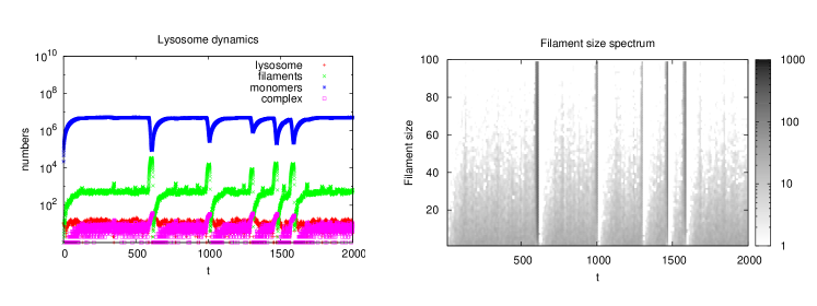
Figure 4: Oscillations in the presence of lysosome. Parameters are: $\gamma=2\cdot 10^{-5}$,$\gamma^{\prime}=2\cdot 10^{-10}$, $\beta=10^{-3}$, $n_{\rm max}=10^{6}$, $\mu=6\cdot 10^{4}$, $\alpha=1$,$\delta=0.1$, $\eta=0.02$, $\nu=10^{4}$. The only parameters that differ from the case of Fig. 2 are $\alpha$ and $\nu$. As usual, (left) number of molecules as a function of time, (right) size distribution of filaments. Notice how oscillations are much more stochastic as a consequence of the presence of small numbers of lysosomes.

This type of protein degradation is not so well characterised biochemically compared to for instance proteasomal degradation. But in order to test the effect of autophagic-like degradation we tuned our model parameters to represent the lysosome as an efficient enzyme present only in small copy numbers. We assumed a production rate $\alpha=1$ lysosome per day, and a degradation rate of $\delta=0.1$ lysosomes per day which corresponds to an average of $10$ lysosomes per cell at steady state. We assumed furthermore that the rate at which the enzyme degrades aggregates (per aggregate size) is $\nu=10^{4}$, which is a hundred times more efficient than the proteasome. Other mechanisms may be introduced to describe lysosomal dynamics in a more realistic ways. For example, one could introduce the possibility to deal with multiple aggregates at the same time, or a processing time having a different dependence on the $n$. For simplicity, we do not explore such possibilities here.

Figure 4 shows the results of a simulation for our new parameter choice. Even in this case we observe oscillations: the reason is that the higher efficiency is compensated by the lower numbers. The main difference between this case and that in fig. 3 is that the period of the oscillations is much more stochastic. This is a consequence of the enzyme being present in small numbers and the breakdown of the protein quality control system is much less regular in this case.

4 Discussion

In this paper we have studied the interplay between sequential growth of amyloid fibrils and its degradation by the quality control system in a single cell. Our model exhibit two types of dynamical behaviours. For one set of parameters the number of molecules is stationary and fluctuate around a well defined constant mean, while for the complementary set the system oscillates. These features were also captured in a simplified deterministic model [12] where the incremental fibrillar growth was replaced by a two-step process (small and large aggregates). However, the present study demonstrates how the dynamical behaviour observed in [12] is present also in a more mechanistic model, where the aggregation process is taken explicitly into account. Further, we demonstrate how such transition can occur for parameters values, to the best of our knowledge, under physiological conditions.

The main result of the model is that, in the regime in which the quality control system can not cope with the amount of fibrils, destabilisation of the homeostatic state gives rise to an oscillatory regime. Such oscillations are characterised by long time lapses in which the quality control system is functioning and prevents aggregation, separated by shorter lapses of time in which the quality control system is impaired and fibrils of large sizes can grow. The period of such oscillations depends on the parameter choice but is typically on the scale of months, thus predicting a slow and stepwise formation of large aggregates. Such phenomenology is reminiscent of the remarkably slow and sporadic development of neurodegenerative diseases.

Finally, we have shown that when the agent degrading the aggregates is present in large numbers, the resulting oscillations tend to be very regular and almost deterministic, while when the numbers are smaller oscillations are more stochastic.

There are clearly a number of generalisations one can consider to account for more accurate experimental evidences, such as the possibility of different interconnected repair systems, that attack aggregates at different stages of the growth process and with different efficiencies depending on the aggregate size. Our model should be considered as a minimal mechanistic model displaying such non-trivial phenomenology.

5 Acknowledgemens

This work was funded by the Danish National Research Foundation through the Center for Models of Life (CMOL). L.L acknowledges the financial support by the Knut and Alice Wallenberg foundation. D.E.O. is funded by the Danish Research Foundation (inSPIN) and the Lundbeck Foundation (BioNET 2).

6 Appendix: choice of parameters

In this appendix, we discuss our initial choice of parameters. We start the discussion with the parameters characterizing the aggregation/fragmentation part of the model. Studies on insulin [13] reported fibril growth rates around $0.3$ monomers per fibril per second in the presence of a monomer concentration of $0.17\ mM$. Similar studies on other molecules [14] report similar values. The average diameter of a dopaminergic neuron is from $10$ to $20\mu m$ (see e.g. [15]). This will give a cell volume around $v=10^{-11}l$. One single monomer in the cell will then correspond to a concentration of $1/(N_{A}v)\approx 2\cdot 10^{-13}M$ where $N_{A}$ is the Avogadro number. The growth rate per fibril per monomer will then be $0.25\cdot 10^{-9}s^{-1}$, that is approximately $2\cdot 10^{-5}$ monomers per fibril per day. In Ref. [13] it is estimated from reaction rate arguments that one every $10^{5}$ encounter events between filaments and monomer result in attachment.

Fitting models on aggregation to experiments suggest that the nucleation barrier can lead to an activation rate being $8$-$9$ orders of magnitudes smaller than the growth rate after nucleation [7]. This rate could however be different in vivo, since cell condition can significantly alter the nucleation barrier and favour/disfavour the formation of nucleation seeds. We choose a relatively high nucleation rate (compared with in vitro experiments), $\gamma^{\prime}=2\cdot 10^{-10}$.

We fixed a filament breakage rate $\beta=10^{-3}$ [7]. We observed that varying this rate has little effect on the outcome of the model, as most filaments are actively degraded by the quality control system. We also fixed $n_{\rm max}=10^{6}$; also this last parameter do not change the qualitative dynamics of the system when it is large enough, as the distribution of fibrils decays exponentially with their size in the stable regime. However, lowering the value will increase the chance that an aggregate may grow large enough to escape degradation to the quality control system. The production rate of monomers $\alpha$ is left as a free parameters. Since its value is typically large, to speed up the simulations we implemented an alternative reaction in which $100$ monomers at a time are produced with a rate $\alpha/100$. We checked in shorter simulations that such approximation does not alter significatively the results, thanks to the typical high numbers of monomers.

We move now to the parameters related to the proteasome. Proteasome lifetime is estimated to be 8-15 days in the cell [17, 18], leading to a degradation rate $\delta=0.1$. The proteasome production rate $\alpha$ is left as a free parameter. On general grounds, we may expect the proteasome to bind better to the filaments than to a monomer, leading to a complex formation $\eta$ being larger than $\gamma$. We pick $\eta=0.02$, corresponding to one successful binding event every $100$ encounters. A lower value of $\eta$ would make the proteasome less effective and would simply result in a higher threshold value for $\alpha$ to observe oscillations, without affecting the qualitative features of the model. Finally, the degradation rate of individual molecules by the proteasome is estimated to be on the order of minutes, so we pick $\nu=10^{3}$.

7 Appendix: continuous limit

If we treat the number of number of monomers $n$ forming an aggregate as a continuous variable, our model can be treated analytically. Adopting the notation from Fig. 1 the governing equations for the molecular concentrations are

$$\frac{\partial f_{n}(t)}{\partial t} = -\gamma\frac{\partial f_{n}(t)}{\partial n}-\eta f_{n}(t)E(t),$$ (1)

$$\frac{\partial C_{n}(t)}{\partial t} = \eta f_{n}(t)E(t)-\frac{\nu}{n}C_{n}(t),$$ (2)

$$\frac{\partial E(t)}{\partial t} = 1-E(t)+\int_{1}^{n_{\rm max}}dn\left(\eta f_{n}(t)E(t)-\frac{\nu}{n}C_{n}(t)\right),$$ (3)

Here we neglected filament breakage ($\beta=0$) and $n\geq 1$. We have also rescaled enzymatic growth and degradation rates as well as the filament length $n$ to 1. The constant production of monomers enters as the boundary condition

$$-\left(\frac{\partial f_{n}(t)}{\partial n}\right)_{n=1}=\mu.$$ (4)

In the homeostatic ”healthy” state it is straightforward to show that the time independent stationary (ST) concentrations are given by

$$f_{n}^{\rm ST}(n)=\frac{\mu\gamma}{\eta}e^{-\eta(n-1)/\gamma},\ \ \ \ C_{n}^{\rm ST}(n)=\frac{n\gamma\mu}{\mu}{\nu}e^{-\eta(n-1)/\gamma},\ \ \ \ P^{\rm ST}=1,$$ (5)

which shows that the size distribution of filaments $f_{n}^{\rm ST}$ decays exponentially. Moreover, the complex concentration $C_{n}^{\rm ST}$ grows with $n$ until it reaches a maximum at $\bar{n}=\eta/\gamma$ after which it also decays exponentially.

References

- 1. Ross C. A. and M. A. Poitier. 2004. Protein aggregation and neurodegenerative disease. Nature Medicine. 10:S10–S17.
- 2. Chiti F. and C. M Dobson. 2006. Protein misfolding, functional amyloid, and human disease. Annu. Rev. Biochem. 75:333–366.
- 3. Ferronejames F. A. and W. A. Eaton. 1985. Kinetics of Sickle Hemoglobin Polymerization II. A Double Nucleation Mechanism. Jour. Mol. Bio. 183:611–631.
- 4. Poschel T., N. V. Brilliantov and C. Frommel. 2003. Kinetics of Prion Growth. Biophys. Jour. 85:3460–3474.
- 5. Collins S. R., A. Douglass, R. D. Vale and J. S. Weissman. 2004. Mechanism of Prion Propagation: Amyloid Growth Occurs by Monomer Addition. Plos Biology 10:1582–1590.
- 6. Kunes K. C. , D. L. Cox and R. R. Singh. 2005. One-dimensional model of yeast prion aggregation. Phys Rev. E 72:051915.
- 7. Knowles T. P. J. et al. 2009. An analytical solution to the kinetics of breakable filament assembly. Science 326:1533.
- 8. Cabriolu R., D. Kashchiev and S. Auer. 2011. Size Distribution of Amyloid Nanofibrils. Biophys. Jour. 101:2232–2241.
- 9. Kellermayer M. S. Z. et al. 2008. Stepwise dynamics of epitaxially growing single amyloid fibrils. Proc. Natl. Acad. Sci. USA 105:141.
- 10. Fonslet J. et al. 2010. Stop-and-go kinetics in amyloid fibrillation. Physical Review E (Rapid Communications), 82:010901.
- 11. Webb J. L. et al. 2003. -Synuclein is degraded by both autophagy and the proteasome. Jour. Biol. Chem. 278:25009–25013.
- 12. Sneppen K., L. Lizana, M. H. Jensen, S. Pigolotti and D. Otzen. 2009. Modeling proteasome dynamics in Parkinson’s disease. Phys. Biol. 6:036005.
- 13. Knowles T. P. J. et al. 2007. Kinetics and thermodynamics of amyloid formation from direct measurements of fluctuations in fibril mass. Proc. Natl. Acad. Sci. 104:24.
- 14. Kusumoto Y., A. Lomakin, D. B. Teplow and G. B. Benedek. 1998. Temperature dependence of amyloid -protein fibrillization. Proc. Natl. Acad. Sci. 95:12277–12282.
- 15. Huot P., M. Levesque, A. Parent. 2007. The fate of striatal dopaminergic neurons in Parkinson’s disease and Huntington’s chorea. Brain. 130:222–232.
- 16. Gillespie D. T.. 1977. Exact stochastic simulation of coupled chemical reactions. J. Phys. Chem. 81:2340.
- 17. Tanaka K. and A. Ichihara. 1989. Half-life of proteasomes (multiprotease complexes) in rat liver. 1989. Biochem. Biophys. Res. Commun. 159:1309–1315.
- 18. Cuervo A. M., A. Palmer, A. J. Rivett, and E. Knecht. 1995. Degradation of proteasomes by lysosomes in rat liver. Eur. J. Biochem. 227:792–800.
- 19. Tyedmers J., A. Mogk and B. Bukau. 2010. Cellular strategies for controlling protein aggregation., Nature Reviews 11:777–788.
- 20. Pandey U. B. et al. 2007. HDAC6 rescues neurodegeneration and provides an essential link between autophagy and the UPS. Nature 447:860–864.