The Stochastic Gross–Pitaevskii Methodology

Abstract

We review the stochastic Gross–Pitaevskii approach for non-equilibrium finite temperature Bose gases, focussing on the formulation of Stoof; this method provides a unified description of condensed and thermal atoms, and can thus describe the physics of the critical fluctuation regime. We discuss simplifications of the full theory, which facilitate straightforward numerical implementation, and how the results of such stochastic simulations can be interpreted, including the procedure for extracting phase-coherent (‘condensate’) and density-coherent (‘quasi-condensate’) fractions. The power of this methodology is demonstrated by successful ab initio modelling of several recent atom chip experiments, with the important information contained in each individual realisation highlighted by analysing dark soliton decay within a phase-fluctuating condensate.
 
Unedited version of chapter to appear in
Quantum Gases: Finite Temperature and Non-Equilibrium Dynamics (Vol. 1 Cold Atoms Series).
N.P. Proukakis, S.A. Gardiner, M.J. Davis and M.H. Szymanska, eds.
Imperial College Press, London (in press).
See http://www.icpress.co.uk/physics/p817.html

I Introduction

Many theories have been devised to study the static and dynamic properties of weakly interacting, ultracold, atomic Bose gases at finite temperatures proukakis_jackson_08 ; blakie_bradley_08 . An important feature of these systems is that a condensate coexists with a non-condensed component beneath the temperature for the onset of Bose–Einstein condensation (BEC): repulsive interatomic interactions cause a depletion of atoms from the condensate, while thermal effects additionally promote atoms from the ground state of the system. An accurate description of partially condensed Bose gases thus requires a theory capable of describing condensed and non-condensed fractions within a unified framework. Symmetry breaking finite-temperature approaches rely on the explicit existence of a condensate mean field; such approaches are therefore useful away from the critical region, where there is a well-established condensate. Nonetheless, at temperatures close to the transition point, critical fluctuations make the definition of a condensate mean field much more difficult, an important consideration when studying condensate growth, or low dimensional geometries, for which the temperature range over which fluctuations are important is broader. Fluctuations play a key role in such cases and their presence motivates a stochastic description of the weakly interacting Bose gas. While several such methods are discussed in this book, this Chapter focuses on the non-equilibrium formulation of Stoof stoof_97 ; stoof_chapter_98 ; stoof_99 ; stoof_bijlsma_01 ; duine_stoof_01 , whose end result is a nonlinear Langevin equation for the field representing the condensate and its fluctuations.

II Methodology

To treat the fluctuations inherent to the process of Bose–Einstein condensation, a non-equilibrium probabilistic theory is required. Fokker–Planck equations, originally introduced to describe the Brownian motion of particles, achieve this by describing the time-evolution of an appropriate probability distribution. The mapping of a Fokker–Planck equation to an equivalent representation in terms of a Langevin equation, is often made for numerical impementation; such equations appear frequently in diverse fields including financial market modelling bouchaud_potters_book_00 , superconductors stephens_bettencourt_02 ; bustingorry_cugliandolo_06 , high-energy physics bettencourt_01 and turbulence rodean_book_96 .

II.1 Fokker–Planck Equation for an Ultracold Bose Gas

In Ref. stoof_99 , Stoof derived an equation for the evolution of the full probability distribution for the weakly-interacting Bose gas using a field-theoretic formulation of the non-equilibrium Keldysh theory danielewicz_84 , within the many-body T-matrix approximation. Using a Hartree–Fock-like ansatz, the total probability distribution was separated into a product of respective probability distributions for the condensate and thermal particles, which led to two coupled equations for these ‘subsystems’. Firstly, by integrating out the thermal degrees of freedom, the dynamics of the condensate distribution function, $P[\Phi^{*},\Phi;t]$, was found to obey:

$$i\hbar\frac{\partial{}}{\partial{t}}P[\Phi^{*},\Phi;t]=\\ \begin{aligned} &-\int d{\bf r}\ \frac{\delta}{\delta\Phi({\bf r})}\left(-\frac{\hbar^{2}}{2m}\nabla^{2}+V_{\rm ext}({\bf r})-iR({\bf r},t)+g|\Phi({\bf r},t)|^{2}-\mu(t)\right)\Phi({\bf r})P[\Phi^{*},\Phi;t]\\ &+\int d{\bf r}\ \frac{\delta}{\delta\Phi^{*}({\bf r})}\left(-\frac{\hbar^{2}}{2m}\nabla^{2}+V_{\rm ext}({\bf r})+iR({\bf r},t)+g|\Phi({\bf r},t)|^{2}-\mu(t)\right)\Phi^{*}({\bf r})P[\Phi^{*},\Phi;t]\end{aligned}\\ -\frac{1}{2}\int d{\bf r}\ \frac{\delta^{2}}{\delta\Phi({\bf r})\delta\Phi^{*}({\bf r})}\hbar\Sigma^{K}({\bf r};t)P[\Phi^{*},\Phi;t],$$ (1)

where, $\delta/\delta\Phi$ represents a functional derivative with respect to the complex field $\Phi$. The term $iR({\bf r},t)$ describes gain or loss of particles due to collisions which transfer atoms between the condensate and thermal cloud given by

$$R({\bf r},t)=2\pi g^{2}\int\frac{d{\bf p}_{2}}{(2\pi\hbar)^{3}}\int\frac{d{\bf p}_{3}}{(2\pi\hbar)^{3}}\int\frac{d{\bf p}_{4}}{(2\pi\hbar)^{3}}(2\pi\hbar)^{3}\ \delta({\bf p}_{2}-{\bf p}_{3}-{\bf p}_{4})\\ \times\delta(\varepsilon_{c}+\tilde{\varepsilon}_{2}-\tilde{\varepsilon}_{3}-\tilde{\varepsilon}_{4})\left[f_{2}(f_{3}+1)(f_{4}+1)-(f_{2}+1)f_{3}f_{4}\right],$$ (2)

where $\tilde{\varepsilon}_{i}=|{\bf p}_{i}|^{2}/2m+V_{\rm ext}({\bf r})+2g\langle|\Phi({\bf r},t)|^{2}\rangle$ is the Hartree–Fock energy of a thermal atom and $f_{i}\equiv f(\tilde{\varepsilon}_{i},t)$ the Wigner distribution function for thermal atoms.

The strength of the fluctuations is set by the Keldysh self-energy, defined by

$$\hbar\Sigma^{K}({\bf r},t)=-4\pi ig^{2}\int\frac{d{\bf p}_{2}}{(2\pi\hbar)^{3}}\int\frac{d{\bf p}_{3}}{(2\pi\hbar)^{3}}\int\frac{d{\bf p}_{4}}{(2\pi\hbar)^{3}}(2\pi\hbar)^{3}\ \delta({\bf p}_{2}-{\bf p}_{3}-{\bf p}_{4})\\ \times\delta(\varepsilon_{\rm c}+\tilde{\varepsilon}_{2}-\tilde{\varepsilon}_{3}-\tilde{\varepsilon}_{4})\left[f_{2}(f_{3}+1)(f_{4}+1)+(f_{2}+1)f_{3}f_{4}\right].$$ (3)

The $R$ term arises as the difference between the rate of scattering processes into and out of the low-lying modes of the system, $R=\hbar(\Gamma^{\rm out}-\Gamma^{\rm in})/2$, where $\Gamma^{\rm out}\propto f_{2}(f_{3}+1)(f_{4}+1)$ and $\Gamma^{\rm in}\propto(f_{2}+1)f_{3}f_{4}$, while the self-energy is the sum of these rates $\hbar\Sigma^{K}=-i\hbar(\Gamma^{\rm out}+\Gamma^{\rm in})$. Thus, although at equilibrium scattering processes should be zero on average ($\Gamma^{\rm out}\approx\Gamma^{\rm in}$), fluctuations nonetheless persist, highlighting the dynamical description of the equilibrium state.

The above Fokker–Planck equation for the condensate is coupled to a quantum Boltzmann equation for the distribution function describing the thermal cloud,

$$\frac{\partial{f}}{\partial t}+(\nabla_{\bf p}\tilde{\varepsilon})\cdot(\nabla f)-(\nabla\tilde{\varepsilon})\cdot(\nabla_{\bf p}f)=C_{12}[f]+C_{22}[f],$$ (4)

arising from the corresponding probability distribution evolution for thermal atoms. Scattering processes which transfer atoms between the condensate and thermal cloud are described by the collisional integral

$$C_{12}[f]=\frac{4\pi g^{2}}{\hbar}|\Phi|^{2}\int\frac{d{\bf p}_{2}}{(2\pi\hbar)^{3}}\int\frac{d{\bf p}_{3}}{(2\pi\hbar)^{3}}\int\frac{d{\bf p}_{4}}{(2\pi\hbar)^{3}}(2\pi\hbar)^{3}\ \delta({\bf p}_{2}-{\bf p}_{3}-{\bf p}_{4})\\ \times\delta(\varepsilon_{\rm c}+\tilde{\varepsilon}_{2}-\tilde{\varepsilon}_{3}-\tilde{\varepsilon}_{4})(2\pi\hbar)^{3}\ \left[\delta({\bf p}-{\bf p}_{2})-\delta({\bf p}-{\bf p}_{3})-\delta({\bf p}-{\bf p}_{4})\right]\\ \times[(f_{2}+1)f_{3}f_{4}-f_{2}(f_{3}+1)(f_{4}+1)],$$ (5)

while thermal-thermal collisions are represented by

$$C_{22}[f]=\frac{4\pi g^{2}}{\hbar}\int\frac{d{\bf p}_{2}}{(2\pi\hbar)^{3}}\int\frac{d{\bf p}_{3}}{(2\pi\hbar)^{3}}\int\frac{d{\bf p}_{4}}{(2\pi\hbar)^{3}}(2\pi\hbar)^{3}\ \delta({\bf p}+{\bf p}_{2}-{\bf p}_{3}-{\bf p}_{4})\\ \times\delta(\tilde{\varepsilon}+\tilde{\varepsilon}_{2}-\tilde{\varepsilon}_{3}-\tilde{\varepsilon}_{4})[(f+1)(f_{2}+1)f_{3}f_{4}-ff_{2}(f_{3}+1)(f_{4}+1)].$$ (6)

Thus, this formalism may be interpreted as a stochastic number-conserving generalisation of the ZNG kinetic theory zaremba_nikuni_99 ; griffin_nikuni_09 , which supplements dissipative processes affecting the condensate, by essential fluctuations.

II.2 Formulation as a Langevin Equation

The energy $\varepsilon_{\rm c}$ which appears in the expression for the self-energy and the damping term $iR({\bf r},t)$ is the energy associated with removing an atom from the condensate, which is given by the operator stoof_99 ; stoof_bijlsma_01 ; duine_stoof_01

$$\varepsilon_{\rm c}=-\frac{\hbar^{2}}{2m}\nabla^{2}+V_{\rm ext}({\bf r})+g|\Phi({\bf r},t)|^{2}.$$ (7)

As discussed by Duine and Stoof in Ref. duine_stoof_01 , the fact that $\varepsilon_{\rm c}$ is an operator dependent upon $\Phi$ leads to a complicated stochastic equation with multiplicative noise. To proceed, we may approximate the Wigner functions, $f({\bf r},{\bf p},t)$, by Bose–Einstein distributions, henceforth denoted by $n_{\rm BE}({\bf r},{\bf p})$. This assumption is consistent with an equilibrium thermal cloud, which we thus represent as a heat bath with a chemical potential, $\mu$, and temperature, $T$. This process leads to a relatively simple expression linking the damping term and the Keldysh self-energy stoof_99 ; duine_stoof_01 ,

$$-iR({\bf r},t)=\frac{1}{4}\hbar\Sigma^{K}({\bf r},t)\left[n_{\rm BE}(\varepsilon_{\rm c})+1/2\right]^{-1}.$$ (8)

A key observation is that this represents the fluctuation-dissipation relation for the system: it describes the relationship between the magnitude of fluctuations, set by $\hbar\Sigma^{K}({\bf r},t)$, and the damping due to the source term $iR({\bf r},t)$. This relation depends upon the equilibrium mode populations, set by the sum of thermal Bose–Einstein populations $n_{\rm BE}$, and an extra quantum contribution of half particle per mode, on average; physically, these respectively represent stimulated and spontaneous contributions to the scattering rate. As high energy atoms are here assumed to be close to thermal equilibrium, Eq. (8) should be valid in the regime of linear response, applicable to perturbations which do not strongly affect the thermal cloud.

The Fokker–Planck equation for the condensate, Eq. (1), can be mapped to an equivalent representation as a Langevin equation (see stoof_chapter_98 ), known in this context as the Stochastic Gross–Pitaevskii Equation (SGPE), which takes the form

$$i\hbar\frac{\partial{\Phi({\bf r},t)}}{\partial t}=\left[-\frac{\hbar^{2}}{2m}\nabla^{2}+V_{\rm ext}({\bf r})-iR({\bf r},t)+g|\Phi({\bf r},t)|^{2}-\mu\right]\Phi({\bf r},t)+\eta({\bf r},t).$$ (9)

This can be identified as a $T>0$ generalisation to the usual Gross–Pitaevskii Equation (GPE); it includes the scattering of particles into/out of the thermal cloud ($-iR\Phi$), with condensate fluctuations modelled via the dynamical noise term $\eta$. In order to obtain an equation that can be easily solved numerically, and upon noting that $\beta(\varepsilon_{\rm c}-\mu)$ is small at high $T$ ($\beta=1/k_{\rm B}T$), or close to equilibrium ($\varepsilon_{\rm c}\approx\mu$), we Taylor expand the Bose–Einstein distribution of Eq. (8) in terms of this variable. The result of retaining the leading order term in this expansion is to replace the fluctuation-dissipation relation of Eq. (8) with its classical counterpart, based upon the Rayleigh–Jeans distribution, yielding stoof_99 ; stoof_bijlsma_01 ; duine_stoof_01

$$-iR({\bf r},t)=\frac{\beta}{4}\hbar\Sigma^{K}({\bf r},t)\left(\varepsilon_{\rm c}-\mu\right).$$ (10)

Using Eq. (7) and Eq. (10) in Eq.(9) we finally obtain stoof_99 ; stoof_bijlsma_01 ; duine_stoof_01

$$i\hbar\frac{\partial{\Phi({\bf r},t)}}{\partial t}=\bigg{(}1+\frac{\beta}{4}\hbar\Sigma^{K}({\bf r},t)\bigg{)}\left[-\frac{\hbar^{2}}{2m}\nabla^{2}+V_{\rm ext}({\bf r})+g|\Phi({\bf r},t)|^{2}-\mu\right]\Phi({\bf r},t)+\eta({\bf r},t),$$ (11)

with Gaussian noise ensemble correlations $\langle\eta^{*}({\bf r},t)\eta({\bf r^{\prime}},t^{\prime})\rangle=i(\hbar^{2}/2)\Sigma^{K}({\bf r},t)\delta({\bf r}-{\bf r^{\prime}})\delta(t-t^{\prime})$. This is the form of the SGPE solved to date stoof_bijlsma_01 ; alkhawaja_andersen_02a ; proukakis_03 ; proukakis_schmiedmayer_06 ; proukakis_06b ; cockburn_proukakis_09 ; cockburn_nistazakis_10 ; cockburn_negretti_11 ; cockburn_gallucci_11 ; cockburn_nistazakis_11 . By analogy to other stochastic methods, $\Phi({\bf r},t)$ should now be understood as representing a unified description of atoms within the low-energy modes of the gas, up to some energy cutoff, that are in contact with a heat bath made up of the remaining higher energy thermal atoms.

II.3 Stochastic Hydrodynamics

The corresponding stochastic hydrodynamic theory led to the following generalisation of the usual continuity and Josephson equations duine_stoof_01 ,

$$\begin{split}\frac{\partial n_{c}({\bf r},t)}{\partial t}+\nabla\cdot\left(n_{c}({\bf r},t){\bf v}_{\rm s}({\bf r},t)\right)=&-\frac{\beta}{2}i\Sigma^{K}({\bf r},t)\left(\mu_{\rm c}({\bf r},t)-\mu\right)n_{c}({\bf r},t)\\ &+2\sqrt{n_{c}({\bf r},t)}\xi({\bf r},t),\end{split}$$ (12)

$$\hbar\frac{\partial\theta({\bf r},t)}{\partial t}-\frac{\beta}{4}i\hbar\Sigma^{K}({\bf r},t)\frac{\hbar^{2}\nabla\cdot\left(n_{c}({\bf r},t)\nabla\theta({\bf r},t)\right)}{2mn_{c}({\bf r},t)}=\mu-\mu_{\rm c}({\bf r},t)+\frac{\nu({\bf r},t)}{\sqrt{n_{c}({\bf r},t)}},$$ (13)

respectively, where $n_{c}$ and $\theta$ are the condensate density and phase, $\mu_{\rm c}({\bf r},t)=-(\hbar^{2}\nabla^{2}\sqrt{n_{c}({\bf r},t)}/2m\sqrt{n_{c}({\bf r},t)})+V_{\rm ext}({\bf r},t)+gn_{c}({\bf r},t)+(m/2){\bf v}^{2}_{s}({\bf r},t)$ and the velocity is given by the gradient of the phase ${\bf v}_{\rm s}({\bf r},t)={\hbar}\nabla\theta({\bf r},t)/m$. The noise terms are now given by $\langle\nu({\bf r},t)\nu({\bf r^{\prime}},t^{\prime})\rangle=i({\hbar^{2}}/{4})\hbar\Sigma^{K}({\bf r},t)\delta({\bf r}-{\bf r^{\prime}})\delta(t-t^{\prime})$ and $\langle\xi({\bf r},t)\xi({\bf r^{\prime}},t^{\prime})\rangle=i({\Sigma^{K}({\bf r},t)}/{4})\delta({\bf r}-{\bf r^{\prime}})\delta(t-t^{\prime})$. This approach is easily amenable to analytic variational methods duine_stoof_01 ; duine_leurs_04 .

II.4 Simple Numerical Implementation

The numerical solution of the SGPE, Eq. (11), is not much more complicated than the usual GPE: following Bijlsma and Stoof stoof_bijlsma_01 ; werner_drummond_97 , we seek to propagate the system from a time $t_{m}$ by a time step $\Delta t$, via

$$\Phi({\bf r},t_{m}+\Delta t)=\exp\left(-i[1+\beta\hbar\Sigma^{K}({\bf r})/4][\varepsilon_{\rm c}-\mu]\Delta t/\hbar\right)\left[\Phi({\bf r},t_{m})-\left(\frac{i}{\hbar}\right)\xi_{m}({\bf r})\right]$$ (14)

where we have defined the noisy field at the $m^{\rm th}$ time step as $\xi_{m}({\bf r})\equiv\exp\{-i[1+\beta\hbar\Sigma^{K}({\bf r})/4](\varepsilon_{\rm c}-\mu)t_{m}/\hbar\}\left\{\int_{t_{m}}^{t_{m}+\Delta t}dt^{\prime}\ \exp\{i[1+\beta\hbar\Sigma^{K}({\bf r})/4][\varepsilon_{\rm c}-\mu]t^{\prime}/\hbar\}\right\}\eta{({\bf r},t^{\prime})}$. This has correlations given by $\langle\xi_{m}^{*}({\bf r})\xi_{n}({\bf r^{\prime}})\rangle=i(\hbar^{2}/2)\Sigma^{K}({\bf r})\delta({\bf r}-{\bf r^{\prime}})\delta_{mn}\Delta t+\mathcal{O}(\Delta t^{2}).$ Making use of Cayley’s form for the exponential of Eq. (14), the problem is then reduced to the solution of

$$\left\{1+{i\left[1+\beta\hbar\Sigma^{K}({\bf r})/4\right]}\left(\varepsilon_{{\rm c},m+1/2}-\mu\right)\Delta t/{2\hbar}\right\}\Phi({\bf r},t_{m}+\Delta t)\\ =\left\{1-{i\left[1+\beta\hbar\Sigma^{K}({\bf r})/4\right]}\left(\varepsilon_{{\rm c},m+1/2}-\mu\right)\Delta t/{2\hbar}\right\}\left[\Phi({\bf r},t_{m})-\left(\frac{i}{\hbar}\right)\xi_{m}({\bf r})\right]$$ (15)

where $\varepsilon_{{\rm c},m+1/2}=\left[\varepsilon_{\rm c}(t_{m})+\varepsilon_{\rm c}(t_{m+1})\right]/2$ is the operator of Eq. (7) evaluated at the mid-point of the time step werner_drummond_97 ; the remaining step is to spatially discretise Eq. (15), which can be achieved using standard methods.

A typical simulation proceeds as follows: (i) Choose the necessary input parameters: $\mu$, $T$, atomic species, trapping potential; (ii) Create an ensemble of realisations, each corresponding to a unique set of noise realisations at each time step; (iii) Propagate this set of realisations to equilibrium, i.e. when observables (e.g. condensate number) become constant on average; equilibrium observables may be extracted by constructing correlation functions from the set of noise realisations, e.g. the density is given by $\langle\Phi^{*}\Phi\rangle\equiv\sum_{i=1}^{N}\Phi_{i}^{*}\Phi_{i}/N$ where $i$ denotes a particular noise realisation; (iv) Once at equilibrium, dynamical perturbations may also be studied, e.g. topological excitations (Section IV.2), or collective modes.

II.5 Interpretation: Single Runs and Extracting Coherence Properties

II.5.1 Single Versus Averaged Runs

By construction, physical properties are meant to be calculated by averaging over different realisations of the stochastic field $\Phi$. Nonetheless important information may also be extracted from single numerical runs; in this sense, the SGPE offers a strong analogy to experimental methods, in which data is obtained through repeated measurements from several independent experimental realisations. The SGPE was first applied in this way to demonstrate that important details of the growth and collapse dynamics of ⁷Li condensates gerton_strekalov_00 contained within single numerical realisations were lost by averaging over many runs duine_stoof_01 , suggesting that single stochastic numerical realisations are analogous to independent experimental realisations. The role of information extracted from single runs has been strengthened by further analysis, including spontaneous vortex formation via the Kibble–Zurek mechanism weiler_neely_08 , fluctuating soliton dynamics (Section IV.2) and in situ density fluctuations in atom chip experiments (Section IV.1).

II.5.2 A Posteriori Condensate/Quasi-Condensate Extraction

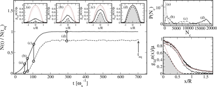
Figure 1: Left Plot: Growth of total (solid) and condensate number (dashed) during equilibration: insets show corresponding profiles at indicated times, with equilibrium results (at time $t_{\rm eq}$) shown by the thin solid and dotted lines. Right (Top): Condensate number distribution during growth at indicated times. (Bottom): Higher temperature data showing SGPE total (thick black noisy line) and quasi-condensate (thin black noisy) density profiles versus modified Popov total (thick grey lines) and quasi-condensate densities (dot-dashed grey). The SGPE Penrose–Onsager condensate (shaded region) is compared to the result of Eq. (16) (thin grey line). Figure adapted with permission from S.P. Cockburn et al., Comparison between microscopic methods for finite-temperature Bose gases, Phys. Rev. A, 83, 043619 (2011) cockburn_negretti_11 . Copyright (2011) by the American Physical Society.

The noisy wavefunction of the SGPE represents both coherent and incoherent atoms within low-energy modes in a unified manner, and a further statistical analysis is required to identify the coherent components. The density coherent quasi-condensate may be identified via $n_{\rm qc}(x)=\sqrt{2-g^{(2)}(x)}\,n(x)$ prokovev_ruebenacker_01 ; proukakis_06b ; bisset_davis_09 , where the second order correlation function $g^{(2)}(x)=\langle|\Phi(x)|^{4}\rangle/\langle|\Phi(x)|^{2}\rangle^{2}$. The additionally phase coherent fraction is associated to the Penrose–Onsager condensate mode penrose_onsager_56 , identified as the eigenmode corresponding to the largest eigenvalue of the system one-body density matrix $\rho(x,x^{\prime})\approx\langle\Phi^{*}(x)\Phi(x^{\prime})\rangle$ blakie_bradley_08 ; cockburn_negretti_11 ; wright_proukakis_11 ; this may be numerically obtained by diagonalising the density matrix — see Fig. 1 for an analysis of a $T>0$ 1d Bose gas based on this prescription. Motivated by Refs. alkhawaja_andersen_02a ; alkhawaja_andersen_02b , the Penrose–Onsager condensate of the SGPE is found to be well matched within a trapped system by the definition cockburn_negretti_11

$$n^{\prime}_{\rm c}(x)=g^{(1)}(0,x)\sqrt{2-g^{(2)}(x)}\,n(x),$$ (16)

where $g^{(1)}(0,x)=\rho(0,x)/\sqrt{n(0)n(x)}$ is the first order normalised correlation function. The dependence upon $g^{(1)}(0,x)$ illustrates clearly the additional phase coherence of the Penrose–Onsager condensate, relative to the quasi-condensate in which only density fluctuations are suppressed. Eq. (16) provides an alternative means of extracting the phase coherent fraction of a trapped gas from SGPE simulations, which accurately captures the condensate edge (but breaks down at very small distances from the trap centre); this method is also ideal for distinguishing between ‘condensate’ and ‘quasi-condensate’ in atom chip experiments cockburn_negretti_11 .

II.5.3 Comparison to the Modified Popov Method

As an independent validation of the above interpretation, Fig. 1 compares the SGPE result to the modified Popov theory of Stoof and co-workers andersen_alkhawaja_02 ; alkhawaja_andersen_02a ; alkhawaja_andersen_02b ; stoof_dickerscheid_book_09 , which accounts for contributions of phase fluctuations to all orders. Densities here are obtained within the local density approximation, via

$$n(x)=n_{\rm qc}(x)+\frac{1}{V}\sum_{{k}}\left\{\left[n_{\rm BE}(\epsilon_{{k}})+\frac{1}{2}\right]\frac{\varepsilon_{{k}}}{\epsilon_{{k}}}-\frac{1}{2}+\frac{g_{\rm 1d}n_{\rm qc}(x)}{2\varepsilon_{{k}}+2\mu}\right\},$$ (17)

with $n_{\rm qc}(x)=\left[\mu-V_{\rm ext}(x)-2g_{\rm 1d}n^{\prime}(x)\right]/g_{\rm 1d},$ where $\epsilon_{{k}}=[\varepsilon_{k}^{2}+2g_{\rm 1d}n_{\rm qc}\varepsilon_{k}]^{1/2}$ is the Bogoliubov dispersion relation, $\varepsilon_{k}=\hbar^{2}k^{2}/2m$, and $V$ is the system volume. Building on excellent agreement between the SGPE and modified Popov theory alkhawaja_andersen_02a , and the ideas introduced in alkhawaja_andersen_02b , the present comparison corroborates the above means of extracting the ‘true’ and quasi-condensate fractions of the gas from SGPE data. Thus, Eq. (16) is also expected to be a useful tool for analysing experimental density profiles. Further comparison between the SGPE and other one-dimensional Bose gases theories may be found in cockburn_negretti_11 .

III Validity Issues

III.1 Validity Domain

Two main assumptions underlie Eq. (11): Firstly, high energy thermal atoms within the system are treated as being at equilibrium (with their mean field contribution to $\Phi$ currently neglected). Thermal cloud dynamics — crucial when the thermal cloud is strongly perturbed — can be included by evolving the distribution functions via the quantum Boltzmann equation [Eq. (4)] stoof_99 .

Second is the so-called ‘classical approximation’: This terminology stems from the fact that the classical Rayleigh–Jeans distribution arises as the leading order term in a small $\beta(\varepsilon_{\rm c}-\mu)$ expansion of the Bose–Einstein distribution. While it does not constitute an essential ingredient of the theory, this approximation is very useful for numerical purposes, as it simplifies the scattering term $R({\bf r},t)$ to the form of Eq. (10), thus leading to the SGPE of Eq. (11) that is numerically solved. Although this is a well justified approximation for highly occupied (thus low energy) modes, it does lead to an ‘ultraviolet catastrophe’, which manifests through a dependence of physical observables upon the energy cutoff stoof_bijlsma_01 ; cockburn_proukakis_09 ; this problem is far more pronounced in spatial dimensions greater than one, due to the form of the density of states, and a possible solution is the introduction of divergence-cancelling counter-terms parisi_book_88 . The stochastic field $\Phi$ thus represents not just the phase-coherent part (condensate), but all atoms within modes up to an energy cutoff (in our simulations this is typically set by the spatial discretisation — see also Section IV.1).

III.2 Relevance to Other Theories

The SGPE is related to a number of theories discussed in this book: The closest link arises to the simple growth SPGPE gardiner_anglin_02 ; gardiner_davis_03 ; blakie_bradley_08 , which is very similar in nature, despite their rather distinct derivations. Various numerical differences arise in practice — most notably the use (or not) of a projector to separate low and high-lying modes. While this may be fundamentally important, the potential benefits from its use for dynamical predictions when low-lying modes are coupled to a static thermal cloud are not universally accepted — see Appendix C2 of Ref. proukakis_jackson_08 for a more detailed discussion of the links between these two approaches.

The SGPE is a grand canonical theory, as the exchange of particles and energy between the low-energy modes and heat bath is allowed. If, upon reaching equilibrium, $\hbar\Sigma^{K}$ is set to zero in both damping and noise terms (i.e. $iR=\eta=0$ in Eq. (11)), then it reduces to a multimode, finite temperature time-dependent GPE with a stochastically-sampled initial state. Such an approach, first applied by us to study quasi-condensate growth on an atom chip proukakis_schmiedmayer_06 , and subsequently used for finite temperature vortex dynamics rooney_bradley_10 , is similar in spirit (but not implementation proukakis_jackson_08 ) to the stochastic sampling of the Wigner distribution function evolved in truncated Wigner simulations steel_olsen_98 ; sinatra_lobo_02 ; norrie_thesis_05 .

Moreover, classical field methods for Bose gases levich_yakhot_78 ; svistunov_91 ; kagan_svistunov_97 ; marshall_new_99 ; goral_gajda_01a ; davis_morgan_01 , based upon the observation that the GPE accurately describes the dynamics of all highly occupied modes, typically start with a suitably random, multimode initial condition; this evolves to a classical equilibrium, sampling a microcanonical phase-space under ergodic GPE evolution marshall_new_99 ; goral_gajda_01a ; davis_morgan_01 ; connaughton_josserand_05 . Since $\mu$ and $T$ are input parameters for the SGPE, the latter approach may therefore be viewed as a more controlled way of generating a finite temperature initial state for classical field simulations cockburn_negretti_11 . However, one way in which the SGPE contrasts to ‘conventional’ classical field theories is through the generation of an ensemble of independent realisations, with physical observables (such as correlation functions) generated by ensemble averaging over many noise realisations (although see, for example, also sinatra_lobo_01 ). In classical field theories, such observables are instead typically generated by sampling the system at many different times, chosen so as to be sufficiently far apart.

By construction, the SGPE incorporates fluctuations into the condensate mean-field stochastically, whereas these can at most be a posteriori included in theories based on symmetry-breaking. Although we have focused here on numerical realisations with a static thermal cloud, the SGPE is in general intended to be coupled to a quantum Boltzmann equation for the thermal cloud; in this sense the full theory of Stoof may be considered as an (explicitly $U(1)$-symmetry-preserving) generalisation of the ZNG method zaremba_nikuni_99 ; griffin_nikuni_09 . The main importance of including fluctuations is for describing dynamical processes in the region of critical fluctuations (enhanced in low-dimensional systems), or for accounting for experimental shot-to-shot variations, whereas a ZNG-type approach could only account for averaged properties, albeit doing so very accurately. Finally, setting $\eta\rightarrow 0$ but maintaining the dissipative contribution to Eq. (11) leads to the commonly used Dissipative GPE (DGPE), with an ab initio expression for the damping rate, as opposed to phenomenological input.

IV Applications

IV.1 Comparison to Quasi-1d Bose Gas Experiments

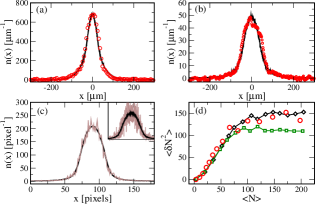
Figure 2: Quasi-1d SGPE model (solid black line) versus experimental density profiles (circles) from (a) Trebbia et al. trebbia_esteve_06 and (b) van Amerongen et al. vanamerongen_vanes_08 . (c) Main Plot: Single-run density, binned to experimental CCD camera resolution for the experiment of Armijo et al. armijo_jacqmin_10 (grey noisy) vs. average over 1000 realisations (black), with corresponding raw SGPE single-run data shown in the inset. (d) Density flutuations per binned average number predicted by the quasi-1d (black diamonds) and 1d (squares) SGPE [based on the binning procedure illustrated in (c)] versus experimental data of Armijo et al. (circles). Figure adapted with permission from S.P. Cockburn et al., Quantitative study of quasi-one-dimensional Bose gas experiments via the stochastic Gross–Pitaevskii equation, Phys. Rev. A 84, 023613 (2011) cockburn_gallucci_11 . Copyright (2011) by the American Physical Society.

Atom chips reichel_vuletic_book_11 facilitate controlled experiments with weakly-interacting, effectively one-dimensional Bose gases schumm_hofferberth_05 ; esteve_trebbia_06 ; trebbia_esteve_06 ; hofferberth_lesanovsky_06 ; jo_choi_07 ; jo_shin_07 ; hofferberth_lesanovsky_07 ; vanamerongen_vanes_08 ; hofferberth_lesanovsky_08 ; baumgartner_sewell_10 ; armijo_jacqmin_10 ; manz_bucker_10 ; armijo_jacqmin_11 , including in situ measurements, thus allowing for precision tests against theory. Importantly, fluctuations play a key role over a wide temperature regime for such extremely elongated geometries, thus making the SGPE a prime candidate for modelling such systems cockburn_gallucci_11 . Figure 2 shows a comparison between the SGPE and several, independent sets of quasi-1d experimental data. The agreement is excellent when comparing both density profiles [Fig.2(a)–(b)] and density fluctuations [Fig.2(d)]; the latter requires the binning of raw SGPE data [see Fig.2(c)] to bins of width set by the resolution in a given experiment, a key step required to achieve a consistent analysis of fluctuations. Experimentally, a system is considered as one-dimensional if $\mu,k_{\mathrm{B}}T\ll\hbar\omega_{\perp}$. If the first requirement is not satisfied, the replacement $g_{\rm 1d}|\psi|^{2}\rightarrow\hbar\omega_{\perp}[\sqrt{1+4a|\psi|^{2}}-1]$ fuchs_leyronas_03 ; gerbier_04 ; mateo_delgado_07 can account for the transverse swelling of the gas; in addition, if $k_{\mathrm{B}}T\not\ll\hbar\omega_{\perp}$, then we should also account for atoms in transverse excited modes which contribute a density $n_{\perp}(x)=({1}/{\lambda_{\rm dB}})\sum_{j=1}^{\infty}(j+1){\rm g}_{1/2}(e^{[\mu-V_{\rm ext}(x)-j\hbar\omega_{\perp}]/k_{\mathrm{B}}T})$ vanamerongen_vanes_08 (${\rm g}_{1/2}(\bullet)$: polylogarithm of order $1/2$). These two amendments yield a quasi-1d SGPE cockburn_gallucci_11 , which is cutoff independent (as both below and above cutoff physics is included in the model in an approximate, but self-consistent manner), and thus accurately models experiments in the crossover from one to three dimensions cockburn_gallucci_11 ; gallucci_cockburn_12 .

IV.2 Dark Soliton Dynamics in a Quasi-Condensate

As the equilibrium state of the SGPE agrees well with both experiment cockburn_gallucci_11 and alternative theories in suitable limits cockburn_negretti_11 , it constitutes an ideal ab initio approach for finite temperature Bose gas dynamics proukakis_schmiedmayer_06 ; cockburn_nistazakis_10 ; cockburn_thesis_10 ; cockburn_nistazakis_11 (see also proukakis_03 ; bradley_gardiner_08 ; weiler_neely_08 ; damski_zurek_10 ; rooney_bradley_10 ). This is particularly true for perturbations which do not push the thermal cloud far from equilibrium, making the dynamics of a dark soliton a perfect candidate. Including fluctuations in the background field leads to ‘shot-to-shot’ variations in soliton behaviour, as evident from indicative trajectories shown in Fig. 3(b). The corresponding histogram of decay times over the ensemble of realisations (Fig. 3(a)) is well-fitted by a lognormal distribution, displaying an extended tail at long times, indicative of very long-lived solitons, relative to the average soliton decay time cockburn_nistazakis_10 ; cockburn_thesis_10 ; cockburn_nistazakis_11 , consistent with experiments becker_stellmer_08 . These distributions are shown for a range of temperatures in Fig. 3(c) (inset), with the average times found to vary with temperature as $\langle\tau\rangle\sim T^{-4}$ (main plot). The distribution of soliton decay times obtained via the SGPE, relative to the single mean field DGPE result, indicates that consideration of many realisations of the stochastic wavefunction allows one to construct a representation of the full probability distribution for the gas; moreover, our analysis highlights once more the important feature that useful information is also retained within individual SGPE runs, which thus bear strong similarities to single-shot experimental realisations duine_stoof_01 ; weiler_neely_08 ; cockburn_nistazakis_10 ; cockburn_thesis_10 ; cockburn_gallucci_11 ; cockburn_nistazakis_11 .

Figure 3: (a) Histogram of soliton decay times and (b) example SGPE soliton trajectories at $T=175$nK, from the indicated bins, shown by vertical dot-dashed, solid and dashed black lines; the solid grey trajectory corresponds to the DGPE result. (c) Average decay times extracted from soliton decay time histograms at several temperatures, the fits to which are shown in the inset. Subplots adapted with permission from S.P. Cockburn et al., Matter-Wave Dark Solitons: Stochastic versus Analytical Results, Phys. Rev. Lett. 104, 174101 (2010) cockburn_nistazakis_10 and S.P. Cockburn et al., Fluctuating and dissipative dynamics of dark solitons in quasi-condensates, Phys. Rev. A 84, 043640 (2011) cockburn_nistazakis_11 . Copyright (2010) and (2011) by the American Physical Society.

References

- (1) N. P. Proukakis and B. Jackson, J. Phys. B 41, 203002 (2008)
- (2) P. B. Blakie, A. S. Bradley, M. J. Davis, R. J. Ballagh, and C. W. Gardiner, Adv. Phys. 57, 363 (2008)
- (3) H. T. C. Stoof, Phys. Rev. Lett. 78, 768 (1997)
- (4) H. T. C. Stoof, in Dynamics: Models and Kinetic Methods for Non-equilibrium Many Body Systems, NATO ASI Proceedings, Vol. 317, edited by J. Karkheck (Kluwer, Dordrecht, 2000) pp. 491–502, arXiv:cond-mat/9812424
- (5) H. T. C. Stoof, J. Low Temp. Phys. 114, 11 (1999)
- (6) H. T. C. Stoof and M. J. Bijlsma, J. Low Temp. Phys. 124, 431 (2001)
- (7) R. A. Duine and H. T. C. Stoof, Phys. Rev. A 65, 013603 (2001)
- (8) J. P. Bouchaud and M. Potters, Theory of Financial Risks (Cambridge University Press, Cambridge, 2000)
- (9) G. J. Stephens, L. M. A. Bettencourt, and W. H. Zurek, Phys. Rev. Lett. 88, 137004 (2002)
- (10) S. Bustingorry, L. F. Cugliandolo, and D. Domínguez, Phys. Rev. Lett. 96, 027001 (2006)
- (11) L. M. A. Bettencourt, Phys. Rev. D 63, 045020 (2001)
- (12) H. C. Rodean, Stochastic Lagrangian models of turbulent diffusion (American Meteorological Society, Boston, Mass., 1996)
- (13) P. Danielewicz, Annals of Physics 152, 239 (1984)
- (14) E. Zaremba, T. Nikuni, and A. Griffin, J. Low Temp. Phys. 116, 277 (1999)
- (15) A. Griffin, T. Nikuni, and E. Zaremba, Bose-Condensed Gases at Finite Temperatures (Cambridge University Press, Cambridge, 2009)
- (16) U. A. Khawaja, J. O. Andersen, N. P. Proukakis, and H. T. C. Stoof, Phys. Rev. A 66, 013615 (2002)
- (17) N. P. Proukakis, Las. Phys. 13, 527 (2003)
- (18) N. P. Proukakis, J. Schmiedmayer, and H. T. C. Stoof, Phys. Rev. A 73, 053603 (2006)
- (19) N. P. Proukakis, Phys. Rev. A 74, 053617 (2006)
- (20) S. P. Cockburn and N. P. Proukakis, Las. Phys. 19, 558 (2009)
- (21) S. P. Cockburn, H. E. Nistazakis, T. P. Horikis, P. G. Kevrekidis, N. P. Proukakis, and D. J. Frantzeskakis, Phys. Rev. Lett. 104, 174101 (2010)
- (22) S. P. Cockburn, A. Negretti, N. P. Proukakis, and C. Henkel, Phys. Rev. A 83, 043619 (2011)
- (23) S. P. Cockburn, D. Gallucci, and N. P. Proukakis, arXiv:1103.2740(2011)
- (24) S. P. Cockburn, H. E. Nistazakis, T. P. Horikis, P. G. Kevrekidis, N. P. Proukakis, and D. J. Frantzeskakis, arXiv:1107.3855(2011)
- (25) R. A. Duine, B. W. A. Leurs, and H. T. C. Stoof, Phys. Rev. A 69, 053623 (2004)
- (26) M. J. Werner and P. D. Drummond, Journal of Computational Physics 132, 312 (1997)
- (27) J. M. Gerton, D. Strekalov, I. Prodan, and R. G. Hulet, Nature 408, 692 (2000)
- (28) C. N. Weiler, T. W. Neely, D. R. Scherer, A. S. Bradley, M. J. Davis, and B. P. Anderson, Nature 455, 948 (2008)
- (29) N. Prokof’ev, O. Ruebenacker, and B. Svistunov, Phys. Rev. Lett. 87, 270402 (2001)
- (30) R. N. Bisset, M. J. Davis, T. P. Simula, and P. B. Blakie, Phys. Rev. A 79, 033626 (2009)
- (31) O. Penrose and L. Onsager, Phys. Rev. 104, 576 (1956)
- (32) T. M. Wright, N. P. Proukakis, and M. J. Davis, Phys. Rev. A 84, 023608 (2011)
- (33) U. Al Khawaja, J. O. Andersen, N. P. Proukakis, and H. T. C. Stoof, Phys. Rev. A 66, 059902(E) (2002)
- (34) J. Andersen, U. A. Khawaja, and H. Stoof, Phys. Rev. Lett. 88, 070407 (2002)
- (35) H. T. C. Stoof, D. B. M. Dickerscheid, and K. Gubbels, Ultracold Quantum Fields, Theoretical and Mathematical Physics (Springer, 2009)
- (36) G. Parisi, Statistical Field Theory (Addison-Wesley, Redwood City, Calif., 1988)
- (37) C. W. Gardiner, J. R. Anglin, and T. I. A. Fudge, J. Phys. B 35, 1555 (2002)
- (38) C. W. Gardiner and M. J. Davis, J. Phys. B 36, 4731 (2003)
- (39) S. J. Rooney, A. S. Bradley, and P. B. Blakie, Phys. Rev. A 81, 023630 (2010)
- (40) M. J. Steel, M. K. Olsen, L. I. Plimak, P. D. Drummond, S. M. Tan, M. J. Collett, D. F. Walls, and R. Graham, Phys. Rev. A 58, 4824 (1998)
- (41) A. Sinatra, C. Lobo, and Y. Castin, J. Phys. B 35, 3599 (2002)
- (42) A. A. Norrie, A Classical Field Treatment of Colliding Bose-Einstein Condensates, Ph.D. Thesis (University of Otago, Dunedin, 2005)
- (43) E. Levich and V. Yakhot, Journal of Physics A: Mathematical and General 11, 2237 (1978)
- (44) B. Svistunov, J. Moscow Phys. Soc. 1, 373 (1991)
- (45) Y. Kagan and B. V. Svistunov, Phys. Rev. Lett. 79, 3331 (1997)
- (46) R. J. Marshall, G. H. C. New, K. Burnett, and S. Choi, Phys. Rev. A 59, 2085 (1999)
- (47) K. Goral, M. Gajda, and K. M. Rzazewski, Optics Express 8, 92 (2001)
- (48) M. J. Davis, S. A. Morgan, and K. Burnett, Phys. Rev. Lett. 87, 160402 (2001)
- (49) C. Connaughton, C. Josserand, A. Picozzi, Y. Pomeau, and S. Rica, Phys. Rev. Lett. 95, 263901 (2005)
- (50) A. Sinatra, C. Lobo, and Y. Castin, Phys. Rev. Lett. 87, 210404 (2001)
- (51) J.-B. Trebbia, J. Esteve, C. I. Westbrook, and I. Bouchoule, Phys. Rev. Lett. 97, 250403 (2006)
- (52) A. H. van Amerongen, J. J. P. van Es, P. Wicke, K. V. Kheruntsyan, and N. J. van Druten, Phys. Rev. Lett. 100, 090402 (2008)
- (53) J. Armijo, T. Jacqmin, K. V. Kheruntsyan, and I. Bouchoule, Phys. Rev. Lett. 105, 230402 (2010)
- (54) J. Reichel and V. E. Vuletic, Atom Chips (WILEY-VCH Verlag GmbH & Co. KGaA, Weinheim, 2011)
- (55) T. Schumm, S. Hofferberth, L. M. Andersson, S. Wildermuth, S. Groth, I. Bar-Joseph, J. Schmiedmayer, and P. Krüger, Nature Physics 1, 57 (2005)
- (56) J. Estève, J.-B. Trebbia, T. Schumm, A. Aspect, C. I. Westbrook, and I. Bouchoule, Phys. Rev. Lett. 96, 130403 (2006)
- (57) S. Hofferberth, I. Lesanovsky, B. Fischer, J. Verdu, and J. Schmiedmayer, Nature Physics 2, 710 (2006)
- (58) G.-B. Jo, J.-H. Choi, C. A. Christensen, T. A. Pasquini, Y.-R. Lee, W. Ketterle, and D. E. Pritchard, Phys. Rev. Lett. 98, 180401 (2007)
- (59) G.-B. Jo, Y. Shin, S. Will, T. A. Pasquini, M. Saba, W. Ketterle, D. E. Pritchard, M. Vengalattore, and M. Prentiss, Phys. Rev. Lett. 98, 030407 (2007)
- (60) S. Hofferberth, I. Lesanovsky, B. Fischer, T. Schumm, and J. Schmiedmayer, Nature 449, 324 (2007)
- (61) S. Hofferberth, I. Lesanovsky, T. Schumm, A. Imambekov, V. Gritsev, E. Demler, and J. Schmiedmayer, Nature Physics 4, 489 (2008), arXiv:0710.1575
- (62) F. Baumgärtner, R. J. Sewell, S. Eriksson, I. Llorente-Garcia, J. Dingjan, J. P. Cotter, and E. A. Hinds, Phys. Rev. Lett. 105, 243003 (2010)
- (63) S. Manz, R. Bücker, T. Betz, C. Koller, S. Hofferberth, I. E. Mazets, A. Imambekov, E. Demler, A. Perrin, J. Schmiedmayer, and T. Schumm, Phys. Rev. A 81, 031610 (2010)
- (64) J. Armijo, T. Jacqmin, K. Kheruntsyan, and I. Bouchoule, Phys. Rev. A 83, 021605 (2011)
- (65) J. N. Fuchs, X. Leyronas, and R. Combescot, Phys. Rev. A 68, 043610 (2003)
- (66) F. Gerbier, Europhys. Lett. 66, 771 (2004)
- (67) A. Muñoz Mateo and V. Delgado, Phys. Rev. A 75, 063610 (2007)
- (68) D. Gallucci, S. P. Cockburn, and N. P. Proukakis, arXiv:1205.6075v2(2012)
- (69) S. P. Cockburn, Bose gases in and out of equilibrium within the Stochastic Gross-Pitaevskii equation, Ph.D. Thesis (Newcastle University, Newcastle upon Tyne, 2010)
- (70) A. S. Bradley, C. W. Gardiner, and M. J. Davis, Phys. Rev. A 77, 033616 (2008)
- (71) B. Damski and W. H. Zurek, Phys. Rev. Lett. 104, 160404 (2010)
- (72) C. Becker, S. Stellmer, P. Soltan-Panahi, S. Dörscher, M. Baumert, E.-M. Richter, J. Kronjäger, K. Bongs, and K. Sengstock, Nature Physics 4, 496 (2008)