NLO corrections to squark–squark production and decay at the LHC
Abstract:
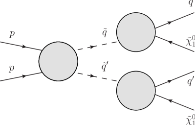
We present an analysis of the signature via squark–squark
production and direct decay into the lightest neutralino, ,
in next-to-leading order QCD within the framework of the minimal supersymmetric standard model.
In our approximation the produced squarks are treated
on shell. Thus, the calculation of production and decay factorizes.
In this way, we provide a consistent, fully differential calculation of
NLO QCD factorizable corrections to the given processes.
Clustering final states into partonic jets, we investigate the experimental
inclusive signature for several benchmark scenarios.
We compare resulting differential distributions with leading-order
approximations rescaled by a flat K-factor and examine a possible impact for cut-and-count
searches for supersymmetry at the LHC.
MPP-2012-106
1 Introduction
Supersymmetry (SUSY) [1] is one of the most appealing scenarios for physics beyond the Standard Model (SM), which the ongoing experiments at the Large Hadron Collider (LHC) are searching for. SUSY, predicting new states with masses at the TeV-scale or below, provides an elegant solution to the hierarchy problem, and gauge coupling unification can be achieved naturally. In addition, many realizations of SUSY, particularly the Minimal Supersymmetric Standard Model (MSSM), provide a viable dark matter candidate assuming the lightest SUSY particle (LSP) to be stable due to R-parity conservation. Furthermore, the MSSM is in accordance with the measured values of the muon anomalous magnetic moment and with electroweak precision observables, and also with a light Higgs boson as indicated by the ATLAS and CMS experiments [2, 3].
Within the MSSM and assuming conserved R-parity, SUSY particles (sparticles) are produced in pairs,
and related searches have been performed at LEP, the Tevatron, and the LHC using various
final-state signatures. Due to their color charge, squark and gluino production typically
gives the largest contribution to an inclusive SUSY cross section at a hadron collider
like the LHC. Assuming the lightest neutralino to be the LSP,
produced squarks and gluinos eventually decay into the neutralino which leaves the
detectors unobserved. This results in the general experimental signature of jets+missing
energy, which is one of the signatures that
has been searched for by the experiments at the LHC. Within the
constrained MSSM (CMSSM) resulting limits can be used to exclude squarks and
gluinos with masses below [4, 5]. Exact exclusion
limits, however, depend on the detailed structure of the underlying model parameters
and become much weaker, e.g., in parameter regions with compressed spectra where
final-state jets do not pass the cuts applied in the experimental searches
[6, 7, 8].
Precise and reliable theoretical predictions for squark and gluino production are
necessary for several reasons: – to set accurate exclusion limits, –
to possibly refine experimental search strategies in problematic parameter regions, and
– in case of discovery, to determine the parameters of the underlying model
[9].
The last point becomes more important as generic mass
bounds for squarks and gluinos are pushed to higher values and many of the
proposed sophisticated methods (see e.g.[10] for a review) for parameter
determination might not be feasible with low signal statistics due to a rather heavy
spectrum.
Until now precision studies of sparticle production at the LHC have focussed on inclusive
cross sections, without taking into account phase-space cuts that have to be applied in any
experimental analysis. Although these inclusive quantities are of fundamental interest,
both for exclusion limits and for parameter determination, they are not directly
observable in high-energy collider experiments. Furthermore, precise knowledge of
distributions of the decay products might help to determine the fundamental parameters
of the model [10, 11] or even permits the measurements of the
spin of the new particles [12, 13] and thereby helps
to discriminate SUSY models from possible other extensions of the SM with
similar signatures [14, 15]. Thus, a fully differential
prediction including higher-orders in all relevant stages of the process (eventually
matched to a NLO parton shower) is desirable.
In this paper we systematically study squark–squark production and the subsequent
decay into the lightest neutralino at next-to-leading order (NLO) in QCD. Final state
partons are clustered into jets and thus, we provide, for the first time at NLO, a fully differential
description of the physical signature via on-shell squark-squark
production and decay. In principle, our calculation does not depend on the hierarchy
between the squarks and the gluino. However, in our numerical evaluation we only
consider benchmark points where the mass of all light flavour squarks is smaller
than the gluino mass ; otherwise the decay of a squark into a gluino and
a quark would be dominant. Investigating the squark-squark channel should be
understood as a first step towards a fully differential prediction for all sparticle
production channels at NLO. It is, however, also of practical importance, since
from recent searches at the LHC mass bounds
for squarks and gluinos are generically pushed to higher values and here squark–squark
production (initiated from valence-quarks) yields the dominant channel [16].
First leading order (LO) cross section predictions for squark and gluino production processes were already made many years ago [17, 18, 19, 20, 21] and are reviewed in [22]. Also the calculation of NLO corrections in perturbative QCD has been performed quite some time ago [23, 24, 25, 26]. These corrections can be large (, depending on the process and the parameters) and have to be included in any viable phenomenological study due to the otherwise enormous scale uncertainties (including NLO corrections the scale uncertainty on inclusive cross sections is typically reduced to an order of ). Besides the scale uncertainty, PDF uncertainties dominate the error of theoretical predictions of sparticle production processes. In a very recent publication [27] general guidelines for the systematic treatment of these errors are presented.
Already in [25] differential distributions at NLO are presented for the produced squarks and gluinos. Here, NLO correction factors (K-factors) look rather flat in phase space. Therefore, in the experimental analyses, they are used as a global multiplicative factor to the LO cross section. However, a systematic study of the differential behaviour of these K-factors has never been performed. Furthermore, in [25] and in the corresponding public computer code Prospino 2 [28], which can calculate LO cross sections and NLO K-factors efficiently, NLO corrections for squark–squark production are always summed over the various flavour and chirality combinations of the produced (light-flavour) squarks. Realistic physical observables do depend on the chiralities through the decay modes which are in general quite different. In this work we treat the individual squark chirality and flavour configurations independently. One goal of our paper is to investigate the quality of these approximations: using flat K-factors and averaging on squark masses.
More recently also results beyond NLO in QCD were calculated,
based on resummation techniques
[29, 30, 31, 32, 33, 34, 35, 36]. These corrections increase the inclusive
cross section by about and further reduce the scale uncertainty.
Moreover, electroweak contributions can also give sizeable corrections.
At leading order
they were first calculated in [37, 38] and at NLO in
[39, 40, 41, 42, 43, 44, 45]. In detail, those corrections depend strongly
on the model parameters and on the flavour/chiralities of the squarks.
A similar amount of work has been put into the calculation of higher order corrections to decays of (coloured) sparticles, with focus mainly on the integrated decay widths and branching ratios. NLO QCD corrections to the decay of light squarks into neutralinos and charginos were first calculated in [46, 47] and to heavy squarks also in [47] and in [48]. Corrections to the total decay width of light squarks are in general moderate (below ) and can change sign, depending on the involved mass ratios. However, for very small mass splittings between the decaying squark and the neutralinos/charginos these corrections increase significantly. Higher-order corrections to the decay of top-squarks are in general sizeable, but they depend strongly on the mixing in the heavy squark sector. Related to this mixing also decays into weak gauge bosons or Higgs bosons can become relevant [49, 50], receiving large higher order corrections [51, 52, 53]. Decays of a gluino into a light squark and a quark at NLO QCD together with the decay of a light squark into a gluino and a quark have been calculated in [54]. Corresponding decays involving stops were presented in [55]. All these decays including their NLO QCD corrections have been implemented in the public computer programs SDECAY [56] and SUSY-HIT [57].
Besides NLO QCD, also NLO electroweak corrections to squark decays into neutralinos and charginos
have been investigated in the literature [58, 59] and can give
sizeable contributions. These corrections often compensate those from QCD on the level
of integrated decay widths, however, they depend strongly on the model parameters.
Corresponding NLO electroweak corrections for third generation squark decays have been studied in
[60, 61, 62, 63].
As already mentioned before, most of the discussed studies of higher-order corrections
focussed on inclusive observables or considered differential distributions in unphysical
final states, like unstable sparticles. Few studies were performed
investigating invariant mass distributions of SM particles emitted from cascade chains
including various higher-order corrections [64, 65]. Finally, in
[66, 67] production of sparticles was studied at tree
level matched to a parton shower including additional hard jets. In these works large
deviations from the LO prediction with or without showering were found particularly in
the high- tail for scenarios with compressed spectra. In this paper we go beyond these
estimates and provide a fully differential description of production and decay of
squark–squark pairs at NLO.
In the big picture of the complete calculation of NLO QCD corrections to , also , and
intermediate states can contribute to this signature. Already without systematically
including decays of the squarks, the calculation of NLO corrections to on-shell
production of such pairs of coloured sparticles carries problems of double counting.
Parts of NLO corrections to one final state can be identified as LO of another final
state where the decay is already included. The standard solution, used to avoid this
double counting problem, can not be straightforwardly extended to the
calculation where off-shell effects are included.
Moreover, complete NLO corrections to do not only include
factorizable contributions, i.e., contributions that can be classified as corrections to the
production or to the decays, but also non-factorizable contributions, where such
a separation is not possible. In this paper we analyze the factorizable NLO corrections to
squark–squark production and decay, which are expected to yield the dominant part of the
NLO contributions.
Non-factorizable effects and off-shell contributions
will be analyzed in a forthcoming publication, providing a consistent conceptual approach
and evaluating their numerical effects.
The outline of this paper is as follows. In section 2 the method of combining consistently production and decay at NLO in the narrow-width-approximation is described. In the subsequent two sections the calculation of all required ingredients of this combination is explained, with respect to the squark production processes in section 3, and to the squark decays in 4. In section 5 we present our numerical results for representative benchmark points, and conclude with a summary in section 6.
2 Method
We investigate the production of squark-squark pairs induced by proton-proton collisions, with subsequent decays of the squarks into the lightest neutralinos. Since we are interested in the experimental signature , all contributions from light-flavour squarks have to be included. Hence, the cross section is given by the sum over all independent flavour and chirality configurations,
| (1) |
Indices denote the flavours of the (s)quarks and their chiralities. At LO, the only partonic subprocesses that contribute to a given intermediate configuration or arise from quark and anti-quark pairs, respectively, and .
For simplifying the notation, we will write whenever the specification of flavour and chiralities is not required 111In this notation implies , but not vice versa.. Moreover, we will perform the discussion without the charge-conjugate subprocesses; they are, however, included in the final results.
In the considered class of processes, squarks appear as intermediate particles with mass and total decay width . In the limit , the narrow width approximation (NWA), their resonating contributions in the squared amplitude can be approximated by the replacement
| (2) |
for each squark with momentum .
At LO in NWA for scalar particles, the phase-space integration of the squared amplitude for the total cross section of the processes factorizes into a production and a decay part. At the partonic level, the LO cross section gets the following form,
| (3) |
with the LO partonic production cross section and the LO branching ratios for the squark decays into the lightest neutralino. A direct generalization of eq. (3) yields the cross section in a completely differential form, which can be written at the hadronic level as follows,
| (4) |
Therein, and denote the LO total widths of the two squarks; and are the respective differential decay distributions boosted to the moving frames of and .
The other basic ingredient, , is the hadronic differential production cross section, expressed in terms of the partonic cross section as a convolution
| (5) |
with the parton luminosity
| (6) |
where is the parton distribution function (PDF) at the scale of the quark with momentum fraction inside the proton. denotes the ratio between the squared center-of-mass energies of the partonic and hadronic processes, , and the kinematical production threshold corresponds to .
The NWA cannot be extended to the complete set of NLO QCD corrections to . Interactions between initial and final state quarks, for example, do not allow to split the process into on-shell production of squarks and subsequent decays. The subset of factorizable corrections, however, can be obtained in NWA, occurring as corrections to the production or to the decay processes, as illustrated in figure 1. In the present article we focus on this class of corrections, which are expected to be the dominant ones. In an upcoming article we will investigate the non-factorizable corrections and their numerical influence.
The differential cross section for on-shell production of squark–squark pairs and subsequent decays including the NLO factorizable corrections can be written as a formal expansion in ,
| (7) |
with the NLO contributions to cross section and widths
in obvious notation.
The LO term in the first line of eq. (2)
gets a global correction factor from the
NLO contribution to the total widths; the second and third line involve
the NLO corrections to the decay distributions and the production cross
section, respectively 222An analogous treatment has been used, e.g., for the calculation
of NLO corrections of top pair production and
decay [68, 69]..
In order to evaluate the terms contained in eq. (2), we produce, for all different combinations of light flavours and chiralities, weighted events for squark-squark production and squark decays. Production events for are generated in the laboratory frame. Decay events for and are generated in the respective squark rest frame. Finally, events are obtained by boosting the decay events from the squark rest frames, defined by the production events, into the laboratory frame. The weights of the events are obtained combining the different LO and NLO weights of production and decay according to eq. (2). Phenomenological results derived by these combinations are presented in section 5. The treatment of the various entries in eq. (2) is described in the following sections 3 and 4.
3 Squark–squark production
3.1 LO squark–squark production
Amplitudes and cross sections for squark production depend on the flavours
(indices ) and on the chiralities (indices ) of the squarks. We
consider light-flavour squarks only, treating quarks as massless.

If the two produced squarks are of the same flavour, the contributing Feynman diagrams correspond to - and -channel gluino exchange (figure 2). For squarks of the same chirality, the partonic cross section reads as follows,
| (8) |
where and are the usual Mandelstam variables for processes. For different chiralities, implies vanishing interference between the - and -channel diagrams, yielding
| (9) |
If the two squarks are of different flavours, there is no -channel exchange diagram; the partonic cross section for equal chiralities is hence given by
| (10) |
and for different chiralities by
| (11) |
Besides the dominating QCD contributions, there are also tree-level electroweak production channels [37, 44] with chargino and neutralino exchange, which can interfere with the QCD amplitude providing a contribution to the cross-section of . In principle these terms can be numerically of similar importance as the NLO QCD corrections we are investigating. For the present study, the electroweak contributions are neglected.
3.2 NLO squark–squark production
The NLO QCD corrections to squark–squark production have been known for many years [25] and an efficient public code (Prospino 2) is available for the calculation of total cross sections at NLO. However, in order to study systematically the signature emerging from production of squark–squark pairs and subsequent decays into the lightest neutralino, also the complete differential cross section is necessary. To this purpose, we perform an independent (re)calculation of the NLO QCD corrections, where we treat the masses for , and all chirality and flavour configurations independently. In [25] different squark chiralities are treated as mass degenerate and NLO contribution are always summed over all chirality and flavour combinations.
NLO calculations involve, in intermediate steps, infrared and collinear divergences. Since our calculation does not involve any diagrams with non-Abelian vertices, infrared singularities can be regularized by a gluon mass (). Collinear singularities, in analogy, can be regularized by a quark mass (), that is kept at zero everywhere else in the calculation. The cancellation of these two kinds of singularities is obtained by summing the virtual loop contributions and the real gluon bremsstrahlung part, with subsequent mass factorization in combination with the choice of the parton densities.
The complete NLO corrections to the differential cross section can be written symbolically in the following way,
| (12) |
With we denote the summed contributions from the renormalized virtual corrections and soft gluon emission; corresponds to initial state collinear gluon radiation including the proper subtraction term for the collinear divergences; denotes the remaining hard gluon emission outside the soft and collinear phase space regions. is the contribution from real quark emission from additional quark–gluon initial states contributing at NLO.
Technically, the calculation of the loop corrections and real radiation contributions is performed separately for every flavour and chirality combination, , with the help of FeynArts [70] and FormCalc [71, 72]. Appendix A shows a collection of the contributing Feynman diagrams. Loop integrals are numerically evaluated with LoopTools [71].
3.2.1 Virtual corrections and real gluon radiation
In the term the virtual and soft contributions are added at the parton level, according to
| (13) |
The fictitious gluon mass for infrared regularization cancels in the sum
of and .
At NLO, UV finiteness requires renormalization by inclusion of appropriate counterterms, which can be found explicitly in [40]. All mass and field renormalization constants are determined according to the on-shell scheme. The renormalization of the QCD coupling constant () has to be done in accordance with the scheme for in the PDFs, the scheme with five flavours; this corresponds to the renormalization constant [25]
| (14) |
with the UV divergence and the renormalization scale . is the leading term of the function for the QCD coupling in the MSSM. We choose to use dimensional regularization for the calculation. This breaks the supersymmetric Slavnov-Taylor identity that relates the vertex function and the vertex function at one-loop order. However, this identity can be restored (see [25, 73]) by an extra finite shift of the coupling in the vertex with respect to in the vertex,
| (15) |
The second term in eq. (3.2.1) contains the contributions from real gluon emission integrated over the soft-gluon phase space with . It is similar to the case of soft-photon emission [74, 75], yielding a multiplicative correction factor to the LO cross section. In the case of gluons, however, the color structures are different for emission from and channel diagrams and hence the various bremsstrahlung integrals enter the cross section with different weights. Accordingly, we decompose the partonic LO cross section for in the following way in obvious notation,
| (16) |
where the coefficients for the individual channels can be easily read off from the LO cross sections in eqs. (8)–(11). Defining for incoming and for outgoing particles, the soft gluon contribution at partonic level can be written as follows, using the label assignment ,
| (17) |
The involve the bremsstrahlung integrals
and the weight factors . Explicit
expressions are listed in eq. (43) of Appendix B.
still depends on the quark mass () owing to the initial-state collinear singularities. This dependence cancels by adding the real collinear radiation term resulting from gluon emission into the hard collinear region and mass factorization for the PDFs via adding a proper subtraction term,
| (18) |
The collinear gluon emission into a narrow cone around the emitting particle yields the following contribution that corresponds to the results of [76] with the replacement ,
| (19) |
The luminosity and the partonic cross section can be found in eqs. (45) and (46) of Appendix B.
The subtraction term for phase-space slicing, in accordance with the scheme, can be written in the following way,
| (20) |
Finally, we have to add from the residual hard gluon emission outside the collinear region, which cancels the dependence on the slicing parameters for the soft and for the collinear region.
3.2.2 Real quark radiation
The corrections to get also a contribution
from the gluon-initiated subprocesses and
, which
also have to be included for a consistent treatment of NLO PDFs.
Diagrams for these two subprocesses can be divided into resonant
(figure 3(a) and 4(a)) and non-resonant
(figure 3(b) and 4(b)) diagrams, where in
the resonant diagrams the intermediate gluino can be on-shell.
This resonant production channel via on-shell gluinos corresponds
basically to LO production of a squark–gluino pair (with
subsequent gluino decay). Such contributions are generally classified as squark–gluino
production and have to be removed here
333The same type of problem is discussed, e.g., in [77]
in the context of NLO corrections
to single top quark production, where quark radiation creates
configurations corresponding to top quark pair production..
In a general context, combining production and decay for all colored SUSY particles ( and ), also off-shell configurations from resonant diagrams appear. In this context, the off-shell contributions from resonant diagrams in figure 3(a) and 4(a) can, in the same way, be classified as production and decay of squark–gluino pairs.
The most important difference in calculations with and without including decays is the role of the colored supersymmetric particles. In one case they belong to the final state, in the other one they are intermediate states. Thus, due to the quark radiation at NLO, a separation of squark–gluino and squark–squark channel contributions to is only an intermediate organisational instrument. It is important to remember that our NLO calculation of the production of squark–squark pairs is meant as a necessary ingredient of eq. (2). Our primary goal is the consistency of the calculation at NLO of the full process with decays included and not only of the production of squarks.
In the following, we address the structure of the various terms
contributing to the real quark radiation and describe
two different approaches to perform the
subtraction of the contributions corresponding to squark–gluino production
(with subsequent gluino decay).
In the case of different flavours , there are two parton processes which provide NLO differential cross sections for real quark emission, given by
| (21) | ||||
where overline represents the usual summing and averaging of external helicities and colours and is the usual phase-space element for three particles in the final state. and correspond to the diagrams of figure 3(a) and figure 3(b), respectively, and and to those of figure 4(a) and figure 4(b).
For the case of equal flavours , we have
| (22) |
with from the diagrams of figure 3(a) and
figure 4(a), which we will call in this case and ;
is the part from the diagrams of figure 3(b)
and figure 4(b).
The term
appears only for equal chiralities () and flavors of the squarks.
We describe the subtractions for the case with equal flavor;
analogous arguments apply to the different-flavor case.


(a) (b)


(a) (b)
We refer to two strategies, used already in the literature 444The DR and DS schemes defined here are almost equal to the approaches extensively studied in [77]., to avoid the double-counting of terms contained also in the calculation of the squark–gluino channel contribution to :
-
•
DS: Diagram Subtraction,
-
•
DR: Diagram Removal.
In the DS scheme the contribution from the LO on-shell production of a squark–gluino pair with the gluino decaying into a squark is removed:
| (23) |
In eq. (3.2.2),
is the phase-space with three particles in the final state
applying consistently the on-shell condition
for the two different resonant cases.
Eq. (3.2.2) is conceptually equal to the DS scheme
explained in [77] and the “Prospino scheme” in [25, 78];
in practice there is a small difference with respect to our approach, which
is explained in more detail in appendix D. We subtract at global level exactly what we would obtain from LO
on-shell production of a squark–gluino pairs with the gluino decaying
into a squark. This is done by producing two different sets of events
corresponding to the two lines of eq. (3.2.2), respectively.
In [25, 77, 78] a local
subtraction of the on-shell contribution involving a mapping or
reshuffling of momenta from the general
phase-space into an equivalent on-shell configuration is
performed. These two implementations of the DS scheme give slightly
different results even in the limit .
The threshold conditions and
in the local subtraction, together with the convolution of the PDFs and the precise
on-shell mapping, produce small differences from numerical results of the global subtraction. The DS scheme, both in the local approach discussed in [77] and in the global approach, defined in eq. (3.2.2), is gauge invariant in the limit . The decay width of the gluino is used as a numerical regulator and not as a physical parameter.
In an extreme approach, the quark radiation calculation could even be
completely excluded from the NLO corrections in the squark–squark channel.
Then, all diagrams, resonant and non-resonant,
constituting a gauge invariant subset,
have to be included in the squark–gluino production and decay channel
(in this way, we would alter the organisational separation of squark/gluino channels).
Since the term
contains initial state collinear singularities, also the subtraction
term of the PDFs has to be excluded and computed within the squark–gluino channel.
It is worth to mention, that even if we want to include in all production and decay channels only on-shell configurations for the resonant intermediate supersymmetric particles (as performed here for the squark–squark channel), quark radiation in the NLO corrections introduces unavoidably off-shell contributions.
The DR scheme represents, in a certain sense, an intermediate step between the DS scheme and a complete removal as explained above. Here, one removes, from a diagrammatic perspective, the minimal set of contributions in the squared amplitude that contain a resonant gluino. In our calculation this results in
| (24) |
In the different flavor cases the third term in eq. (24) does not appear. Comparing eq. (24) with eq. (22), it is clear that the removed terms are and .
In the definition of DR given in [77] also the interference term is removed
(with a study of the impact of the inclusion of this contribution),
whereas we keep this interference term.
Although the DR scheme formally violates gauge invariance, a consistent description is
achieved when the procedure presented here is combined
with off-shell contributions.
It should not be forgotten that the narrow-width approximation, both in the DR and the DS scheme
is not an exact description in any case; as an approximation it has a natural uncertainty arising
from missing off-shell contributions and non-factorizable NLO corrections.
These will be studied in a forthcoming paper.
In our numerical results we basically employ the DR scheme, however, we
compare it with results in the DS scheme,
both for inclusive K-factors and for differential distributions.
Finally, for the practical calculation of the real quark radiation contributions, in both schemes one has to perform the phase space integration over the final state quark. The squared non-resonant terms lead, as mentioned before, to initial state collinear singularities. Again, these singular terms have to be subtracted since they are factorized and absorbed into the PDFs. Like in the case of gluon radiation, we divide the emission of a quark into a collinear and a non-collinear region (since no IR singularities occur, a separation into soft and hard quark emission is not required),
| (25) |
The non-collinear contribution
| (26) |
contains as given in eq. (51). The collinear emission together with the subtraction terms for the PDFs instead can be written as follows,
4 Squark decay
4.1 Squark decay at LO
The LO decay width for a squark decaying into a neutralino and a quark, , depends on the flavour and chirality of the squark. For the width can be written as follows,
| (28) |
The coupling constants can be expressed in terms of the isospin and the charge of the quark, together with the neutralino mixing matrix including the electroweak mixing angle through and ,
| (29) | ||||
| (30) | ||||
| (31) |
For a scalar particle decaying in its rest frame there is no preferred direction, and hence the differential decay distribution is isotropic. For squark decays into neutralino and quark, the decay distribution is thus simply given by
| (32) |
with polar angle and azimuth referring to the quark momentum.
4.2 NLO squark decay distribution
The differential decay width for at NLO is obtained in analogy to the steps in section 3.2 by adding the virtual loop corrections and the real gluon bremsstrahlung contribution from the soft, collinear, and hard non-collinear phase space regions, yielding the full NLO contribution in the form
| (33) |
The virtual corrections for correspond to the two vertex loop diagrams in figure 5(a) and the vertex counter term (indicated by the cross in figure 5(a)), which consists of the wave-function renormalization constants of the external quark and squark line. As for the production amplitudes, the renormalization constants are determined in the on-shell renormalization scheme. Details on the vertex counter term can be found in [40], and the explicit analytical expression is given in eq. (54) of Appendix C.


(a) (b)
The term can be calculated by the same strategy as for , yielding
| (34) |
where the are defined in eq. (44).
Collinear divergences now emerge from the final state. Making again use of the results of [76], the collinear emission of gluons with energy larger than into a cone with opening angle yields the contribution
| (35) | ||||
where , , and , the maximum energy available for the quark in the squark rest frame. Gluons with are recombined with the emitter quark into a quark with momentum . In general, differential distributions in the quark momenta are dependent on the slicing parameter . However, this dependence will disappear once a jets algorithm that is much more inclusive in the recombination of quarks and gluons, is applied (see section 5).
The contribution from real emission of hard gluons () at large angles () is evaluated by numerical integration of the squared matrix elements, obtained from the diagrams in figure 5(b).
4.3 Total decay width
The total squark decay width at LO is obtained by summing the partial decay widths of the 6 different possible decay channels into neutralinos and charginos (assuming always ). The partial decay widths into neutralinos are given directly by eq. (28). For charginos, the partial decay widths are also described by the formula (28), with the specification and
| (36) |
for the coupling constants. Here, are the mixing matrices in the chargino sector.
For the total decay width at NLO, one has to calculate the NLO QCD corrections for each channel, which can be done analytically performing the full phase space integration over the three-particle final state with the radiated gluon and adding the loop contributions. The six partial decay widths contributing to at NLO can be expressed in terms of their respective LO result and a NLO form factor , eq. (57), which depends only on the mass ratios of the involved massive particles,
| (37) |
The result for in[47] is confirmed by our independent derivation. Details can be found in Appendix C. In the threshold limit the correction in eq. (57) becomes very large and the fixed-order calculation is not reliable (relative corrections remain finite only after proper resummation, see for example [65]). However, for all parameter points considered in the numerical evaluation in section 5 the corrections are still sufficiently small and threshold problems are negligible.
5 Phenomenological evaluation
Let us now turn to the numerical evaluation of the process under consideration. In the following, we first specify in 5.1 the input parameters and benchmark scenarios we consider in our numerical evaluation. Then, in 5.2 a brief introduction to all considered distributions and observables is given. Finally, in 5.3, we present our numerical results in three different ways. Firstly, we compare our results for inclusive production of squark–squark pairs with Prospino 2 and investigate inclusive K-factors for different chirality and flavour combinations. Secondly, we present several differential distributions for various benchmark scenarios and center-of-mass energies. Thirdly, we investigate the impact of the considered higher-order corrections on total event rates and thus on cut-and-count searches for supersymmetry at the LHC.
5.1 Input parameters
Standard Model input parameters are chosen according to [22],
| (38) |
We use the PDF sets CTEQ6.6 [79]
interfaced via the LHAPDF package [80]
both for LO and NLO contributions. The strong coupling constant
is also taken from this set of PDFs. Factorization scale
and renormalization scale are, if not stated otherwise, set to a common
value, , with being the average mass
of all light-flavour squarks of a given benchmark point.
For SUSY parameters, we refer to three different benchmark scenarios. First, we
investigate the well studied CMSSM parameter point SPS1a [81].
Although being practically excluded by recent searches at the
LHC [4, 5, 82],
this point still serves as a valuable benchmark to
compare with numerous numerical results available in the literature.
Second, we study the benchmark point CMSSM10.1.5 introduced in [83].
Due to its larger parameter, compared to SPS1a, squark and gluino masses
are considerably larger, resulting in a generally reduced production cross section at the
LHC. Not excluded yet, this parameter point can be tested in the near future. The
overall spectrum, though shifted to larger masses, is very similar to the one of SPS1a.
Third, we consider a phenomenological benchmark point defined at the scale .
We follow the definitions of [83], where such a point sits on a line called
p19MSSM1. It can be parametrized by essentially one parameter, the
gaugino mass parameter . A unified parameter for the gluino and the
light-generations sfermion soft masses is fixed
to on this line and we choose
for our benchmark scenario p19MSSM1A. All other masses and
parameters as well as the soft masses for the first two generation right-handed
sleptons are at a higher scale and irrelevant for our analysis.
This benchmark point is chosen to study a particular parameter region with rather light
squarks and gluinos which is difficult to exclude experimentally. Due to a small mass splitting between the and the light squarks (and gluino) resulting jets tend to be very soft and thus escape the experimental analyses. Particularly in such parameter regions precise theoretical prediction of the resulting SUSY signal including
higher orders on the level of distributions seems to be necessary for a conclusive study.
| benchmarkpoint | |||||
|---|---|---|---|---|---|
| SPS1a | 100 GeV | 250 GeV | 100 GeV | 10 | |
| 10.1.5 | 175 GeV | 700 GeV | 0 | 10 |
| benchmarkpoint | ||||||
|---|---|---|---|---|---|---|
| p19MSSM1A | 300 GeV | 2500 GeV | 360 GeV | 0 | 10 |
| benchmarkpoint | ||||||
|---|---|---|---|---|---|---|
| SPS1a | 563.6 | 546.7 | 569.0 | 546.6 | 608.5 | 97.0 |
| 10.1.5 | 1437.7 | 1382.3 | 1439.7 | 1376.9 | 1568.6 | 291.3 |
| p19MSSM1A | 339.6 | 394.8 | 348.3 | 392.7 | 414.7 | 299.1 |
| benchmarkpoint | ||||||
|---|---|---|---|---|---|---|
| SPS1a | ||||||
| 10.1.5 | ||||||
| p19MSSM1A | ||||||
Parameters of the CMSSM benchmark scenarios are defined universally at the GUT scale and are shown in table 1. They act as boundary conditions for the renormalization group running of the soft-breaking parameters down to the SUSY scale . This running is performed with the program SOFTSUSY [84] which also calculates physical on-shell parameters for all SUSY mass eigenstates. We use the resulting on-shell parameters directly as input for our calculation. Low scale soft input parameters for the p19MSSM1A benchmark scenario are given in table 2. The physical spectrum is equivalently calculated with SOFTSUSY. For all considered benchmark scenarios we summarize relevant low energy physical masses in table 3. Due to non-vanishing Yukawa corrections implemented in SOFTSUSY the physical on-shell masses for second-generation squarks are slightly different from their first-generation counterparts. To simplify our numerical evaluation we set all second-generation squark masses to their first-generation counterparts. We checked that in the results this adjustment is numerically negligible. However, the general setup of our calculation is independent of this choice. For all considered benchmark scenarios the gluino is heavier than all light flavour squarks . Thus, these squarks decay only into electroweak gauginos and quarks. For SPS1a and 10.1.5, right-handed squarks dominantly decay directly into the lightest neutralino (due to its bino nature). In contrary, left-handed squarks decay dominantly into heavier (wino-like) neutralinos and charginos, which subsequently decay via cascades into a , and only a small fraction decays directly into a . In this paper we only investigate the direct decay of any light flavour squark into the lightest neutralino. For point p19MSSM1A all neutralinos and charginos, but the lightest one, are heavier than any light-flavour squark. Thus, only the direct decay is allowed and all channels contribute equally to the signature under consideration.
In table 4 we list all needed total decay widths of the squarks at LO and NLO, calculated as explained in section 4. NLO corrections in the total decay widths are of the order of a few percent for all three benchmark scenarios 555 Numerically we observed a disagreement with the partial decay widths at NLO for p19MSSM1A obtained from SDECAY, despite the fact that the NLO contributions in SDECAY are based on the analytical results calculated in [47] and in Appendix C. After corresponding with the authors, this problem was solved by correcting a typo in SDECAY. We thank M. Mühlleitner for helpful discussions. . The total decay width of the gluino is calculated with SDECAY at LO and also listed in table 4. In the calculation presented here this width is not used explicitly. Instead, we numerically employ the limit . However we checked that, using the physical widths, all the results showed in the following present negligible differences.
Besides physical quantities, in our calculation phase-space slicing and regulator parameters
enter as inputs in the calculation of virtual and real NLO contributions, as explained in
sections 3 and 4.
In the results shown in this article we set ,
and , both for production and decay.
Numerically we checked carefully that varying their values our results remain unchanged on the level of individual
distributions once jets are recombined using a clustering algorithm, as explained below. We made sure that this holds
for all terms of eq. (2) individually.
5.2 Observables and kinematical cuts
The physical signature we have in mind when calculating on-shell squark production and decay into the lightest neutralino is . Numerical results of our calculation are presented in this spirit. In order to arrive at an experimentally well defined two-jet-signature we always employ the anti-[85] jet-clustering algorithm implemented in FastJet 3.0.2 [86]. Thus, we provide a realistic prediction on the level of partonic jets 666With the term partonic jets we mean that the jet-clustering-algorithm has been applied to events as produced from our calculation. No QCD showering or hadronization is included in the simulation.. In general we use a jet radius of , as in the SUSY searches performed by the ATLAS collaboration [5]. CMS instead uses a radius of [4]. We employ in the distributions and signatures used by CMS (i.e. particularly the distribution as described below). Although we did not perform a systematic study, our results seem to be independent of this choice. After performing the jet clustering we sort the partonic jets by their transverse momentum , and in the following analysis we keep only jets with
| (39) | ||||
| (40) |
Cuts of eq. (39) are used everywhere but in the observables used specifically by CMS (, as defined below), where cuts of eq. (40) are applied.
Before showing results for the experimental signature , we compare in section 5.3.1 values for NLO total cross sections of squark-squark production, without decay included, with results obtained from Prospino 2. In section 5.3.2 we investigate the effect of NLO corrections, for different benchmark points, on the following differential distributions:
-
•
the transverse momentum of the two hardest jets ,
-
•
the pseudorapidity of the two hardest jets ,
-
•
the missing transverse energy ,
-
•
the effective mass ,
-
•
the scalar sum of the of all jets (visible after cuts of eq. (40)), ,
-
•
the invariant mass of the two hardest jets ,
-
•
the cosine of the angle between the two hardest jets , which depends on the spin of the produced particles and therefore might help to distinguish SUSY from other BSM models [14],
-
•
, , introduced in [13] as a possible observable for early spin determination at the LHC,
- •
Searches for sparticle production performed by ATLAS are based on , and cuts; CMS instead uses to reduce SM backgrounds. In section 5.3.3 we examine NLO corrections in the resulting event rates after cuts. Explicitly we employ the following cuts used by ATLAS,
| (41) | ||||
in their two-jet analysis [5]. Here, denotes the angular separation between the two hardest jets and the direction of missing energy. Instead the CMS signal region [88] is defined as
| (42) | |||
where is calculated from .
5.3 Results
5.3.1 Inclusive cross sections
In table 5 we list inclusive LO cross sections and corresponding NLO
K-factors for the three benchmark scenarios SPS1a, 10.1.5, p19MSSM1A, varying the LHC center of mass
energy . K-factors, here and in the following, are always defined as ratios
between NLO and LO predictions, where both, as stated above, are calculated using the same
NLO PDFs and associated . On the one hand, we list inclusive cross sections,
, and K-factors for just the production of squark-squark
pairs summed over all flavour and chirality combinations. These K-factors are calculated
in the DR scheme defined in section 3.2.2. If not stated otherwise this scheme is
used in the following. On the other hand, we list cross section predictions
for combined production and decay at LO and the
corresponding NLO K-factors calculated using eq. (2),
again summed over all flavour and chirality combinations. Here, cuts defined in
eq. (39) are applied and cross sections are strongly decreased due to the
branching into the lightest neutralino. All K-factors of the combined process are
bigger than the corresponding K-factors of inclusive production. For point 10.1.5
(and thus rather heavy squarks) these increments are less than . For the
other two benchmark points (and thus smaller squark masses) increments in the
K-factors can be of the order of and increase with higher center of mass
energies. In general, however, K-factors decrease with higher center of mass energies
and increase with higher masses, both, for inclusive production and combined
production and decay.
| benchmark | [TeV] | ||||
|---|---|---|---|---|---|
| pb | pb | ||||
| SPS1a | pb | pb | |||
| pb | pb | ||||
| fb | fb | ||||
| 10.1.5 | fb | fb | |||
| fb | fb | ||||
| pb | pb | ||||
| p19MSSM1A | pb | pb | |||
| pb | pb |
In table 6 we compare the inclusive production with combined production
and decay for benchmark point 10.1.5 and a center of mass energy of .
Here, we list results for individual flavour and chirality combinations. In general, our
calculation is set up to treat all possible flavour and chirality
combinations independently. However, for simplicity and to save computing time we always
sum combinations with identical masses and matrix elements into 16 channels, both, for
production and in the combination. This categorization follows the four
possibilities discussed in section 3.1. For example, the channel also
includes (and as everywhere else in this paper, the charge
conjugated processes). Similarly, the channel also includes , and ; and the channel also includes .
K-factors, both, in just the production and in the combined result, vary by up to
between different channels. Thus, an independent treatment seems adequate, as in general,
squarks of different chiralities and thus different channels have very different decays and
kinematic distributions. This can easily be seen from the very different order of magnitude of
the various values of in table 6. As already
seen in table 5, K-factors increase comparing inclusive production and the
combined result (where the cuts given in eq. (39) are applied).
| channel | ||||||
|---|---|---|---|---|---|---|
| [fb] | [fb] | [fb] | [fb] | |||
| sum |
In table 7 we compare the different schemes defined in 3.2.2.
In order to also consistently compare with Prospino 2 results, we set, just here,
the mass of all squarks to the average mass for all bechmark points.
In table 7 we show LO cross-sections and NLO K-factors from our calculation in the DR scheme,
, and in the DS scheme, . We also
list K-factors obtained from Prospino 2, , where we
adjusted Prospino 2 to use the same set of PDFs and definition of the strong coupling
as in our calculation. The use of an average mass results in a small shift
in the LO cross section and also in the NLO K-factor between table 5
and table 7.
Numerical differences between K-factors in the DR scheme and the DS scheme
are of the order of a few percent for SPS1a and p19MSSM1A and negligible for 10.1.5, as, for
a heavier spectrum the gluon contribution in the PDFs is suppressed. Differences between
and originate in the different
on-shell subtraction approach. We checked numerically, excluding real quark radiation
altogether, that inclusive NLO corrections from our calculation and results from
Prospino 2 are in perfect agreement.
| benchmark | [TeV] | ||||
|---|---|---|---|---|---|
| pb | |||||
| SPS1a | pb | ||||
| pb | |||||
| fb | |||||
| 10.1.5 | fb | ||||
| fb | |||||
| pb | |||||
| p19MSSM1A | pb | ||||
| pb |
5.3.2 Differential Distributions
Now we turn to the investigation of differential distributions in various observables.
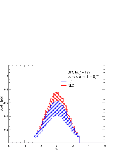
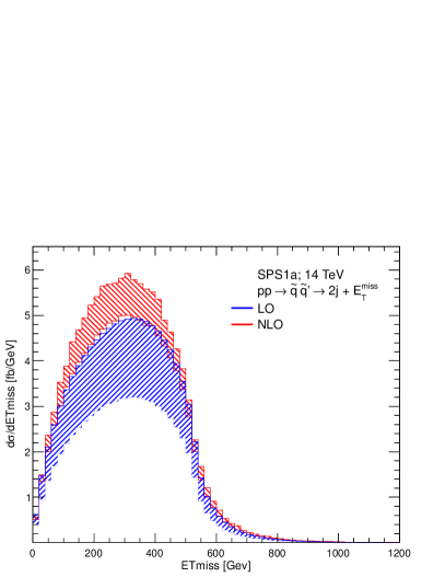
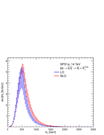
First, we compare the differential scale dependence between our LO and NLO
prediction. We do this by varying at the same time renormalization and factorization scale
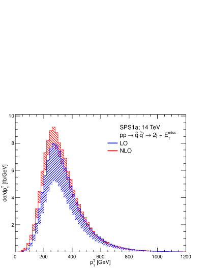
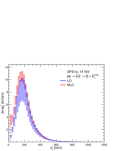
between , with . For SPS1a and an
energy of resulting LO and NLO bands are shown in blue and red in
figure 6 for differential distributions in and . Clearly, in all considered distributions the scale
dependence and thus the theoretical uncertainty is greatly reduced by our NLO calculation.
At the same time, one should also note that large parts of the NLO bands are outside the
LO bands. Still, for example in the distributions, in the high-pT tail the NLO bands
move entirely inside the LO bands.
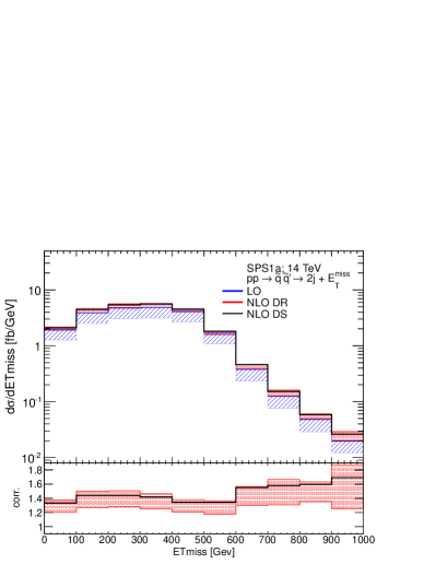
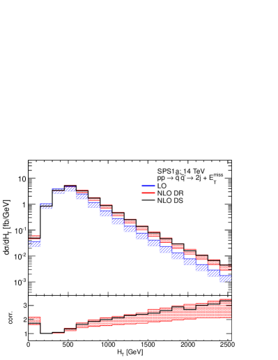
Second, in figure 7 we illustrate the difference between the schemes introduced
in section 3.2.2 for the benchmark point SPS1a and a center of mass
energy . In figure 7 we show distributions in and . These are the distributions where we observe the largest deviations between the DS and DR schemes.
The upper part of these plots show the same band plots as already displayed at the bottom
of 6, however in a log scale. In the lower part we show, for the DR scheme,
the ratio of the NLO results at and over
the LO results at . We also display the ratio between the NLO result
in the DS scheme and the LO result, both at the central . In these two
distributions the difference between the two schemes increases in the tail of the distributions.
However the DS scheme remains within the theoretical uncertainty of the DR scheme. As explained
the chosen distributions and show the largest differences we observe for the
benchmark points and energies considered.
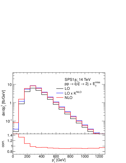
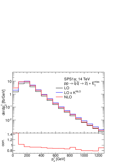
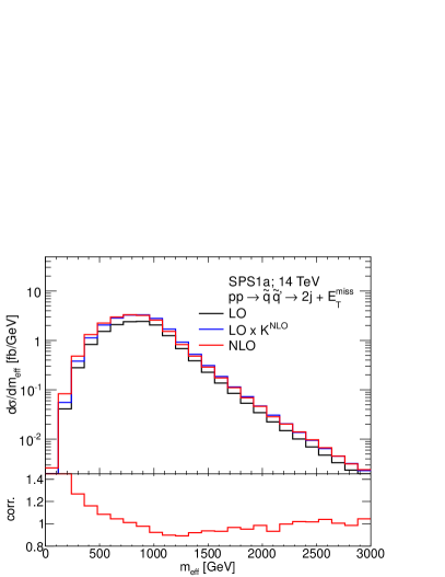
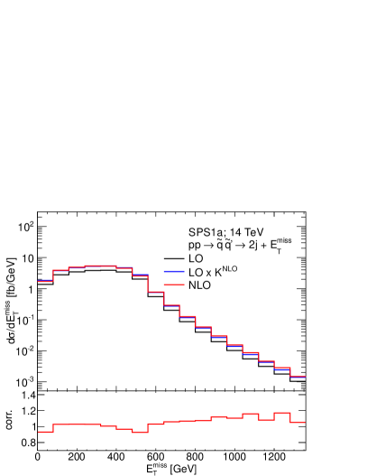
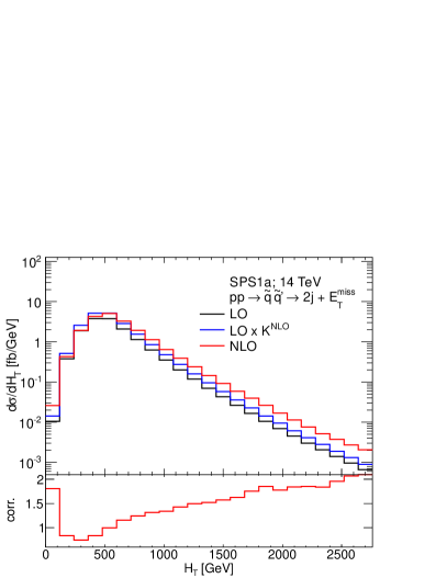
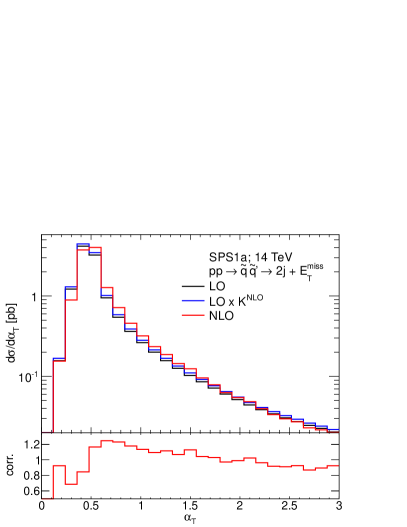
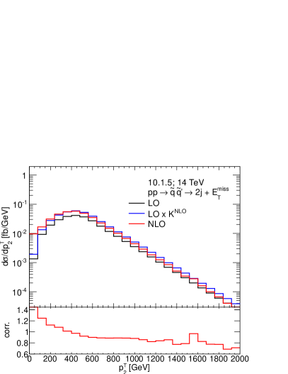
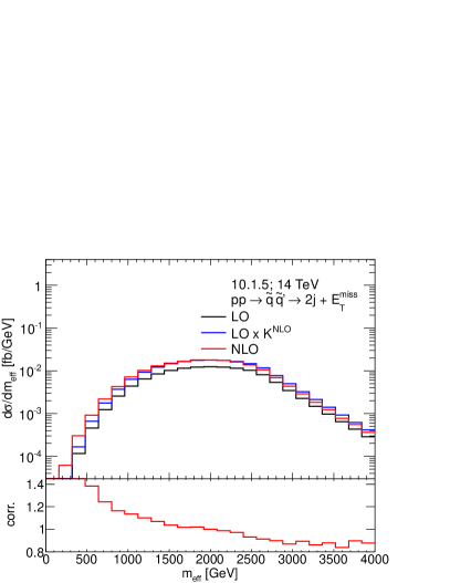
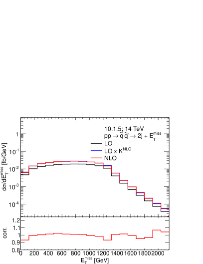
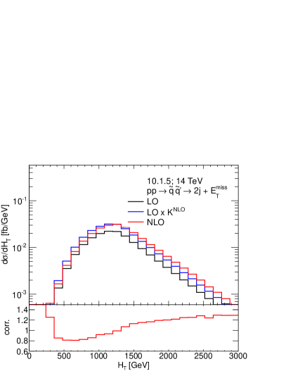
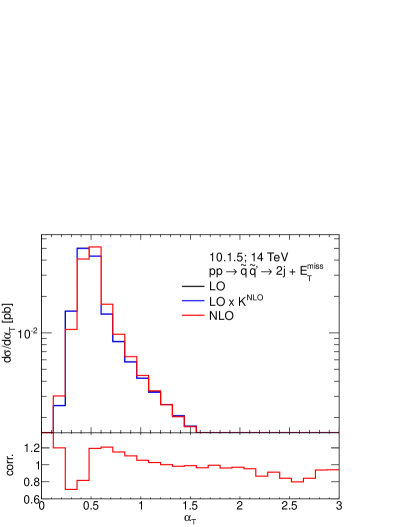
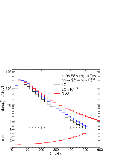
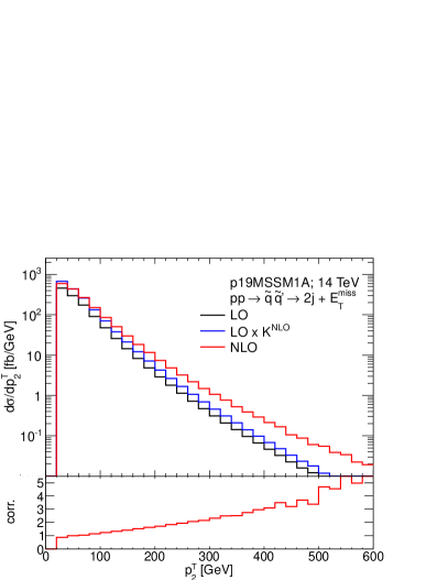
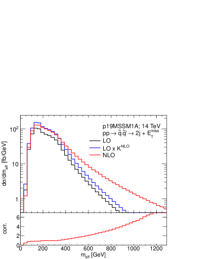
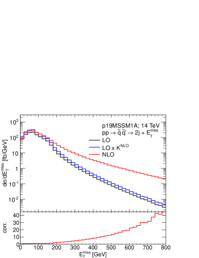
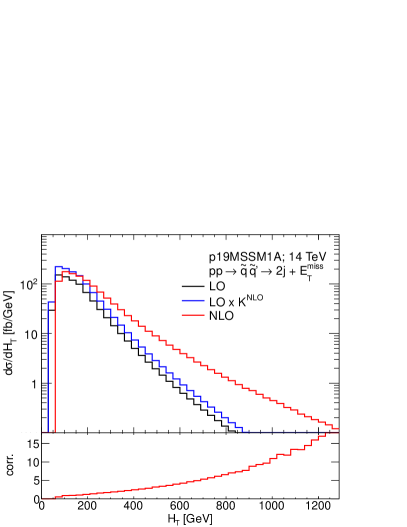
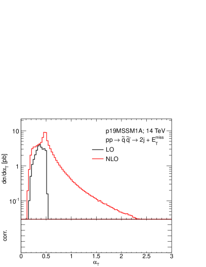
Third, we investigate the change in the shape of distributions relevant for searches for
supersymmetry at the LHC when going from LO to NLO. Here, we present distributions for
a center of mass energy . Lower center of mass energies show qualitatively
the same behaviour. For benchmark point SPS1a plots are shown in figure 8,
for 10.1.5 in figure 9 and for p19MSSM1A in figure 10. We present
distributions in , , , (all in fb/GeV), where the ATLAS
jet choice and cuts of eq. (39) are applied. Also distributions in
(in fb/GeV) and in (in pb) are displayed, where the CMS jet choice
and corresponding cuts of eq. (39) are applied. In the distribution,
events are reclustered into two pseudojets and a cut of is applied. In the
upper
part of any plot we show each distribution at LO in black, NLO in red and in blue the
LO prediction rescaled by the ratio, , between the integrated NLO and
LO result. In the lower part of any plot we show the NLO divided by the rescaled
distribution. In this way we present corrections
purely in the shape and not in the normalization of the distributions.
For SPS1a and 10.1.5 corrections are qualitatively very similar and rather flat for
, and , as expected from [25]. Corrections in the (inclusive) distribution grow for larger and can be sizeable. This can be explained from
the high- behaviour of the contribution from hard real gluon radiation to this observable.
Corrections to the shape of the observable change sign at the physical boundary [87]
and fall off continuously in the signal region .
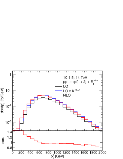
Looking at the distributions of p19MSSM1A in figure 10 a completely different
behaviour of the NLO corrections cannot be missed. The tail of the , ,
and distributions completely departs from the LO predictions. This
can be understood from the following considerations. Due to the small mass splitting between
squarks and the for benchmark point p19MSSM1A, jets from squark decays tend to be soft.
Now, the of an additional jet (which can not be distinguished from the decay jets) from
hard gluon radiation in the production can easily be of the same order as the ones from squark
decays and result in the given distortions. Such a behaviour for compressed spectra was already partly
discussed in [67], where sparticle production and decay including additional hard jets matched to a parton shower
was investigated. We verified our findings by comparing LO predictions plus real hard gluon radiation
in the production stage with a corresponding calculation performed with MadGraph 5 [90].
The tail of the considered distributions can adequately only be described by additional gluon radiation,
which should thus be seen as the LO prediction for these phase-space regions. Still, only our
full NLO calculation allows a consistent treatment of the entire distributions. Turning to the
distribution, clearly shapes of LO and NLO prediction are different and, here, we refrain from
showing explicitly corrections in the shape or a rescaled LO prediction.
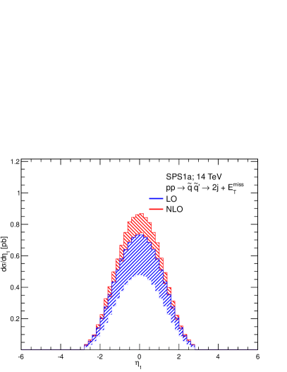
Next to the distributions shown in figures 8, 9 and
10, we also investigated pseudorapidity distributions of the two hardest jets .
Here, in the relevant region corrections in the shapes are
always smaller than about for all benchmark scenarios and energies.
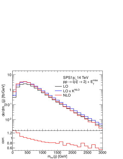
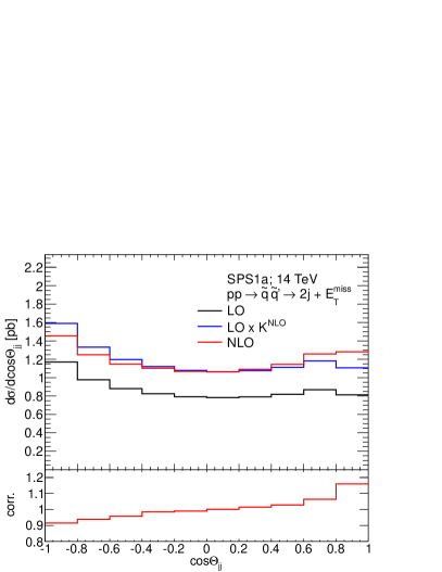
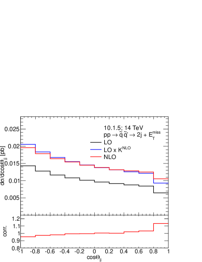
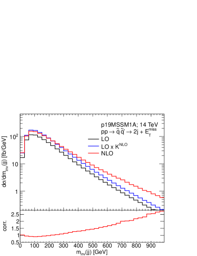
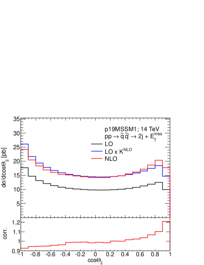
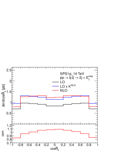
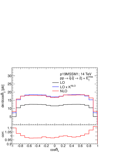
In figure 11 we turn our attention towards angular distributions between the
two hardest jets. On the left we show distributions in the invariant mass of the two
hardest jets , on the right distributions in the cosine of the angle between the two
hardest jets are presented. Again results are shown for all three benchmark points and a
center of mass energy . Corrections in these distributions can be quite large.
In general, in the full NLO results one observes an increase for small angles between
the two hardest jets (up to in the distributions). In the
high-invariant-mass tail for SPS1a and 10.1.5 corrections are negative and grow
to in the considered invariant mass range. Such corrections could potentially
be absorbed into a dynamical renormalization/factorization scale definition, e.g., ;
in-detail investigation is left to future work. In the invariant mass distribution of p19MSSM1A we observe
the same deviation of the NLO result from the LO shape as already
discussed above.
Finally, in figure 12 we investigate NLO corrections to the distribution for the benchmark points SPS1a (top left), 10.1.5 (top right) and p19MSSM1A (bottom) at a center of mass energy of . Corrections up to are observable. Still, the general shape and thus the potential for extraction of spin information about the intermediate squarks seems to be robust under higher order corrections.


5.3.3 Event rates
After investigating inclusive cross sections and differential distributions, we now proceed to event rates, i.e., cross sections integrated on signal regions defined to reduce background contributions. By this study, we want to quantify a possible impact of our calculation on current searches for supersymmetry and future measurements of event rates at the LHC.
In table 8 we list cross sections after applying cuts of eq. (41) and in table 9 cross sections after applying cuts of eq. (42). We show LO and NLO cross sections for all three benchmark points and all three energies together with resulting K-factors. For comparison we again list inclusive K-factors of just production, already shown in table 5. From these results, a fully differential description of all squark and gluino channels including NLO effects in production and decay seems inevitable for a conclusive interpretation of SUSY searches (or signals) at the LHC. Numbers in table 8 and table 9 again show that, for compressed spectra like p19MSSM1A, a pure LO approximation is unreliable for a realistic phenomenological description of the experimental signatures considered here. Furthermore, as already suggested in [91] and expected from the differential distributions shown in section 5.3.2, in particular interpretations based on seem to be highly affected by higher order corrections.
| benchmarkpoint | Energy [TeV] | ||||
|---|---|---|---|---|---|
| pb | pb | ||||
| SPS1a | pb | pb | |||
| pb | pb | ||||
| fb | fb | ||||
| 10.1.5 | fb | fb | |||
| fb | fb | ||||
| fb | fb | ||||
| p19MSSM1A | fb | fb | |||
| pb | pb |
| benchmarkpoint | Energy [TeV] | ||||
|---|---|---|---|---|---|
| pb | pb | ||||
| SPS1a | pb | pb | |||
| pb | pb | ||||
| pb | pb | ||||
| 10.1.5 | fb | fb | |||
| fb | fb | ||||
| pb | pb | ||||
| p19MSSM1A | pb | pb | |||
| pb | pb |
6 Conclusions
In this paper we presented a study of squark–squark production and the subsequent squark decay into the lightest neutralino at the LHC, providing for the first time fully differential predictions for the experimental signature at NLO in QCD. For the calculation, each flavour and chirality configuration of the squarks has been treated individually, allowing the combination of production cross sections and decay distributions in a consistent way.
We studied inclusive cross sections, differential distributions for jet observables, and experimental signatures with cuts, illustrating the effect of the NLO contributions. In general, the NLO corrections are important. In particular, NLO effects going beyond a rescaling with a global -factor can in general not be neglected for setting precise limits on the sparticle masses and model parameters; they become specially important in model classes with compressed spectra. At the same time, the theoretical uncertainty on the level of differential distributions is reduced by our calculation.
Although the present study is dedicated to the simplest squark decay mode, the fully differential description facilitates also the study of more complex final states including electroweak decay chains at the same level of the QCD perturbative order. Since the calculational framework is fully exclusive also with respect to flavour and chiralities, it can easily be merged with the electroweak contributions of LO and NLO.
Acknowledgments.
This work was supported in part by the Research Executive Agency of the European Union under the Grant Agreement PITN-GA-2010-264564 (LHCPhenonet). We are grateful to M. Flowerdew, P. Graf, T. Hahn, E. Mirabella, F.D. Steffen and particularly A. Landwehr for valuable discussions.Appendix A Diagrams of NLO corrections
Here, for completeness, we display all relevant diagrams used in our NLO calculation of squark-squark production.
The contribution of some of them vanish under the assumption . For
example, this is the case for the diagram on the line when
; any helicity state of the quark in the propagator can interact either with
or with but not with both of them.


Appendix B Formulae for soft and collinear radiation
B.1 Soft radiation
The soft-bremsstrahlung correction factor in eq. (17) involves the kinematical factors from (16) and phase space integrals [75, 44]. Keeping a finite quark mass only in the mass-singular terms, yields the following expressions for the production process , where the labels correspond to the assignment , , , and ,
| (43) | ||||
with , ,
For the decay process , the corresponding expressions for in the decay width eq. (34) read as follows, with the the label assignment , (and ),
| (44) | ||||
B.2 Collinear radiation
This appendix collects the entries in eqs. (19) and (3.2.1) for hard collinear radiation. They are taken from [76] and [92] with the replacement .
The (unintegrated) parton luminosity entering both the collinear gluon emission (19) and the subtraction term (3.2.1) is given by
| (45) |
The partonic cross section for the collinear emission of a gluon into the cones with opening angle around the two quarks in the initial state can be written as follows,
| (46) |
with . The variable is the ratio between the momenta of the emitter parton after and before the emission.
At the parton level, the -dependent part of the subtraction term for one quark is given by
| (47) |
involving the factorization scale , whereas the -independent part
| (48) |
contains also the soft-gluon phase space cut .
In an analogous way, the (unintegrated) parton luminosity for collinear quark radiation in eq. (3.2.2) is given by
| (49) |
involving also the gluon distribution function .
Collecting in one formula the collinear cone emission of a quark and the subtraction term (last term in the brackets of eq. (B.2)), one finds
| (50) |
with the gluon–quark splitting function .
Finally, the parton luminosity for non-collinear quark radiation is
| (51) |
Appendix C NLO corrections to the squark decay width
In section 4.3 we need the NLO corrections to the decay width , where is either a neutralino or a chargino, and a light quark. Here we perform the derivation of the correction factor, following the steps of the former calculation [47], but keeping explicitly the dependence on the masses for the collinear singularities and for the IR singularities. The NLO corrections in eq. (37) can be expressed in terms of a form factor , which receives four contributions,
| (52) |
namely loop corrections involving gluons and gluinos , the counterterm contribution , and the contribution from real gluon emission .
Keeping and as independent mass parameters for the singular terms, in dimensional reduction and can be written as follows,
| (53) | ||||
| (54) |
where , and denotes the UV divergence, cf. eq. (14).
is free of soft, collinear, and UV singularities, hence it is not affected by the choice of regulators; it is identical to the result in [47] and we do not repeat it here.
The part from real gluon emission, integrated over the full phase space, can be expressed with the help of the bremsstrahlung integrals given in [75], evaluated in the limit except for the mass-singular terms. The fully integrated decay width for can be written as follows,
| (55) | |||
with from eq. (28) and (36). The phase space integrals are given by
| (56) |
With these expressions, eq. (55) yields for the real gluon part of in eq. (52),
| (57) | |||||
Combining all four contributions in eq. (52) we obtain a compact analytical expression for the form factor , which agrees with the result in [47],
| (58) | |||||
where for the function is given by
and for one has
Appendix D Comparison between local and global diagram subtraction schemes
Here, expanding the discussion in section 3.2.2, we want to elucidate the differences between the implementations of the DS scheme in the global approach, as used in this paper, and in the local approach, as used e.g. in [25, 77, 78]. In the following discussion we consider the contribution from the resonant diagrams of figure 4(a). In a notation similar to the one of appendix B.1 of [25], the contribution to the partonic cross section emerging from these diagrams can be written as
| (59) |
where is the differential cross section in (the squared invariant mass of and ) without the squared gluino propagator. Given the squared total energy in the partonic center of mass , the maximum allowed value for is .
In the global approach the contribution from on-shell production is subtracted by substituting with
| (60) |
i.e. subtracting exactly the total cross section for on-shell production of multiplied by the branching ratio of .
In the local approach, before phase-space integration, evaluated in the on-shell gluino configuration
| (61) |
is subtracted in the numerator of the integrand of eq. (59),
| (62) |
In this parton level example the integral can be analytically calculated. For and , i.e. in the region where subtraction is required, it yields
Comparing in this way the global and local approach for the DS subtraction we find
| (64) |
Hence, even in the limit , the two approaches differ by a finite term depending on the physical phase space boundaries, see also [93]. This can be understood from the fact that the approximation of the Breit-Wigner distribution in the integrand of is strictly valid only for an integration over the entire real axis. Moreover, the result in eq. (64) can be altered if the mapping in the local subtraction is performed before the integration of the other phase space variables. This mapping is not uniquely defined and can lead to further differences. At the hadronic level the numerical differences between the two approaches can be of the order of a few per mill of the on-shell production. Thus, depending on the parameter region, few per-cent differences can appear for the NLO relative corrections. For example, for SPS1a and , corrections for the cross section arising from eq. (64) amount to of and to of , since . For different flavour and chirality configurations these corrections vary, they are, however, of the same order. Finally, we want to note that both the local and the global approach can be extended to a fully differential level.
References
- [1] J. Wess and B. Zumino, Supergauge Transformations in Four-Dimensions, Nucl. Phys. B70 (1974) 39–50.
- [2] ATLAS Collaboration, G. Aad et al., Observation of a new particle in the search for the Standard Model Higgs boson with the ATLAS detector at the LHC, Phys. Lett. B 716, 1 (2012) [arXiv:1207.7214].
- [3] CMS Collaboration, S. Chatrchyan et al., Observation of a new boson at a mass of 125 GeV with the CMS experiment at the LHC, Phys. Lett. B 716, 30 (2012) [arXiv:1207.7235].
- [4] CMS Collaboration, S. Chatrchyan et. al., Search for Supersymmetry at the LHC in Events with Jets and Missing Transverse Energy, Phys.Rev.Lett. 107 (2011) 221804, [arXiv:1109.2352].
- [5] ATLAS Collaboration, G. Aad et. al., Search for squarks and gluinos using final states with jets and missing transverse momentum with the ATLAS detector in sqrt(s) = 7 TeV proton-proton collisions, Phys.Lett. B710 (2012) 67–85, [arXiv:1109.6572].
- [6] T. J. LeCompte and S. P. Martin, Compressed supersymmetry after 1/fb at the Large Hadron Collider, Phys. Rev. D85 (2012) 035023, [arXiv:1111.6897].
- [7] M. Asano, T. Bringmann, and C. Weniger, Indirect dark matter searches as a probe of degenerate particle spectra, Phys. Lett. B709 (2012) 128–132, [arXiv:1112.5158].
- [8] A. Strubig, S. Caron, and M. Rammensee, Constraints on the pMSSM from searches for squarks and gluinos by ATLAS, JHEP 05 (2012) 150, [arXiv:1202.6244].
- [9] H. K. Dreiner, M. Kramer, J. M. Lindert, and B. O’Leary, SUSY parameter determination at the LHC using cross sections and kinematic edges, JHEP 04 (2010) 109, [arXiv:1003.2648].
- [10] A. J. Barr and C. G. Lester, A Review of the Mass Measurement Techniques proposed for the Large Hadron Collider, J. Phys. G37 (2010) 123001, [arXiv:1004.2732].
- [11] D. Miller, P. Osland, and A. Raklev, Invariant mass distributions in cascade decays, JHEP 0603 (2006) 034, [hep-ph/0510356].
- [12] J. M. Smillie and B. R. Webber, Distinguishing Spins in Supersymmetric and Universal Extra Dimension Models at the Large Hadron Collider, JHEP 10 (2005) 069, [hep-ph/0507170].
- [13] G. Moortgat-Pick, K. Rolbiecki, and J. Tattersall, Early spin determination at the LHC?, Phys. Lett. B699 (2011) 158–163, [arXiv:1102.0293].
- [14] G. Hallenbeck, M. Perelstein, C. Spethmann, J. Thom, and J. Vaughan, Model Discrimination with the CMS Detector: a Case Study, Phys. Rev. D79 (2009) 075024, [arXiv:0812.3135].
- [15] J. Hubisz, J. Lykken, M. Pierini, and M. Spiropulu, Missing energy look-alikes with 100 pb-1 at the LHC, Phys. Rev. D78 (2008) 075008, [arXiv:0805.2398].
- [16] S. Mrenna, A Closer Look at the 2011 cMSSM Results from CMS, arXiv:1110.4078.
- [17] G. L. Kane and J. P. Leveille, Experimental Constraints on Gluino Masses and Supersymmetric Theories, Phys. Lett. B112 (1982) 227.
- [18] P. R. Harrison and C. H. Llewellyn Smith, Hadroproduction of Supersymmetric Particles, Nucl. Phys. B213 (1983) 223. [ERRATUM-ibid.B223:542,1983].
- [19] E. Reya and D. P. Roy, Supersymmetric particle production at p anti-p collider energies, Phys. Rev. D32 (1985) 645.
- [20] S. Dawson, E. Eichten, and C. Quigg, Search for Supersymmetric Particles in Hadron - Hadron Collisions, Phys. Rev. D31 (1985) 1581.
- [21] H. Baer and X. Tata, Component formulae for hadroproduction of left-handed and right-handed squarks, Phys. Lett. B160 (1985) 159.
- [22] Particle Data Group, K. Nakamura et. al., Review of particle physics, J. Phys. G37 (2010) 075021.
- [23] W. Beenakker, R. Hopker, M. Spira, and P. M. Zerwas, Squark production at the Tevatron, Phys. Rev. Lett. 74 (1995) 2905–2908, [hep-ph/9412272].
- [24] W. Beenakker, R. Hopker, M. Spira, and P. M. Zerwas, Gluino pair production at the Tevatron, Z. Phys. C69 (1995) 163–166, [hep-ph/9505416].
- [25] W. Beenakker, R. Hopker, M. Spira, and P. M. Zerwas, Squark and gluino production at hadron colliders, Nucl. Phys. B492 (1997) 51–103, [hep-ph/9610490].
- [26] W. Beenakker, M. Kramer, T. Plehn, M. Spira, and P. M. Zerwas, Stop production at hadron colliders, Nucl. Phys. B515 (1998) 3–14, [hep-ph/9710451].
- [27] M. Kramer et. al., Supersymmetry production cross sections in pp collisions at sqrts = 7 TeV, arXiv:1206.2892.
- [28] W. Beenakker, R. Hopker, and M. Spira, PROSPINO: A program for the PROduction of Supersymmetric Particles In Next-to-leading Order QCD, hep-ph/9611232.
- [29] U. Langenfeld and S.-O. Moch, Higher-order soft corrections to squark hadro- production, Phys. Lett. B675 (2009) 210–221, [arXiv:0901.0802].
- [30] A. Kulesza and L. Motyka, Threshold resummation for squark-antisquark and gluino- pair production at the LHC, Phys. Rev. Lett. 102 (2009) 111802, [arXiv:0807.2405].
- [31] A. Kulesza and L. Motyka, Soft gluon resummation for the production of gluino-gluino and squark-antisquark pairs at the LHC, Phys. Rev. D80 (2009) 095004, [arXiv:0905.4749].
- [32] W. Beenakker et. al., Soft-gluon resummation for squark and gluino hadroproduction, JHEP 12 (2009) 041, [arXiv:0909.4418].
- [33] W. Beenakker et. al., Supersymmetric top and bottom squark production at hadron colliders, JHEP 08 (2010) 098, [arXiv:1006.4771].
- [34] M. Beneke, P. Falgari, and C. Schwinn, Threshold resummation for pair production of coloured heavy (s)particles at hadron colliders, Nucl. Phys. B842 (2011) 414–474, [arXiv:1007.5414].
- [35] W. Beenakker et. al., NNLL resummation for squark-antisquark pair production at the LHC, JHEP 01 (2012) 076, [arXiv:1110.2446].
- [36] P. Falgari, C. Schwinn, and C. Wever, NLL soft and Coulomb resummation for squark and gluino production at the LHC, JHEP 06 (2012) 052, [arXiv:1202.2260].
- [37] S. Bornhauser, M. Drees, H. K. Dreiner, and J. S. Kim, Electroweak Contributions to Squark Pair Production at the LHC, Phys. Rev. D76 (2007) 095020, [arXiv:0709.2544].
- [38] A. Arhrib, R. Benbrik, K. Cheung, and T.-C. Yuan, Higgs boson enhancement effects on squark-pair production at the LHC, JHEP 02 (2010) 048, [arXiv:0911.1820].
- [39] W. Hollik, M. Kollar, and M. K. Trenkel, Hadronic production of top-squark pairs with electroweak NLO contributions, JHEP 02 (2008) 018, [arXiv:0712.0287].
- [40] W. Hollik and E. Mirabella, Squark anti-squark pair production at the LHC: the electroweak contribution, JHEP 12 (2008) 087, [arXiv:0806.1433].
- [41] W. Hollik, E. Mirabella, and M. K. Trenkel, Electroweak contributions to squark–gluino production at the LHC, JHEP 02 (2009) 002, [arXiv:0810.1044].
- [42] M. Beccaria, G. Macorini, L. Panizzi, F. M. Renard, and C. Verzegnassi, Stop-antistop and sbottom-antisbottom production at LHC: a one-loop search for model parameters dependence, Int. J. Mod. Phys. A23 (2008) 4779–4810, [arXiv:0804.1252].
- [43] E. Mirabella, NLO electroweak contributions to gluino pair production at hadron colliders, JHEP 12 (2009) 012, [arXiv:0908.3318].
- [44] J. Germer, W. Hollik, E. Mirabella, and M. K. Trenkel, Hadronic production of squark-squark pairs: The electroweak contributions, JHEP 08 (2010) 023, [arXiv:1004.2621].
- [45] J. Germer, W. Hollik, and E. Mirabella, Hadronic production of bottom-squark pairs with electroweak contributions, JHEP 05 (2011) 068, [arXiv:1103.1258].
- [46] K.-i. Hikasa and Y. Nakamura, Soft breaking correction to hard supersymmetric relations: QCD corrections to squark decay, Z. Phys. C70 (1996) 139–144, [hep-ph/9501382]. [ERRATUM-ibid.C71:356,1996].
- [47] A. Djouadi, W. Hollik, and C. Junger, QCD corrections to scalar quark decays, Phys. Rev. D55 (1997) 6975–6985, [hep-ph/9609419].
- [48] S. Kraml, H. Eberl, A. Bartl, W. Majerotto, and W. Porod, SUSY-QCD corrections to scalar quark decays into charginos and neutralinos, Phys. Lett. B386 (1996) 175–182, [hep-ph/9605412].
- [49] A. Bartl, W. Majerotto, and W. Porod, Squark and gluino decays for large tan beta, Z. Phys. C64 (1994) 499–508. [ERRATUM-ibid.C68:518,1995].
- [50] A. Bartl et. al., Bosonic decays of stop(2) and sbottom(2), Phys. Lett. B435 (1998) 118–124, [hep-ph/9804265].
- [51] A. Bartl et. al., SUSY-QCD corrections to stop and sbottom decays into W+- and Z0 bosons, Phys. Lett. B419 (1998) 243–252, [hep-ph/9710286].
- [52] A. Arhrib, A. Djouadi, W. Hollik, and C. Junger, SUSY Higgs boson decays into scalar quarks: QCD corrections, Phys. Rev. D57 (1998) 5860–5870, [hep-ph/9702426].
- [53] A. Bartl et. al., SUSY - QCD corrections to top and bottom squark decays into Higgs bosons, Phys. Rev. D59 (1999) 115007, [hep-ph/9806299].
- [54] W. Beenakker, R. Hopker, and P. M. Zerwas, SUSY QCD decays of squarks and gluinos, Phys. Lett. B378 (1996) 159–166, [hep-ph/9602378].
- [55] W. Beenakker, R. Hopker, T. Plehn, and P. M. Zerwas, Stop decays in SUSY-QCD, Z. Phys. C75 (1997) 349–356, [hep-ph/9610313].
- [56] M. Muhlleitner, A. Djouadi, and Y. Mambrini, SDECAY: A Fortran code for the decays of the supersymmetric particles in the MSSM, Comput. Phys. Commun. 168 (2005) 46–70, [hep-ph/0311167].
- [57] A. Djouadi, M. M. Muhlleitner, and M. Spira, Decays of Supersymmetric Particles: the program SUSY-HIT (SUspect-SdecaY-Hdecay-InTerface), Acta Phys. Polon. B38 (2007) 635–644, [hep-ph/0609292].
- [58] J. Guasch, J. Sola, and W. Hollik, Yukawa coupling corrections to scalar quark decays, Phys. Lett. B437 (1998) 88–99, [hep-ph/9802329].
- [59] J. Guasch, W. Hollik, and J. Sola, Fermionic decays of sfermions: A complete discussion at one-loop order, JHEP 10 (2002) 040, [hep-ph/0207364].
- [60] A. Arhrib and R. Benbrik, Third generation sfermions decays into Z and W gauge bosons: Full one-loop analysis, Phys. Rev. D71 (2005) 095001, [hep-ph/0412349].
- [61] A. Arhrib and R. Benbrik, Complete one-loop analysis to stop and sbottom decays into Z and W+- bosons, Afr. J. Math. Phys. 3 (2006) 85–91, [hep-ph/0511116].
- [62] Q. Li, L. G. Jin, and C. S. Li, Supersymmetric electroweak corrections to heavier top squark decay into lighter top squark and neutral Higgs boson, Phys. Rev. D66 (2002) 115008, [hep-ph/0207363].
- [63] C. Weber, K. Kovarik, H. Eberl, and W. Majerotto, Complete one-loop corrections to decays of charged and CP- even neutral Higgs bosons into sfermions, Nucl. Phys. B776 (2007) 138–169, [hep-ph/0701134].
- [64] M. Drees, W. Hollik, and Q. Xu, One-loop calculations of the decay of the next-to-lightest neutralino in the MSSM, JHEP 02 (2007) 032, [hep-ph/0610267].
- [65] R. Horsky, M. Kramer, A. Muck, and P. M. Zerwas, Squark Cascade Decays to Charginos/Neutralinos: Gluon Radiation, Phys. Rev. D78 (2008) 035004, [arXiv:0803.2603].
- [66] T. Plehn, D. Rainwater, and P. Z. Skands, Squark and gluino production with jets, Phys. Lett. B645 (2007) 217–221, [hep-ph/0510144].
- [67] J. Alwall, S. de Visscher, and F. Maltoni, QCD radiation in the production of heavy colored particles at the LHC, JHEP 02 (2009) 017, [arXiv:0810.5350].
- [68] K. Melnikov and M. Schulze, NLO QCD corrections to top quark pair production and decay at hadron colliders, JHEP 08 (2009) 049, [arXiv:0907.3090].
- [69] J. M. Campbell and R. K. Ellis, Top-quark processes at NLO in production and decay, arXiv:1204.1513.
- [70] T. Hahn, Generating Feynman diagrams and amplitudes with FeynArts 3, Comput. Phys. Commun. 140 (2001) 418–431, [hep-ph/0012260].
- [71] T. Hahn and M. Perez-Victoria, Automatized one-loop calculations in four and D dimensions, Comput. Phys. Commun. 118 (1999) 153–165, [hep-ph/9807565].
- [72] T. Hahn and C. Schappacher, The implementation of the minimal supersymmetric standard model in FeynArts and FormCalc, Comput. Phys. Commun. 143 (2002) 54–68, [hep-ph/0105349].
- [73] W. Hollik and D. Stockinger, Regularization and supersymmetry-restoring counterterms in supersymmetric QCD, Eur. Phys. J. C20 (2001) 105–119, [hep-ph/0103009].
- [74] G. ’t Hooft and M. Veltman, Scalar One Loop Integrals, Nucl.Phys. B153 (1979) 365–401.
- [75] A. Denner, Techniques for calculation of electroweak radiative corrections at the one loop level and results for W physics at LEP-200, Fortschr. Phys. 41 (1993) 307–420, [arXiv:0709.1075].
- [76] U. Baur, S. Keller, and D. Wackeroth, Electroweak radiative corrections to W boson production in hadronic collisions, Phys. Rev. D59 (1999) 013002, [hep-ph/9807417].
- [77] S. Frixione, E. Laenen, P. Motylinski, B. R. Webber and C. D. White, Single-top hadroproduction in association with a W boson, JHEP 0807, 029 (2008), [arXiv:0805.3067].
- [78] T. Binoth et. al., Automized Squark-Neutralino Production to Next-to-Leading Order, Phys. Rev. D84 (2011) 075005, [arXiv:1108.1250].
- [79] P. M. Nadolsky, H.-L. Lai, Q.-H. Cao, J. Huston, J. Pumplin, et. al., Implications of CTEQ global analysis for collider observables, Phys.Rev. D78 (2008) 013004, [arXiv:0802.0007].
- [80] M. R. Whalley, D. Bourilkov, and R. C. Group, The Les Houches Accord PDFs (LHAPDF) and Lhaglue, hep-ph/0508110.
- [81] B. C. Allanach et. al., The Snowmass points and slopes: Benchmarks for SUSY searches, Eur. Phys. J. C25 (2002) 113–123, [hep-ph/0202233].
- [82] M. J. Dolan, D. Grellscheid, J. Jaeckel, V. V. Khoze, and P. Richardson, New Constraints on Gauge Mediation and Beyond from LHC SUSY Searches at 7 TeV, JHEP 1106 (2011) 095, [arXiv:1104.0585].
- [83] S. AbdusSalam, B. Allanach, H. Dreiner, J. Ellis, U. Ellwanger, et. al., Benchmark Models, Planes, Lines and Points for Future SUSY Searches at the LHC, Eur.Phys.J. C71 (2011) 1835, [arXiv:1109.3859].
- [84] B. C. Allanach, SOFTSUSY: a program for calculating supersymmetric spectra, Comput. Phys. Commun. 143 (2002) 305–331, [hep-ph/0104145].
- [85] M. Cacciari and G. P. Salam, Dispelling the myth for the jet-finder, Phys.Lett. B641 (2006) 57–61, [hep-ph/0512210].
- [86] M. Cacciari, G. P. Salam, and G. Soyez, FastJet user manual, Eur. Phys. J. C72 (2012) 1896, [arXiv:1111.6097].
- [87] L. Randall and D. Tucker-Smith, Dijet Searches for Supersymmetry at the LHC, Phys. Rev. Lett. 101 (2008) 221803, [arXiv:0806.1049].
- [88] CMS Collaboration, V. Khachatryan et. al., Search for Supersymmetry in pp Collisions at 7 TeV in Events with Jets and Missing Transverse Energy, Phys.Lett. B698 (2011) 196–218, [arXiv:1101.1628].
- [89] B. C. Allanach, Impact of CMS Multi-jets and Missing Energy Search on CMSSM Fits, Phys. Rev. D83 (2011) 095019, [arXiv:1102.3149].
- [90] J. Alwall, M. Herquet, F. Maltoni, O. Mattelaer, and T. Stelzer, MadGraph 5 : Going Beyond, JHEP 1106 (2011) 128, [arXiv:1106.0522].
- [91] Z. Usubov, Looking for Squark Pair Production in the Early LHC Data, arXiv:1005.5062.
- [92] K.-P. Diener, S. Dittmaier, and W. Hollik, Electroweak higher-order effects and theoretical uncertainties in deep-inelastic neutrino scattering, Phys.Rev. D72 (2005) 093002, [hep-ph/0509084].
- [93] D. Berdine, N. Kauer and D. Rainwater, Breakdown of the Narrow Width Approximation for New Physics, Phys. Rev. Lett. 99, 111601 (2007) [hep-ph/0703058].