Implications of nonlinearity for spherically symmetric accretion

Abstract

We subject the steady solutions of a spherically symmetric accretion flow to a time-dependent radial perturbation. The equation of the perturbation includes nonlinearity up to any arbitrary order, and bears a form that is very similar to the metric equation of an analogue acoustic black hole. Casting the perturbation as a standing wave on subsonic solutions, and maintaining nonlinearity in it up to the second order, we get the time-dependence of the perturbation in the form of a Liénard system. A dynamical systems analysis of the Liénard system reveals a saddle point in real time, with the implication that instabilities will develop in the accreting system when the perturbation is extended into the nonlinear regime. The instability of initial subsonic states also adversely affects the temporal evolution of the flow towards a final and stable transonic state.

I Introduction

The classical model of steady spherically symmetric accretion Bondi (1952) is a mathematical problem of conservative and compressible hydrodynamics. This model has acquired a paradigmatic status in studies on astrophysical accretion, which, as a fluid flow, falls under the general class of nonlinear dynamics. The mathematical description of such fluid systems involves a momentum balance equation (with gravity as an external force in accretion), the continuity equation and a polytropic equation of state Frank et al. (2002). Set in full detail, the condition of momentum conservation in a fluid is a balance of dynamic effects, nonlinear effects and the effects of the pressure in a continuum system Landau and Lifshitz (1987). Some early studies on astrophysical accretion considered only the interplay between dynamics and nonlinearity (see Bondi (1952) and references therein), but in present studies, it is customary to ignore the dynamics and instead consider the effects of pressure, in what becomes a stationary flow. In either case, however, nonlinearity endures.

From the plethora of mathematical solutions of the stationary spherically symmetric compressible fluid flow, the ones of physical relevance are identified to be locally subsonic very far away from the accretor. Within the class of inflows obeying this outer boundary condition, there is an infinitude of globally subsonic solutions, along which a fluid element may reach the accretor with a low subsonic velocity. For the same outer boundary condition, a single critical solution stands out in a class by itself, and allows matter to reach the accretor with a high supersonic velocity, crossing the sonic horizon along the way. This is the unique transonic Bondi (1952) accretion solution. The exact fashion in which accreting matter reaches the accretor is related to the inner boundary condition of the inflow problem. If the accretor is a black hole, the infall process must be transonic Novikov and Thorne (1973); Shapiro and Teukolsky (1983). This is because a black hole has an event horizon instead of a physical surface, and thus precludes all possibility of a pressure build-up at small radii, which could otherwise have dominated over the free-fall conditions close to the accretor. The situation is not so clearly understood if the accretor has a hard surface like a neutron star or a white dwarf. For such an accretor, it is supposed that the accumulated matter will build up pressure near the surface and cause the supersonic flow to be shocked down to subsonic levels, although for a neutron star, all accreted matter might be “vacuum cleaned” away efficiently, making it easier for the flow to remain supersonic Petterson et al. (1980). Evidently then, the question of the inner boundary condition and an inflow trajectory in relation to it, is by no means a trivial one. Nevertheless, working with the stationary problem itself, Bondi (1952) invoked the physical criteria of the maximization of the accretion rate and the minimization of the total energy of the flow, to propose that the transonic solution would be the one selected by a fluid element to reach the accretor from a distant outer boundary. Bondi (1952), however, left a definitive conclusion regarding the realizability of the transonic solution to its stability.

The trouble with the transonic solution in the stationary regime is that its realizability is extremely vulnerable to even an infinitesimal deviation from the precisely needed boundary condition to generate the solution (Ray and Bhattacharjee, 2002). This difficulty may be overcome by considering the temporal evolution of global solutions towards the transonic state (Ray and Bhattacharjee, 2002; Roy and Ray, 2007), but there is no analytical formulation to solve the nonlinear partial differential equations governing the temporal evolution of the flow. So, much of all time-dependent studies in spherically symmetric accretion is perturbative and linearized in character, although some non-perturbative studies are also known (Ray and Bhattacharjee, 2002; Roy and Ray, 2007). The commonly accepted view to have emerged from the linearized approach is that perturbations on the flow do not produce any linear mode with an amplitude that gets amplified in time (Gaite, 2006), and that the perturbative method does not indicate the primacy of any particular class of solutions (Garlick, 1979). This is as far as could be said, working in the linear regime, but our general experience of any nonlinear system is that an understanding gained about it under linearized conditions can scarcely be imposed on circumstances dominated by nonlinearity. In this work we attempt to bridge the gap.

First we adopt a time-dependent radial perturbation scheme implemented originally by Petterson et al. (1980) and retain all orders of nonlinearity in the resulting equation of the perturbation. A most striking feature of this equation is that even on accommodating nonlinearity in full order, it conforms to the structure of the metric equation of a scalar field in Lorentzian geometry (Section III). This fluid analogue (an “acoustic black hole”), emulating many features of a general relativistic black hole, is a matter of continuing interest in fluid mechanics from diverse points of view (Moncrief, 1980; Unruh, 1981; Jacobson, 1991; Unruh, 1995; Visser, 1998; Bilić, 1999; Schützhold and Unruh, 2002; Das, 2004; Singha et al., 2005; Unruh and Schützhold, 2005; Volovik, 2005, 2006; Ray and Bhattacharjee, 2007a, b; Roy and Ray, 2007; Naskar et al., 2007; Das et al., 2007; Mach and Malec, 2008; Barceló et al., 2011; Robertson, 2012; Sarkar et al., 2014). Then we apply our nonlinear equation of the perturbation to study the stability of globally subsonic stationary solutions under large-amplitude time-dependent perturbations. Our motivation to do so lies in certain dynamic features of the flow. For the non-perturbative time evolution of the accreting system, the initial condition of the evolution is a globally subsonic state, with gravity subsequently driving the system to a transonic state, sweeping through an infinitude of intermediate subsonic states. So, to ensure an unhindered temporal convergence to a stable transonic trajectory, the stability of the subsonic states is crucial. In a numerical study, an instability in the subsonic states was observed by Stellingwerf and Buff (1978), who were consequently of the view that the subsonic flows would quickly change into the transonic flow. Our nonlinear perturbative analysis does agree with the fact that there is an instability in the subsonic states, but short of an exact non-perturbative analysis of all the nonlinear flow equations concerned (for which there exists no analytical prescription yet), it would be hasty to claim that the transonic state is indeed the final stable attractor state for the unstable subsonic states. The feasible analytical alternative, therefore, is to study the behaviour of the system under progressively higher orders (nonlinear orders) of time-dependence in the perturbative approach. We truncate all orders of nonlinearity beyond the second order in our equation of the perturbation. Following this, we integrate out the spatial dependence of the perturbation with the help of well-defined boundary conditions on globally subsonic flows (Petterson et al., 1980; Theuns and David, 1992). After this, we extract the time-dependent part of the perturbation and note with intrigue that it has the mathematical form of a Liénard system (Strogatz, 1994; Jordan and Smith, 1999) (Section IV). On applying the standard analytical tools of dynamical systems to study the equilibrium features of this Liénard system, we discover the existence of a saddle point in real time, whose implication is that the stationary background solutions will be unstable, if the perturbation is extended into the nonlinear regime (Section V). We also provide independent numerical support in favour of our analytical findings on the dynamics (Sections V & VI).

II The mathematical conditions of spherically symmetric accretion

The mathematical problem that was set up by Bondi (1952) himself and that is now taken up as a starting model in accretion-related texts (Chakrabarti, 1990; Frank et al., 2002), involves two coupled fields, the local flow velocity, $v$, and the local density, $\rho$, of the compressible accreting fluid. These two coupled fields are governed by the continuity equation,

$$\frac{\partial\rho}{\partial t}+\frac{1}{r^{2}}\frac{\partial}{\partial r}\left(\rho vr^{2}\right)=0,$$ (1)

and the inviscid Euler equation,

$$\frac{\partial v}{\partial t}+v\frac{\partial v}{\partial r}+\frac{1}{\rho}\frac{\partial P}{\partial r}+\Phi^{\prime}(r)=0,$$ (2)

tailored as they are, according to the requirements of spherical symmetry. In the latter equation, the local pressure, $P$, is expressed in terms of $\rho$, by invoking a general polytropic prescription, $P=k\rho^{\gamma}$, in which $\gamma$, the polytropic exponent, varies over the range (limited by isothermal and adiabatic conditions), $1\leq\gamma\leq c_{\mathrm{P}}/c_{\mathrm{V}}$, with $c_{\mathrm{P}}$ and $c_{\mathrm{V}}$ being the two coefficients of specific heat capacity of a gas (Chandrasekhar, 1939). The polytropic prescription is suited well for the study of open systems like astrophysical flows. Making use of both $P$ and $\rho$, we scale the bulk flow velocity, $v$, in terms of a natural hydrodynamic scale of speed, $c_{\mathrm{s}}$, which is the local speed of sound. This speed can be noted from $c_{\mathrm{s}}^{2}=\partial P/\partial\rho=\gamma k\rho^{\gamma-1}$. The non-self-gravitating bulk flow is driven by the external gravity of a central accretor, whose potential is $\Phi(r)$. In equation (2) the driving force arising due to this potential is implied by its spatial derivative (represented by the prime). In the case of stellar accretion, the flow is driven by the Newtonian potential, $\Phi(r)=-GM/r$. In studies of accretion onto a non-rotating black hole, it is often expedient to dispense with the rigour of general relativity, and instead use a pseudo-Newtonian potential Paczyński and Wiita (1980); Artemova et al. (1996) to mimic the general relativistic effects of Schwarzschild space-time geometry in a Newtonian construct of space and time (see Das and Sarkar (2001) and references therein). The choice of a pseudo-Newtonian potential, however, does not affect overmuch the general arguments regarding the stability of the flow.

With the functions, $P$ and $\Phi(r)$, specified thus, equations (1) and (2) give a complete description of the hydrodynamic flow in terms of the two fields, $v(r,t)$ and $\rho(r,t)$. The steady solutions of the flow are obtained from these dynamic variables by making explicit time-dependence disappear, i.e. $\partial v/\partial t=\partial\rho/\partial t=0$. The resulting differential equations, with full spatial derivatives only, can then be easily integrated to get the stationary global solutions of the flow (Bondi, 1952; Frank et al., 2002). A noticeable feature of these stationary solutions is that they are invariant under the transformation $v\longrightarrow-v$, i.e. the mathematical problems of inflows ($v<0$) and outflows ($v>0$) are identical in the steady state (Choudhuri, 1999). This invariance has adverse implications for critical flows in accretion processes. Critical solutions pass through saddle points in the stationary phase portrait of the flow (Ray and Bhattacharjee, 2002; Roy and Ray, 2007), but generating a stationary solution through a saddle point will be impossible by any physical means, because it calls for an infinite precision in the required outer boundary condition (Ray and Bhattacharjee, 2002). Nevertheless, criticality is not a matter of doubt in accretion processes (Bondi, 1952; Garlick, 1979; Shapiro and Teukolsky, 1983). The key to resolving this paradox lies in considering explicit time-dependence in the flow, because of which, as we note from equations (1) and (2), the invariance under the transformation, $v\longrightarrow-v$, breaks down. Obviously then, a choice of inflows $(v<0)$ or outflows $(v>0)$ has to be made at the very beginning (at $t=0$), and solutions generated thereafter will be free of all the difficulties associated with the presence of a saddle point in the stationary flow.

On imposing various boundary conditions on the steady integral solutions, multiple classes of flow result (Frank et al., 2002). Of these, the one that attracts attention in accretion studies obeys the boundary conditions, $v\longrightarrow 0$ as $r\longrightarrow{\infty}$ (the outer boundary condition) and $v>c_{\mathrm{s}}$ for small values of $r$. It is quite obvious that this solution is transonic in nature, with its bulk flow velocity overcoming the local speed of sound at a particular point in space, $r_{\mathrm{c}}$, the critical radius of the flow (Chakrabarti, 1990; Frank et al., 2002; Ray and Bhattacharjee, 2002). For a flow driven simply by the Newtonian potential, there is only one such critical radius. With the choice of a pseudo-Newtonian potential, multiple values of $r_{\mathrm{c}}$ could result, but practically speaking there would be only one physically relevant critical point, through which an integral solution could pass and attain the transonic state (Mandal et al., 2007). It was argued by Bondi (1952) that among all the feasible stationary solutions by which a fluid element may reach the accretor, after having started under highly subsonic conditions on very large length scales, the actual trajectory chosen will be the one that is transonic in nature — the Bondi (1952) solution. This thought was guided by the criteria that with no restrictive inner boundary condition, the accretion rate will be as high as possible and the corresponding energy configuration of the flow shall be the lowest one (Garlick, 1979). In the stationary regime, the transonic solution does conform to these requirements. Under the approximation of a “pressureless” motion of a fluid in a gravitational field (Shu, 1991), qualified support for transonicity also came later from a non-perturbative dynamic perspective (Ray and Bhattacharjee, 2002; Roy and Ray, 2007). No definitive conclusion about transonicity can be drawn on the basis of a linearized perturbative analysis (Garlick, 1979).

So far as generating the transonic flow is concerned, the non-perturbative dynamic evolution of global $v(r,t)$ and $\rho(r,t)$ profiles is very crucial indeed. Certainly, all the feasible stationary inflow solutions obey the outer boundary conditions that are on large spatial scales, $v(r)\longrightarrow 0$ and $\rho(r)\longrightarrow\rho_{\infty}$, where $\rho_{\infty}$ is the constant “ambient” value of the density field very far away from the accretor (Frank et al., 2002). It is the way in which the two fields evolve close to the accretor that determines if the transonic state would be achieved or not. The dynamic process should be conceived of ideally as one in which both the velocity and density fields, $v(r,t)$ and $\rho(r,t)$, are uniform initially for all values of $r$, in the absence of any driving force. Then with the introduction of a gravitational field (made effective at $t=0$), the hydrodynamic fields, $v$ and $\rho$, start evolving in time. If the temporal growth of $v$ outpaces the temporal growth of $\rho$ (to which $c_{\mathrm{s}}$ is connected) at small values of $r$, then the final stationary infall process will be transonic. Otherwise, the final stationary infall process will be globally subsonic, with $v(r)\longrightarrow 0$ as $r\longrightarrow 0$ (Petterson et al., 1980). Simple as this physical description may sound, it poses a formidable mathematical challenge, because the non-perturbative evolution of the velocity and density fields in spherically symmetric accretion entails working with a coupled set of nonlinear partial differential equations, as implied by equations (1) and (2). And where nonlinear equations are involved, we have to tread with caution, especially since no analytical solution of the dynamic problem exists for spherically symmetric accretion.

III Nonlinearity in the perturbative analysis

Equations (1) and (2) are integrated in their stationary limits, and the resulting velocity and density fields have only spatial profiles, $v\equiv v_{0}(r)$ and $\rho\equiv\rho_{0}(r)$. A standard practice in perturbative analysis (Petterson et al., 1980) is to apply small time-dependent, radial perturbations on the stationary profiles, $v_{0}(r)$ and $\rho_{0}(r)$, and then linearize the perturbed quantities. This, however, does not offer much insight into the time-dependent evolutionary aspects of the hydrodynamic flow. So the next logical step is to incorporate nonlinearity in the perturbative method. With the inclusion of nonlinearity in progressively higher orders, the perturbative analysis incrementally approaches the actual time-dependent evolution of global solutions, that starts with a given stationary profile at $t=0$ (to make physical sense, this initial profile is very much subsonic at all spatial points).

The prescription for the time-dependent radial perturbation is $v(r,t)=v_{0}(r)+v^{\prime}(r,t)$ and $\rho(r,t)=\rho_{0}(r)+\rho^{\prime}(r,t)$, in which the primed quantities indicate a perturbation about a stationary background. We define a new variable, $f(r,t)=\rho vr^{2}$, following a similar mathematical procedure employed by Petterson et al. (1980) and Theuns and David (1992). This variable emerges as a constant of the motion from the stationary limit of equation (1). This constant, $f_{0}$, can be identified with the matter flow rate, within a geometrical factor of $4\pi$ (Frank et al., 2002), and in terms of $v_{0}$ and $\rho_{0}$, it is given as $f_{0}=\rho_{0}v_{0}r^{2}$. On applying the perturbation scheme for $v$ and $\rho$, the perturbation in $f$, without losing anything of nonlinearity, is derived as

$$\frac{f^{\prime}}{f_{0}}=\frac{\rho^{\prime}}{\rho_{0}}+\frac{v^{\prime}}{v_{0}}+\frac{\rho^{\prime}}{\rho_{0}}\frac{v^{\prime}}{v_{0}}.$$ (3)

The foregoing relation connects the perturbed quantities, $v^{\prime}$, $\rho^{\prime}$ and $f^{\prime}$, to one another. To get a relation between only $\rho^{\prime}$ and $f^{\prime}$, we have to go back to equation (1), and apply the perturbation scheme on it. This will result in

$$\frac{\partial\rho^{\prime}}{\partial t}=-\frac{1}{r^{2}}\frac{\partial f^{\prime}}{\partial r}.$$ (4)

To obtain a similar relationship solely between $v^{\prime}$ and $f^{\prime}$, we combine the conditions given in equations (3) and (4), to get

$$\frac{\partial v^{\prime}}{\partial t}=\frac{v}{f}\left(\frac{\partial f^{\prime}}{\partial t}+v\frac{\partial f^{\prime}}{\partial r}\right).$$ (5)

In equations (3), (4) and (5), all orders of nonlinearity have been maintained. Adhering to the same principle, applying the perturbation scheme in equation (2), and taking its second-order partial time derivative, will yield

$$\frac{\partial^{2}v^{\prime}}{\partial t^{2}}+\frac{\partial}{\partial r}\left(v\frac{\partial v^{\prime}}{\partial t}+\frac{c_{\mathrm{s}}^{2}}{\rho}\frac{\partial\rho^{\prime}}{\partial t}\right)=0.$$ (6)

In deriving this expression, all terms involving only the stationary flow have vanished due to taking a partial time derivative. This is slightly different from the practice of extracting the stationary part of equation (2) and making it disappear by setting its value as zero. Now making use of equations (4), (5) and the second partial time derivative of equation (5), we obtain a fully nonlinear equation of the perturbation from equation (6), in a symmetric form as

$$\frac{\partial}{\partial t}\left(h^{tt}\frac{\partial f^{\prime}}{\partial t}\right)+\frac{\partial}{\partial t}\left(h^{tr}\frac{\partial f^{\prime}}{\partial r}\right)+\frac{\partial}{\partial r}\left(h^{rt}\frac{\partial f^{\prime}}{\partial t}\right)+\frac{\partial}{\partial r}\left(h^{rr}\frac{\partial f^{\prime}}{\partial r}\right)=0,$$ (7)

in which,

$$h^{tt}=\frac{v}{f},\,\,h^{tr}=h^{rt}=\frac{v^{2}}{f},\,\,h^{rr}=\frac{v}{f}\left(v^{2}-c_{\mathrm{s}}^{2}\right).$$ (8)

Going by the symmetry of equation (7), it can be recast in a compact form as

$$\partial_{\mu}\left(h^{\mu\nu}\partial_{\nu}f^{\prime}\right)=0,$$ (9)

with the Greek indices running from $0$ to $1$, under the equivalence that $0$ stands for $t$ and $1$ stands for $r$. Equation (9), or equivalently, equation (7), is a nonlinear equation containing arbitrary orders of nonlinearity in the perturbative expansion. All of the nonlinearity is carried in the metric elements, $h^{\mu\nu}$, involving the exact field variables, $v$, $c_{\mathrm{s}}$ and $f$, as opposed to containing only their stationary background counterparts (Visser, 1998; Schützhold and Unruh, 2002). This is going into the realm of nonlinearity, because $v$ and $c_{\mathrm{s}}$ depend on $f$, while $f$ is related to $f^{\prime}$ as $f=f_{0}+f^{\prime}$. If we were to have worked with a linearized equation, then $h^{\mu\nu}$, containing only the zeroth-order terms, can be read from the matrix,

$$h^{\mu\nu}=\frac{v_{0}}{f_{0}}\begin{pmatrix}1\hfill&v_{0}\\ v_{0}&v_{0}^{2}-c_{\mathrm{s}0}^{2}\hfill\end{pmatrix},$$ (10)

in which $c_{\mathrm{s}0}(r)$ is the stationary value of the local speed of sound. An implication of the foregoing matrix is that under steady conditions, an acoustic disturbance in the fluid propagates with the speed, $c_{\mathrm{s}0}$.

Now, in Lorentzian geometry the d’Alembertian of a scalar field in curved space is expressed in terms of the metric, $g_{\mu\nu}$, as

$$\Delta\varphi\equiv\frac{1}{\sqrt{-g}}\partial_{\mu}\left({\sqrt{-g}}\,g^{\mu\nu}\partial_{\nu}\varphi\right),$$ (11)

with $g^{\mu\nu}$ being the inverse of the matrix implied by $g_{\mu\nu}$ (Visser, 1998; Barceló et al., 2011). We look for an equivalence between $h^{\mu\nu}$ and $\sqrt{-g}\,g^{\mu\nu}$ by comparing equations (9) and (11) with each other, and we see that equation (9) gives an expression of $f^{\prime}$ that is of the type shown by equation (11). In the linear order, the metrical part of equation (9), as equation (10) shows it, may then be extracted, and its inverse will indicate the existence of an acoustic horizon, when $v_{0}^{2}=c_{\mathrm{s}0}^{2}$. In the case of a radially inflowing astrophysical fluid, this horizon is due to an acoustic black hole. The radius of the horizon is the critical radius of the flow, $r_{\mathrm{c}}$. It cannot be breached by an acoustic disturbance (carrying any information) propagating against the bulk outflow, after having originated in the super-critical region, where $v_{0}^{2}>c_{\mathrm{s}0}^{2}$ and $r<r_{\mathrm{c}}$. We can thus say that the flow of information across the acoustic horizon is uni-directional. We can also arrive at this very conclusion by considering spherically symmetric accretion as an irrotational, inviscid and barotropic fluid flow (a potential flow), whose velocity is the gradient of a scalar potential. Then we may impose a perturbation on this scalar potential (Visser, 1998; Bilić, 1999; Barceló et al., 2011), but we stress that in contrast to this approach of exploiting the conservative nature of the flow to craft a scalar potential and then perturbing it, the derivation of equation (9) makes use of the continuity condition. Our claim is that the latter method is more robust because the continuity condition is based on matter conservation, which is a firmer conservation principle than that of energy conservation (especially where open astrophysical flows are concerned), on which the conventional scalar-potential approach is founded. Regardless of the approach chosen, however, what we realize is that the physics of supersonic acoustic flows closely corresponds to many features of black hole physics. All infalling matter crosses the event horizon of a black hole maximally, i.e. at the greatest possible speed. By analogy the same thing may be said of matter crossing the sonic horizon in spherically symmetric inflows. We recall that a long-standing conjecture about spherically symmetric accretion onto a point sink is that the transonic solution crosses the sonic horizon at the greatest possible rate (Bondi, 1952; Garlick, 1979). That a perturbative treatment may hint at this conjecture is noteworthy, because conventional wisdom has it that perturbative techniques are inadequate on this point (Garlick, 1979).

The perspective of an analogue horizon is valid only as far as the linear ordering goes. When nonlinearity is to be accounted for, then instead of equation (10), it is equation (8) that defines the elements, $h^{\mu\nu}$, depending on the order of nonlinearity that we wish to retain (in principle we could go up to any arbitrary order). The first serious consequence of including nonlinearity is that the notion of static and zero-order $h^{\mu\nu}$, as stated in equation (10), will have to be abandoned. This view conforms to a numerical study of Mach and Malec (2008), who, for spherically symmetric accretion, showed that if the perturbations were to become strong then acoustic horizons would suffer a shift about their static position, and the analogy between an acoustic horizon and the event horizon of a black hole would appear limited. In short, we lose the argument in favour of the static transonic condition (a steady inflow solution crossing the sonic horizon). For all that, a most remarkable fact that has emerged in consequence of including nonlinearity in the perturbative analysis, is that notwithstanding the order of nonlinearity that we may adopt, the symmetric form of the metric equation will remain unchanged, as shown very clearly by equation (9). Precedence of the survival of this symmetry under nonlinear conditions, can be found in the fluid problems of the hydraulic jump Ray and Bhattacharjee (2007b) and spherically symmetric outflows of nuclear matter Sarkar et al. (2014).

IV Standing waves on globally subsonic steady inflows

All physically relevant inflow solutions obey the outer boundary condition, $v(r)\longrightarrow 0$ as $r\longrightarrow\infty$. In addition, if the solution is globally subsonic, then the inner boundary condition is $v(r)\longrightarrow 0$ as $r\longrightarrow 0$. From the point of view of a gravity-driven evolution of an inflow solution to a transonic state, the subsonic flows have great importance, because the initial state of an evolution, as well as the intermediate states in the march towards transonicity, should realistically be subsonic. So the stability of globally subsonic solutions must have a significant bearing on how a transonic solution will develop eventually. Imposing an Eulerian perturbation on subsonic inflows, their stability was studied by Petterson et al. (1980), and the amplitude of the perturbation in this case maintained a constant profile in time, i.e. it was marginally stable. In this respect we may say that the solutions do not exhibit any obvious instability. However, it is never prudent to extend this argument too far, especially when we consider nonlinearity in the perturbative effects, as it rightly ought to be done in a fluid flow problem.

Equation (7) gives a nonlinear equation of the perturbation, accommodating nonlinearity up to any desired order. It is important to realize here that the derivation of equation (7) is pertinent to any kind of stationary background solution (transonic or subsonic), with the only restriction being that the perturbation is radial. Thereafter its uses may vary, and here we apply this equation to study the stability of stationary subsonic flows in a nonlinear regime. Following the mathematical procedure of Petterson et al. (1980), we design the perturbation to behave like a standing wave about a globally subsonic stationary solution, obeying the boundary condition that the spatial part of the perturbation vanishes at two radial points in the spherical geometry, one at a great distance from the accretor (the outer boundary), and the other very close to it (the inner boundary). We confine our mathematical treatment involving nonlinearity to the second order only (the lowest order of nonlinearity). Even simplified so, the entire procedure will still bear much of the complications associated with a nonlinear problem. The restriction of not going beyond the second order of nonlinearity implies that all $h^{\mu\nu}$ in equation (8) will contain primed quantities in their first power only. Taken together with equation (7), this will preserve all terms which are nonlinear in the second order. So, carrying out the necessary expansion of $v=v_{0}+v^{\prime}$, $\rho=\rho_{0}+\rho^{\prime}$ and $f=f_{0}+f^{\prime}$ in equation (8), up to the first order only, and defining a new set of metric elements, $q^{\mu\nu}=f_{0}h^{\mu\nu}$, we obtain

$$\partial_{\mu}\left(q^{\mu\nu}\partial_{\nu}f^{\prime}\right)=0,$$ (12)

in which $\mu$ and $\nu$ are to be read just as in equation (9). In the preceding expression, the elements, $q^{\mu\nu}$, carry all the three perturbed quantities, $\rho^{\prime}$, $v^{\prime}$ and $f^{\prime}$. The next process to perform is to substitute both $\rho^{\prime}$ and $v^{\prime}$ in terms of $f^{\prime}$, since equation (12) is over $f^{\prime}$ only. To make this substitution possible, first we have to make use of equation (3) to represent $v^{\prime}$ in terms of $\rho^{\prime}$ and $f^{\prime}$ in all $q^{\mu\nu}$. While doing so, we ignore the product term of $\rho^{\prime}$ and $v^{\prime}$ in equation (3), because including it will raise equation (12) to the third order of nonlinearity. Once $v^{\prime}$ has been substituted in this manner, we have to write $\rho^{\prime}$ in terms of $f^{\prime}$. This can be done by invoking the linear relationship suggested by equation (4), with the reasoning that if $\rho^{\prime}$ and $f^{\prime}$ are both multiplicatively separable functions of space and time, with an exponential time part (all of which are standard mathematical prescriptions in any analysis that requires working with standing waves), then

$$\frac{\rho^{\prime}}{\rho_{0}}=\sigma(r)\frac{f^{\prime}}{f_{0}},$$ (13)

with $\sigma$ being a function of $r$ only (which lends a crucial advantage in simplifying much of the calculations to follow). The exact functional form of $\sigma(r)$ is determined from the way the spatial part of $f^{\prime}$ is prescribed, but on general physical grounds it stands to reason that when $\rho^{\prime}$, $v^{\prime}$ and $f^{\prime}$ are all real fluctuations, $\sigma$ should likewise be real. Following all of these algebraic details, the elements, $q^{\mu\nu}$, in equation (12), can finally be expressed entirely in terms of $f^{\prime}$ as

$$q^{tt}=v_{0}\left(1+\epsilon\xi^{tt}\frac{f^{\prime}}{f_{0}}\right),\,\,q^{tr}=v_{0}^{2}\left(1+\epsilon\xi^{tr}\frac{f^{\prime}}{f_{0}}\right),\,\,q^{rt}=v_{0}^{2}\left(1+\epsilon\xi^{rt}\frac{f^{\prime}}{f_{0}}\right),\,\,q^{rr}=v_{0}\left(v_{0}^{2}-c_{\mathrm{s}0}^{2}\right)+\epsilon v_{0}^{3}\xi^{rr}\frac{f^{\prime}}{f_{0}},$$ (14)

in all of which, $\epsilon$ has been introduced as a nonlinear “switch” parameter to keep track of all the nonlinear terms. When $\epsilon=0$, only linearity remains, and in this limit we converge to the familiar result indicated by equation (10). In the opposite extreme, when $\epsilon=1$, in addition to the linear effects, the lowest order of nonlinearity (the second order) becomes activated in equation (12), and the linearized stationary conditions of an acoustic horizon get disturbed due to the nonlinear $\epsilon$-dependent terms. This feature was pointed out numerically by Mach and Malec (2008). Equation (14) also contains the factors, $\xi^{\mu\nu}$, all of which are to be read as

$$\xi^{tt}=-\sigma,\,\,\xi^{tr}=\xi^{rt}=1-2\sigma,\,\,\xi^{rr}=2-\sigma\left[3+(\gamma-2)\frac{c_{\mathrm{s}0}^{2}}{v_{0}^{2}}\right].$$ (15)

Taking equations (12), (14) and (15) together, we finally obtain a nonlinear equation of the perturbation, completed up to the second order, without the loss of any relevant term.

To render equation (12), along with all $q^{\mu\nu}$ and $\xi^{\mu\nu}$, into a workable form, it will first have to be written explicitly, and then divided throughout by $v_{0}$. While doing so, the symmetry afforded by $\xi^{tr}=\xi^{rt}$ is also to be exploited. The desirable form of the equation of the perturbation should be such that its leading term would be a second-order partial time derivative of $f^{\prime}$, with unity as its coefficient. To arrive at this form, an intermediate step will involve a division by $1+\epsilon\xi^{tt}(f^{\prime}/f_{0})$, which, binomially, is the equivalent of a multiplication by $1-\epsilon\xi^{tt}(f^{\prime}/f_{0})$, with a truncation applied thereafter. This is dictated by the simple principle that to keep only the second-order nonlinear terms, it will suffice to retain just those terms that carry $\epsilon$ in its first power. The result of this entire exercise is

$$\frac{\partial^{2}f^{\prime}}{\partial t^{2}}+2\frac{\partial}{\partial r}\left(v_{0}\frac{\partial f^{\prime}}{\partial t}\right)+\frac{1}{v_{0}}\frac{\partial}{\partial r}\left[v_{0}\left(v_{0}^{2}-c_{\mathrm{s}0}^{2}\right)\frac{\partial f^{\prime}}{\partial r}\right] + \frac{\epsilon}{f_{0}}{\Bigg{\{}}\xi^{tt}\left(\frac{\partial f^{\prime}}{\partial t}\right)^{2}+\frac{\partial}{\partial r}\left(\xi^{rt}v_{0}\frac{\partial f^{\prime 2}}{\partial t}\right)-\frac{v_{0}}{2}\frac{\partial\xi^{rt}}{\partial r}\frac{\partial f^{\prime 2}}{\partial t}+\frac{1}{2v_{0}}\frac{\partial}{\partial r}\left(\xi^{rr}v_{0}^{3}\frac{\partial f^{\prime 2}}{\partial r}\right)$$ (16)

$$- 2\xi^{tt}f^{\prime}\frac{\partial}{\partial r}\left(v_{0}\frac{\partial f^{\prime}}{\partial t}\right)-\frac{\xi^{tt}f^{\prime}}{v_{0}}\frac{\partial}{\partial r}\left[v_{0}\left(v_{0}^{2}-c_{\mathrm{s}0}^{2}\right)\frac{\partial f^{\prime}}{\partial r}\right]{\Bigg{\}}}=0,$$

in which, if we set $\epsilon=0$, then what remains is the linear equation discussed in detail by Petterson et al. (1980) and Theuns and David (1992). We apply a solution, $f^{\prime}(r,t)=R(r)\phi(t)$, in equation (16), with $R$ being a real function Polyanin and Zaitsev (2004). After this, we multiply the resulting expression throughout by $v_{0}R$, perform some algebraic simplifications by partial integrations, to finally get

$$\ddot{\phi}v_{0}R^{2} + \dot{\phi}\frac{\mathrm{d}}{{\mathrm{d}}r}\left(v_{0}R\right)^{2}+\phi\left\{\frac{\mathrm{d}}{{\mathrm{d}}r}\left[\frac{v_{0}}{2}\left(v_{0}^{2}-c_{\mathrm{s}0}^{2}\right)\frac{{\mathrm{d}}R^{2}}{{\mathrm{d}}r}\right]-v_{0}\left(v_{0}^{2}-c_{\mathrm{s}0}^{2}\right)\left(\frac{{\mathrm{d}}R}{{\mathrm{d}}r}\right)^{2}\right\}+\frac{\epsilon}{f_{0}}\Bigg{[}\dot{\phi}^{2}\xi^{tt}v_{0}R^{3}$$ (17)

$$+ \dot{\phi}{\phi}\left[\frac{\mathrm{d}}{{\mathrm{d}}r}\left(\xi^{rt}v_{0}^{2}R^{3}\right)+\xi^{rt}\frac{v_{0}^{2}}{3}\frac{{\mathrm{d}}R^{3}}{{\mathrm{d}}r}-\xi^{tt}R\frac{\mathrm{d}}{{\mathrm{d}}r}\left(v_{0}R\right)^{2}\right]+\phi^{2}\Bigg{\{}v_{0}\left(v_{0}^{2}-c_{\mathrm{s}0}^{2}\right)\frac{{\mathrm{d}}R}{{\mathrm{d}}r}\frac{\mathrm{d}}{{\mathrm{d}}r}\left(\xi^{tt}R^{2}\right)$$

$$- \xi^{rr}v_{0}^{3}R\left(\frac{{\mathrm{d}}R}{{\mathrm{d}}r}\right)^{2}-\frac{\mathrm{d}}{{\mathrm{d}}r}\left[\xi^{tt}\frac{v_{0}}{3}\left(v_{0}^{2}-c_{\mathrm{s}0}^{2}\right)\frac{{\mathrm{d}}R^{3}}{{\mathrm{d}}r}\right]+\frac{\mathrm{d}}{{\mathrm{d}}r}\left(\xi^{rr}\frac{v_{0}^{3}}{3}\frac{{\mathrm{d}}R^{3}}{{\mathrm{d}}r}\right)\Bigg{\}}\Bigg{]}=0,$$

in which the overdots indicate full derivatives in time. Quite evidently, equation (17) is a second-order nonlinear differential equation in both space and time. We integrate all spatial dependence out of equation (17), and then study the nonlinear features of the time-dependent part. The integration over the spatial part will necessitate invoking two boundary conditions, one at a small value of $r$ (close to the accretor), and the other when $r\longrightarrow\infty$ (very far from the accretor). At both of these boundary points, the perturbation will have a vanishing amplitude in time. It was reasoned by Petterson et al. (1980) that globally subsonic inflow solutions offer conditions for the fulfilment of the two required boundary conditions, and simultaneously maintain a continuity of the background solution in the interim region. The boundary conditions will ensure that all the “surface” terms of the integrals in equation (17) will vanish (which explains the tedious mathematical exercise to extract several such “surface” terms). So after carrying out the required integration on equation (17), over the entire region trapped between the two specified boundaries, all that will remain is the purely time-dependent part, having the form,

$$\ddot{\phi}+\epsilon\left({\mathcal{A}}\phi+{\mathcal{B}}\dot{\phi}\right)\dot{\phi}+{\mathcal{C}}\phi+\epsilon{\mathcal{D}}\phi^{2}=0,$$ (18)

in which the constants, $\mathcal{A}$, $\mathcal{B}$, $\mathcal{C}$ and $\mathcal{D}$, are to be read as

$${\mathcal{A}} = \frac{1}{f_{0}}\left(\int v_{0}R^{2}\,{\mathrm{d}}r\right)^{-1}\int\left[\xi^{rt}\frac{v_{0}^{2}}{3}\frac{{\mathrm{d}}R^{3}}{{\mathrm{d}}r}-\xi^{tt}R\frac{\mathrm{d}}{{\mathrm{d}}r}\left(v_{0}R\right)^{2}\right]\,{\mathrm{d}}r,$$

$${\mathcal{B}} = \frac{1}{f_{0}}\left(\int v_{0}R^{2}\,{\mathrm{d}}r\right)^{-1}\int\xi^{tt}v_{0}R^{3}\,{\mathrm{d}}r,$$

$${\mathcal{C}} = -\left(\int v_{0}R^{2}\,{\mathrm{d}}r\right)^{-1}\int v_{0}\left(v_{0}^{2}-c_{\mathrm{s}0}^{2}\right)\left(\frac{{\mathrm{d}}R}{{\mathrm{d}}r}\right)^{2}\,{\mathrm{d}}r,$$

$${\mathcal{D}} = \frac{1}{f_{0}}\left(\int v_{0}R^{2}\,{\mathrm{d}}r\right)^{-1}\int\left[v_{0}\left(v_{0}^{2}-c_{\mathrm{s}0}^{2}\right)\frac{{\mathrm{d}}R}{{\mathrm{d}}r}\frac{\mathrm{d}}{{\mathrm{d}}r}\left(\xi^{tt}R^{2}\right)-\xi^{rr}v_{0}^{3}R\left(\frac{{\mathrm{d}}R}{{\mathrm{d}}r}\right)^{2}\right]\,{\mathrm{d}}r,$$ (19)

respectively. The form in which equation (18) has been abstracted is that of a general Liénard system (Strogatz, 1994; Jordan and Smith, 1999). All the terms of equation (18), which carry the parameter, $\epsilon$, have arisen in consequence of nonlinearity. When we set $\epsilon=0$, we readily regain the linear results presented by Petterson et al. (1980). To go beyond linearity, and to appreciate the role of nonlinearity in the perturbation, we now have to understand the Liénard system that equation (18) has brought forth.

V Equilibrium conditions in the Liénard system and their implications

The general mathematical form of a Liénard system is that of a nonlinear oscillator equation, going as (Strogatz, 1994; Jordan and Smith, 1999)

$$\ddot{\phi}+\epsilon{\mathcal{H}}(\phi,\dot{\phi})\dot{\phi}+{\mathcal{V}}^{\prime}(\phi)=0,$$ (20)

in which, $\mathcal{H}$ is a nonlinear damping coefficient (retaining the parameter, $\epsilon$, alongside $\mathcal{H}$, attests to its nonlinearity), and $\mathcal{V}$ is the “potential” of the system (with the prime on it indicating its derivative with respect to $\phi$). Looking at equation (18), we realize that ${\mathcal{H}}(\phi,\dot{\phi})={\mathcal{A}}\phi+{\mathcal{B}}\dot{\phi}$ and ${\mathcal{V}}(\phi)={\mathcal{C}}({\phi^{2}}/{2})+\epsilon{\mathcal{D}}({\phi^{3}}/{3})$, with the constant coefficients, $\mathcal{A}$, $\mathcal{B}$, $\mathcal{C}$ and $\mathcal{D}$ having to be read from equations (IV). To investigate the properties of the equilibrium points resulting from equation (20), we need to decompose this second-order differential equation into a coupled first-order dynamical system. To that end, on introducing a new variable, $\psi$, equation (20) can be recast as (Jordan and Smith, 1999)

$$\dot{\phi} = \psi$$

$$\dot{\psi} = -\epsilon\left({\mathcal{A}}\phi+{\mathcal{B}}\psi\right)\psi-\left({\mathcal{C}}\phi+\epsilon{\mathcal{D}}\phi^{2}\right).$$ (21)

Equilibrium conditions are established with $\dot{\phi}=\dot{\psi}=0$. For the dynamical system indicated by equations (V), this will immediately lead to two equilibrium points on the $\phi$–$\psi$ phase plane. This is how it should be, because, having accommodated nonlinearity (by turning on the nonlinearity “switch”, i.e. setting $\epsilon=1$) up to the second order only, equations (V) will be quadratic in both $\phi$ and $\psi$, yielding two equilibrium solutions. Labelling these equilibrium points with a $\star$ superscript, we see that $(\phi^{\star},\psi^{\star})=(0,0)$ in one case, whereas in the other case, $(\phi^{\star},\psi^{\star})=(-{\mathcal{C}}/(\epsilon{\mathcal{D}}),0)$. So, one of the equilibrium points is located at the origin of the $\phi$–$\psi$ phase plane, while the location of the other will depend on both the sign and the magnitude of ${\mathcal{C}}/{\mathcal{D}}$. In effect, both the equilibrium points lie on the line, $\psi=0$, and correspond to the turning points of ${\mathcal{V}}(\phi)$. Higher orders of nonlinearity will simply proliferate equilibrium points on the line, $\psi=0$.

Having identified the position of the two equilibriums points, we now have to examine their stability. So we subject both equilibrium points to small perturbations, and then carry out a linear stability analysis. The perturbation schemes on both $\phi$ and $\psi$ are $\phi=\phi^{\star}+\delta\phi$ and $\psi=\psi^{\star}+\delta\psi$, respectively. Applying these schemes on equations (V), and then linearizing in $\delta\phi$ and $\delta\psi$, will lead to the coupled linear dynamical system,

$$\frac{\mathrm{d}}{{\mathrm{d}}t}\left(\delta\phi\right) = \delta\psi$$

$$\frac{\mathrm{d}}{{\mathrm{d}}t}\left(\delta\psi\right) = -{\mathcal{V}}^{\prime\prime}(\phi^{\star})\delta\phi-\epsilon{\mathcal{H}}(\phi^{\star},\psi^{\star})\delta\psi,$$ (22)

in which ${\mathcal{V}}^{\prime\prime}(\phi^{\star})={\mathcal{C}}+\epsilon 2{\mathcal{D}}\phi^{\star}$. Using solutions of the type, $\delta\phi\sim\exp(\omega t)$ and $\delta\psi\sim\exp(\omega t)$, in equations (V), the eigenvalues of the Jacobian matrix of the dynamical system follow as

$$\omega=-\epsilon\frac{\mathcal{H}}{2}\pm\sqrt{\epsilon^{2}\frac{\mathcal{H}^{2}}{4}-{\mathcal{V}}^{\prime\prime}(\phi^{\star})},$$ (23)

with $\mathcal{H}\equiv{\mathcal{H}}(\phi^{\star},\psi^{\star})$ having to be evaluated at the equilibrium points. Once the eigenvalues have been determined, it is now a simple task to classify the stability of an equilibrium point by putting its coordinates in equation (23). The equilibrium point at the origin has the coordinates, $(0,0)$. Using these coordinates in equation (23), the two roots of the eigenvalues are obtained as $\omega=\pm i\sqrt{\mathcal{C}}$. If $\mathcal{C}>0$, then the eigenvalues will be purely imaginary quantities, and consequently, the equilibrium point at the origin of the $\phi$–$\psi$ plane will be a centre-type point (Jordan and Smith, 1999). And indeed, when the stationary spherically symmetric inflow solution, about which the perturbation is constrained to behave like a standing wave, is globally subsonic, then $\mathcal{C}>0$, because in this situation, $v_{0}^{2}<c_{\mathrm{s}0}^{2}$ (Petterson et al., 1980). Viewed in the $\phi$–$\psi$ phase plane, the stationary solutions about this centre-type fixed point at the origin, $(0,0)$, will look like closed elliptical trajectories. This is identical to the phase portrait of a simple harmonic oscillator with conserved total energy, and more to the point, these solutions correspond entirely to the solutions with unchanging amplitudes obtained by Petterson et al. (1980) in their linear stability analysis of standing waves on subsonic flows. Thus, in a linear framework, a marginal sense of stability is insinuated by the centre-type equilibrium point at the origin of the phase plane, because solutions in its neighbourhood are purely oscillatory in time, with no change in their amplitudes. While this conclusion was drawn by Petterson et al. (1980) in their linearized analysis of the standing wave, it could be arrived at equally correctly by setting $\epsilon=0$ (the linear condition) in equation (23). An illustration of this special case is provided in Figure 1, which traces three phase solutions of the Liénard system. One of the solutions in this plot, obtained for $\epsilon=0$ and corresponding physically to the linear solution, is the closed elliptical trajectory about the centre-type fixed point at $(0,0)$.

Figure 1: With a numerical integration of equation (20) under chosen initial conditions, three separate phase solutions are plotted in the $\phi$–$\psi$ phase plane. The closed elliptical solution corresponds to the case of $\epsilon=0$, with ${\mathcal{C}}=1$. This is the phase solution representing the linear perturbation on standing waves, with a centre-type fixed point at the origin, $(0,0)$. The initial $(\phi,\psi)$ coordinates for tracing this trajectory in the phase plane are $(0.95,0)$. Retaining the same values of $\mathcal{C}$ and the initial condition, the spiralling solution within the elliptical envelope is obtained for $\epsilon=1$, ${\mathcal{A}}={\mathcal{B}}=0.03$ and ${\mathcal{D}}=-1$. This solution depicts the phase-plane behaviour of the second-order nonlinear perturbation. With ${\mathcal{C}}=1$ and ${\mathcal{D}}=-1$, the coordinate of the second fixed point (a saddle point) is set at $(1,0)$. As long as the nonlinear perturbation starts with a value of $\phi<1$ (in this case its initial value is $0.95$), it will always remain close to the linear regime and stability can be maintained. This stability is evident from the way the phase solution of the nonlinear perturbation spirals towards the centre-type fixed point (which acts like an attractor). A generalization of this argument is that stability shall be achieved if $\phi<|{\mathcal{C}}/{\mathcal{D}}|$, and the values of $\mathcal{A}$ and $\mathcal{B}$ (whatever they may be) will simply determine the rate at which the nonlinear perturbation shall converge towards $(0,0)$. A strong growth of the nonlinear perturbation shall occur, once its initial value exceeds the critical value of $\phi=|{\mathcal{C}}/{\mathcal{D}}|$. This critical condition is indicated by the vertical line, $\phi=1$, near the middle of the plot. To the left of this line is the zone of stability, and to its right is the zone of instability. Depending on the sign of ${\mathcal{C}}/{\mathcal{D}}$, the zone of instability will swivel either to the left or to the right of the ellipse. Setting the initial condition of the perturbation slightly to the right of $\phi=1$, at $(1.05,0)$, the growth of the perturbation is plainly visible, with an open trajectory diverging outwards. For this diverging solution the values of $\epsilon$, ${\mathcal{A}}$, ${\mathcal{B}}$, ${\mathcal{C}}$ and ${\mathcal{D}}$ are the same as they are for the spiralling solution to the left of $\phi=1$.

From dynamical systems theory, centre-type points are known to be “borderline” cases (Strogatz, 1994; Jordan and Smith, 1999). In such situations, the linearized treatment will show marginally stable behaviour, but robust stability or an instability may emerge immediately on accounting for nonlinearity (Strogatz, 1994; Jordan and Smith, 1999). This can be explained by a simple but generic argument. Close to the coordinate, $(0,0)$, equations (V) can be approximated in the linear form as ${\dot{\phi}}=\psi$ and ${\dot{\psi}}\simeq-{\mathcal{C}}\phi$, which, of course, gives a centre-type point, just like a simple harmonic oscillator. Going further and accounting for the higher-order nonlinear terms, equations (V) can be viewed as a coupled dynamical system in the form, ${\dot{\phi}}={\mathcal{F}}(\phi,\psi)$ and ${\dot{\psi}}={\mathcal{G}}(\phi,\psi)$. Such a system is said to be “reversible” if ${\mathcal{F}}(\phi,-\psi)=-{\mathcal{F}}(\phi,\psi)$ and ${\mathcal{G}}(\phi,-\psi)={\mathcal{G}}(\phi,\psi)$, i.e. if $\mathcal{F}$ (or ${\dot{\phi}}$) is an odd function of $\psi$, and $\mathcal{G}$ (or ${\dot{\psi}}$) is an even function of $\psi$ (Strogatz, 1994). Centre-type points are robust under this reversibility requirement. Now, a look at equations (V) immediately reveals that $\dot{\psi}$ is not an even function of $\psi$. Therefore, the centre-type point obtained due to a linearized analysis of equations (V), is a fragile one. Ample evidence of this feature can be found in the behaviour of the spiralling solution (corresponding to the nonlinear case) in Figure 1.

The centre-type point at the origin of the phase plane has confirmed the known linear results. However, all of that is the most that a simple linear stability analysis can bring forth. Accounting for nonlinearity, to its lowest order, another equilibrium point is obtained, in addition to the centre-type equilibrium point obtained by Petterson et al. (1980). This second equilibrium point is an outcome of the quadratic order of nonlinearity in the standing wave, and its coordinates in the phase plane are $(-{\mathcal{C}}/(\epsilon{\mathcal{D}}),0)$. Using these coordinates in equation (23), the eigenvalues become

$$\omega=\frac{\mathcal{AC}}{2\mathcal{D}}\pm\sqrt{\left(\frac{\mathcal{AC}}{2\mathcal{D}}\right)^{2}+{\mathcal{C}}}.$$ (24)

Noting as before, that $\mathcal{C}>0$, and that $\mathcal{A}$, $\mathcal{C}$ and $\mathcal{D}$ are all real quantities, the inescapable conclusion is that the eigenvalues, $\omega$, are real quantities, with opposite signs. In other words, the second equilibrium point is a saddle point (Jordan and Smith, 1999). The position of this equilibrium point is at the coordinate $(-{\mathcal{C}}/{\mathcal{D}},0)$ in the $\phi$–$\psi$ phase portrait. The absolute value of the abscissa of this coordinate, $|{\mathcal{C}}/{\mathcal{D}}|$, represents a critical threshold for the initial amplitude of the perturbation. If this amplitude is less than $|{\mathcal{C}}/{\mathcal{D}}|$, then the perturbation will hover close to the linearized states about the centre-type point, and stability shall prevail. The spiralling solution in Figure 1 gives a clear demonstration of this fact. If, however, the amplitude of the perturbation exceeds the critical value, i.e. if $|\phi|>|{\mathcal{C}}/{\mathcal{D}}|$, then we enter the nonlinear regime, and in time the perturbation will undergo a divergence in one of its modes (for which $\omega$ has a positive root). This state of affairs has been depicted in the right side of the plot in Figure 1, showing a continuously diverging phase solution. Given that the eigenvalues, $\omega$, have been yielded on using solutions of the type, $\exp(\omega t)$, the e-folding time scale of this growing mode of the perturbation is $\omega^{-1}$, with $\omega$ having to be read from equation (24).

So, in the nonlinear regime, the simple fact that emerges is that stationary subsonic global background solutions will become unstable under the influence of the perturbation. In the vicinity of a saddle point, if the initial amplitude of the perturbation is greater than $|{\mathcal{C}}/{\mathcal{D}}|$, then the solutions will continue to diverge, and higher orders of nonlinearity (starting with the third order in this case) will not smother this effect (Strogatz, 1994; Jordan and Smith, 1999). Since a saddle point cannot be eliminated by the inclusion of higher orders of nonlinearity (Jordan and Smith, 1999), the best that we may hope for is that the instability may grow in time till it reaches a saturation level imposed by the higher nonlinear orders (but the instability will never be decayed down). This type of instability has a precedence in the laboratory fluid problem of the hydraulic jump (Volovik, 2006; Ray and Bhattacharjee, 2007b). While the discussion so far holds forth on the perturbative perspective, its crux lies in the far-reaching implications of the saddle point for the non-perturbative evolutionary dynamics. There exists no analytical prescription for a full-blown time evolution of nonlinear fluid equations. The next best thing in that case, is to get as close to the true dynamics as possible, by the inclusion of progressively higher orders of nonlinearity in the perturbative treatment. It is evident that there can be no transonic solution without gravity driving the infall process. So, from a dynamic point of view, gravity starts the evolution towards the transonic state from an initial (and arguably nearly uniform) subsonic state, far away from the critical conditions for transonicity. If, however, in the real-time dynamics, the subsonic states are to encounter an instability that is attendant on a saddle point, then that should have adverse consequences for attaining a stable and stationary transonic end (the Bondi (1952) solution) through the dynamics.

VI Dynamic evolution and instability

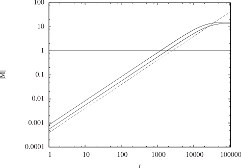
Figure 2: The time-dependent velocity field of a spherically symmetric accretion system is scaled as the Mach number, ${\mathrm{M}}$, and its time evolution is followed at $0.9r_{\mathrm{c}}$ (the upper full line) and $1.1r_{\mathrm{c}}$ (the lower full line). In the early stages of the evolution, both lines indicate a power-law dynamics, $|{\mathrm{M}}|\sim t$. The lower full line, pertaining to the dynamics in the subcritical region outside the sonic radius, overshoots the expected steady subsonic limit of the Bondi (1952) solution, and indicates the attainment of highly supersonic speeds, a fact that is clear from the way the solution crosses the sonic barrier at $|{\mathrm{M}}|=1$ (marked by the horizontal line in the plot). The lowermost dotted line is due to a toy function, used to test the correct exponent of the power law in the early stages of the evolution of $|{\mathrm{M}}|$. On later time scales the two full lines fall short of this power-law growth and converge towards an unexpectedly large limiting value of $|{\mathrm{M}}|\sim 10$.

A numerical exercise bears out the contention about how adversely the saddle point affects the dynamics. The $\log$–$\log$ graph shown in Figure 2 has been obtained by numerically integrating equations (1) and (2) by the finite-differencing technique. The integration has been performed under the flat initial conditions, $v=0$ and $\rho=10^{-21}{\mathrm{kg\,m^{-3}}}$ at $t=0$, for all values of $r$. Insofar as the purpose of the numerical study is to know the effects of nonlinearity in the dynamic evolution (not merely the perturbation), this initial condition is the most appropriate one. To appreciate this fact, we recall that the perturbation scheme on the velocity field is $v(r,t)=v_{0}(r)+v^{\prime}(r,t)$. Now, linearity holds under the requirement, $|v^{\prime}/v_{0}|\ll 1$. Once the initial velocity field is prescribed to be zero everywhere, i.e. $v(r,0)=0$, then from a perturbative perspective, this null initial condition can also be viewed as a global background state, $v_{0}(r)=0$. Thereafter, any arbitrarily small perturbation, $v^{\prime}$, on this zero initial state, will be of a fully nonlinear order, i.e. $v(r,t)=v^{\prime}(r,t)$. The growth of such a small time-dependent perturbation will become the actual dynamics of the global solutions, and this dynamics will be completely nonlinear.

In the numerics, the spherically symmetric flow is made to be driven by the Newtonian gravity of a star of mass, $M_{\odot}$. The polytropic index of the accreting gas is given as $n=1.51$, and the “ambient” conditions of the accreting gas are given by $c_{\mathrm{s}}(\infty)=10\,{\mathrm{km\,s^{-1}}}$ and $\rho_{\infty}=10^{-21}{\mathrm{kg\,m^{-3}}}$. In terms of all these fixed parameters of the flow, the sonic radius is scaled as $r_{\mathrm{c}}=(n-1.5)GM_{\odot}/2nc_{\mathrm{s}}^{2}(\infty)$ (Chakrabarti, 1990; Frank et al., 2002). The velocity field is scaled as the Mach number, ${\mathrm{M}}$, which is effectively the bulk velocity measured locally in terms of the speed of sound. In accretion flows, the bulk velocity is conventionally assigned a negative sign Frank et al. (2002), and so we present the absolute value of the Mach number, $|{\mathrm{M}}|$, in Figure 2. The time evolution of $|{\mathrm{M}}|$ is observed at $0.9r_{\mathrm{c}}$ (inside the sonic radius) and $1.1r_{\mathrm{c}}$ (outside the sonic radius). The two full lines in Figure 2 suggest a linear growth on early time scales for the Mach number, i.e. $|{\mathrm{M}}|\sim t$, a feature that prevails over four orders of magnitude. On later time scales, both lines show a convergence of the velocity field towards a limiting value (${\mathrm{M}}\sim 10$), but this value is far greater than what is expected from the stationary Bondi (1952) profile of the velocity field (which, in the neighbourhood of the sonic radius, is ${\mathrm{M}}\simeq 1$). This feature is particularly curious for the lower full line (plotted for $r>r_{\mathrm{c}}$), which shows an attainment of supersonic velocity, when even for the transonic solution, the steady velocity field outside the sonic radius has to be subsonic. This aspect of the dynamics is connected to the instability that arises due to the saddle point in the Liénard system, and near the steady sonic radius, also shows that nonlinearly strong signals may overshoot the constraints imposed by the acoustic horizon (Mach and Malec, 2008). The ultimate convergence towards an unexpectedly large limiting value (${\mathrm{M}}\sim 10$) occurs because of the saturating effect of the orders of nonlinearity higher than the second. Studies of the hydraulic jump phenomenon have reported similar saturation of a nonlinearly growing instability in the vicinity of the critical point of the flow Volovik (2006); Ray and Bhattacharjee (2007b).

Figure 3: Under pressureless conditions in the inflow ($v<0$), imposed on equation (2), the slope of this logarithmic plot shows that in the early stages of the evolution, $-v$ varies linearly with $t$. Deviation from linear growth sets in later. The horizontal line at the top shows the free-fall value of the velocity field, $\sqrt{2G{M_{\odot}}/51{r_{\odot}}}$, at a fixed radius of $51r_{\odot}$. There is a convergence in the dynamics towards this limiting value, and this may be seen in contrast to the overshoot of the expected limit shown in Figure 2.

The purport of Figure 2 can be compared with the convergence exhibited by the time-evolving velocity field in a “pressureless” fluid approximation (Shu, 1991) towards the free-fall limiting velocity of $\sqrt{2G{M_{\odot}}/r}$, with $r=51r_{\odot}$ Roy and Ray (2007). This convergence is shown graphically in Figure 3, and should be seen alongside Figure 2 for contrast. The numerical convergence of the velocity, demonstrated by finite-differencing integration, is also in full agreement with the analytical treatment of the time evolution of the pressureless flow, carried out by the method of characteristics (Ray and Bhattacharjee, 2002; Roy and Ray, 2007). Equation (2), rendered simple by setting $P=0$, under the requirement of a pressureless field driven by Newtonian gravity, appears as

$$\frac{\partial v}{\partial t}+v\frac{\partial v}{\partial r}+\frac{GM}{r^{2}}=0,$$ (25)

and can be solved by the method of characteristics (Debnath, 1997). The characteristic solutions are obtained from

$$\frac{{\mathrm{d}}t}{1}=\frac{{\mathrm{d}}r}{v}=\frac{{\mathrm{d}}v}{-GM/r^{2}}.$$ (26)

First, solving the ${\mathrm{d}}v/{\mathrm{d}}r$ equation will give

$$\frac{v^{2}}{2}-\frac{GM}{r}=\frac{c^{2}}{2},$$ (27)

in which $c$ is an integration constant, coming from the spatial part of the characteristic equation. We use this result to solve the ${\mathrm{d}}r/{\mathrm{d}}t$ equation in equation (26), to get

$$\frac{2vr}{cr_{\mathrm{s}}}-\ln r-\ln\left(\frac{v}{c}+1\right)^{2}-\frac{2ct}{r_{\mathrm{s}}}={\tilde{c}},$$ (28)

with $\tilde{c}$ being another integration constant, and $r_{\mathrm{s}}$ being a length scale in the system, defined as $r_{\mathrm{s}}=2GM/c^{2}$. The general solution of equation (26) is given by the condition, $F({\tilde{c}})=c^{2}/2$, with $F$ being an arbitrary function, whose form is to be determined from the initial condition. So, making use of equations (27) and (28), we first write the general solution as

$$\frac{v^{2}}{2}-\frac{GM}{r}=F\left[\frac{2vr}{c{r_{\mathrm{s}}}}-\ln r-\ln\left(\frac{v}{c}+1\right)^{2}-\frac{2ct}{r_{\mathrm{s}}}\right],$$ (29)

to determine whose particular form, we then use the initial condition, $v=0$ at $t=0$ for all $r$. This gives us

$$\frac{v^{2}}{2}-\frac{GM}{r}=-\frac{GM}{r}\left(\frac{v}{c}+1\right)^{-2}\exp\left(\frac{2vr}{cr_{\mathrm{s}}}-\frac{2ct}{r_{\mathrm{s}}}\right),$$ (30)

from which we see that for $t\longrightarrow\infty$, the right hand side of equation (30) vanishes, and its left hand side implies a convergence of the velocity field towards its stationary free-fall limit, i.e. $v=\sqrt{2GM/r}$. Corresponding to the given initial condition, this is evidently the final stationary solution associated with the lowest possible total energy, and the temporal evolution selects this solution. To envisage the evolution, the pressureless system, with a uniform velocity of $v=0$ everywhere, suddenly has a gravity mechanism activated in its midst at $t=0$. This induces a potential, $-GM/r$, at all points in space. The system then starts evolving to restore itself to another stationary state, with the velocity increasing according to equation (30), so that for $t\longrightarrow\infty$, the total energy at all points, $(v^{2}/2)-(GM/r)=0$, remains the same as what it was at $t=0$. This selection mechanism is compatible with the Bondi (1952) criterion of a particular solution being chosen by the virtue of possessing the minimum energy.

So how is the expected convergence achieved in the pressureless fluid approximation, while there seems to be an overshoot of the Bondi (1952) limit by a very wide margin, when we accommodate the pressure effects in the momentum balance condition of the flow? Understanding of this question requires returning to the seminal work of Bondi (1952), in which he referred to some earlier works which had adopted the pressureless prescription, and had studied only the dynamical effects. Bondi (1952) himself adopted the opposite extreme of negligible dynamical effects but full pressure effects, as described by stationary flow equations. The difficulty arises when the dynamically evolving velocity field is nonlinearly coupled to the dynamically evolving density field, through the pressure effects and the continuity equation, as can be seen in equations (1) and (2). We contend that the instability shown by the Liénard system is connected to this nonlinear coupling of the two dynamic fields. More to the point, there will be no such Liénard system under the pressureless condition. Not to mention also that the stationary problem is not equipped to capture this nonlinear instability, and time-dependent linearization around stationary states is nearly as inadequate. Another interesting point in the complete dynamic-plus-pressure scenario is that the overshooting of the steady subsonic limit by the lower full line in Figure 2 becomes more pronounced as the polytropic index, $n$, gets closer to the adiabatic limit of $n=1.5$ (or equivalently, $\gamma=5/3$). Evidently, near this limit, the density field, $\rho$, fortified by a high power law, due to the polytropic prescription, $P=k\rho^{\gamma}$, robustly affects the dynamics of the momentum balance condition. So, coupling with the density field does serve to destabilize the velocity field, as it evolves dynamically.

A final important point bears discussion. The two coupled fields, $v(r,t)$ and $\rho(r,t)$, are described by equations (1) and (2), which are both first-order differential equations. This two-variable mathematical problem was reduced to a one-variable problem, by introducing a new variable, $f=\rho vr^{2}$. The entire perturbative study and all consequent analytical results, involve this new variable only, with the perturbed quantity on its stationary background being $f^{\prime}(r,t)$. The price of this one-variable convenience is a second-order differential equation, as can be seen from equation (7). While the analytical treatment in this work is based on the variable, $f(r,t)$, the numerics, however, has followed the growth of the perturbation by means of the field, $v(r,t)$ (scaled as the Mach number, as Figure 2 indicates). In spite of this apparent difference, there is actually no contradiction between the analytical methods and the numerics, because from equation (3), it is clear that $|v^{\prime}/v_{0}|\sim|f^{\prime}/f_{0}|$, to a linear order. A precise analysis, of the kind leading to equation (13), yields $|v^{\prime}/v_{0}|=(1-\sigma)|f^{\prime}/f_{0}|$. This linear scaling between $f^{\prime}$ and $v^{\prime}$ suggests that the unstable growth behaviour of the one will be faithfully captured by the other. We have chosen the variable, $v$ (scaled by the speed of sound), to numerically track the growth of the perturbation, because in accretion fluid mechanics, flow solutions are categorized in terms of how the bulk flow velocity measures up to the local speed of sound (e.g., transonic, subsonic, globally supersonic, etc.)

VII Concluding remarks

It will be well in order now to make some general remarks about our work, to put it in perspective. First, accretion being a fluid problem, is very much within the realm of nonlinear dynamics. Our work addresses the nonlinear aspects of the dynamics of an accretion process, by having recourse to the usual analytical tools of nonlinear dynamics. One salient outcome of the nonlinear approach is obtaining an acoustic metric, in spite of accommodating nonlinearity completely. This marks a significant departure from the linear treatment (small perturbation) of the problem. Another new result of this work is the discovery of a Liénard system (a nonlinear oscillator) in a very common and basic model of accretion. A noteworthy aspect of all these new results is that they have been extracted from a system that has been known to the astrophysical community for more than sixty years — a conservative, non-self-gravitating, compressible fluid inflow, driven by Newtonian-like external gravitational fields, with coupled density and velocity fields. It is a very simple system in essence, and yet it continues to offer novel insights.

Going by the form of the Liénard system derived here, it is easy to see that the number of equilibrium points will depend on the order of nonlinearity that we may wish to retain in the equation of the perturbation. In practice, however, the analytical task becomes formidable with the inclusion of every higher order of nonlinearity. Going up to the second order, an instability in real time appears undeniable, but then we must realize that this conclusion has been made regarding a purely inviscid and conservative flow. Real fluids have viscosity as another important physical factor to influence their dynamics. In fact, fluid flows are usually affected by both nonlinearity and viscosity, occasionally as competing effects, and apropos of this point, we note that for a linearized radial perturbation in spherically symmetric inflows, viscosity helps in decaying the amplitude of the standing waves on globally subsonic solutions (Ray, 2003). So the instability that arises because of nonlinearity can very well be tempered by viscosity in the flow (Stellingwerf and Buff, 1978). Closely related to viscous dissipation, the stability of spherically symmetric accretion is expected to be affected by turbulence as well (Ray and Bhattacharjee, 2005).

A suitable mechanism that favours stability may be found in accretion onto black holes, where the coupling of the flow with the geometry of space-time acts in the manner of a dissipating effect. General relativistic effects have been known to enhance the stability of the flow (Naskar et al., 2007). And the stability of fluids may also be studied by constraining a perturbation to behave like a travelling wave (Petterson et al., 1980; Ray and Bhattacharjee, 2007b; Naskar et al., 2007; Sarkar et al., 2014). At times, we encounter the surprising situation of a fluid flow being stable under one type of perturbation, but unstable under the effect of another (Ray and Bhattacharjee, 2007b). Formally involving nonlinearity, all these features merit a close examination.