Abstract

We report on our search for genetically related asteroids amongst the near-Earth object (NEO) population — families of NEOs akin to the well known main belt asteroid families. We used the technique proposed by Fu et al. (2005) supplemented with a detailed analysis of the statistical significance of the detected clusters. Their significance was assessed by comparison to identical searches performed on 1,000 ‘fuzzy-real’ NEO orbit distribution models that we developed for this purpose. The family-free ‘fuzzy-real’ NEO models maintain both the micro and macro distribution of 5 orbital elements (ignoring the mean anomaly). Three clusters were identified that contain four or more NEOs but none of them are statistically significant at $\geq 3\sigma$. The most statistically significant cluster at the $\sim 2\sigma$ level contains 4 objects with $H<20$ and all members have long observational arcs and concomitant good orbital elements. Despite the low statistical significance we performed several other tests on the cluster to determine if it is likely a genetic family. The tests included examining the cluster’s taxonomy, size-frequency distribution, consistency with a family-forming event during tidal disruption in a close approach to Mars, and whether it is detectable in a proper element cluster search. None of these tests exclude the possibility that the cluster is a family but neither do they confirm the hypothesis. We conclude that we have not identified any NEO families.

Key Words: NEAR-EARTH OBJECTS, ASTEROIDS, DYNAMICS

1 Introduction

We report here on our null search for a statistically significant cluster of genetically related near-Earth objects (NEO). The identification of such a NEO ‘family’ would enable further research into the physical characteristics of NEOs as was the case with the identification of asteroid families in the main belt, Jupiter Trojan and Trans-Neptunian minor planet populations. The physical characteristics of the ensemble of NEO family members — taxonomic and mineralogical types, sizes, rotation periods, shapes, pole orientations, existence of satellites, etc.— would lead to a better understanding of their morphology and the mechanisms affecting their dynamical and collisional evolution. If the family members have a small minimum orbital intersection distance (MOID) with the Earth (or any other planet) their presence on a sub-set of dangerous orbits will increase the total impact probability over what is currently understood because the enhancement in orbit element phase space is not incorporated into contemporary NEO models.

In one sense there are already some known NEO families since associations have been proposed between several meteor showers and their presumed parent body NEOs (both asteroids and comets, e.g. Sekanina, 1973; Porubčan et al., 2004). The most known and well-accepted is the connection between the unusual B-type NEO (3200) Phaethon and the Geminid meteor complex Ohtsuka et al. (2008). However, the associations between meteors and NEOs are not families in the traditional undestanding. The known asteroid families are produced through the catastrophic disruption of a parent asteroid in a severe impact with another asteroid. The discovery of genetically related pairs of asteroids in the main belt (e.g. Vokrouhlický & Nesvorný, 2008) suggests that other mechanisms may produce asteroid families such as the spin-up and rotational fission of rapidly rotating objects or the splitting of unstable binary asteroids. Meteoroids are the small-end tail of those family creation mechanisms but can also be produced through surface ejection driven by the volatilization of sub-surface ices on comets or ‘active asteroids’. While no formal distinction exists between the meteor ‘families’ and the asteroid families the size ratio between the largest and second largest fragments nicely divides the samples and creation mechanisms.

No NEO families have been identified and confirmed. Drummond (2000) suggested that there were many ‘associations’ in the NEO population but Fu et al. (2005) showed that all of them were likely chance alignments of their orbits. The dearth of NEO families is in contrast to the more than 50 families known in the main belt (e.g. Nesvorný et al., 2005). Indeed, Hirayama (1918) proposed the existence of main belt asteroid families when there were only 790 known main belt asteroids while there are now more than 7,500 known NEOs.

Asteroid families are typically identified by the similarity of the family member’s orbital elements. Several metrics have been developed to quantify the orbital similarity (e.g. Southworth & Hawkins, 1963; Valsecchi et al., 1999; Jopek et al., 2008; Vokrouhlický & Nesvorný, 2008). The best known is the Southworth-Hawkins D-criterion ($D_{SH}$; Southworth & Hawkins, 1963) that was developed and used to search for parent comets of meteor streams and to link meteor streams with NEOs (e.g. Gajdoš & Porubčan, 2005; Ohtsuka et al., 2008).

It is important to keep in mind that simply identifying members within a population with similar orbital elements does not mean that they are actually a genetically related family. i.e. that they do not necessarily derive from a single parent object. As the number of objects in the population increases there is a corresponding increase in the likelihood that chance associations will mimic families and extra care must be taken to establish a proposed family’s statistical significance.

The major difference between the ability to identify families in the NEO and main belt populations is that the orbits of asteroids in the main belt are stable on timescales comparable to the age of solar system. Their long term stability allows the calculation of most objects’ proper elements (e.g. Knežević et al., 2002), essentially time-averaged orbital elements, that are better suited to the identification of similar orbits that are the hallmarks of asteroid families. Furthermore, the non-gravitational evolution of the main belt asteroids’ orbits is slow under the influence of the Yarkovsky effect (e.g. Vokrouhlický et al., 2006a) so that they occupy the same orbital element phase space for long periods of time.

The main belt families identified by the similarity in their orbit elements range in age from millions to billions of years. Spectroscopic campaigns have confirmed that the members of older families typically share the same spectral type; as expected if they all derive from the same parent body and/or are covered by similar regolith during the family formation event (e.g. Cellino et al., 2002; Ivezic̀ et al., 2002a). Near Earth objects on the other hand reside in a turbulent dynamical environment with average lifetimes of $\sim 10^{6}$ yr under the strong gravitational influence of the terrestrial planets and Jupiter (e.g. Morbidelli et al., 2002; Gladman et al., 1997). Thus, the calculation of NEO proper elements is difficult because they may cross the orbits of the planets during their time evolution (Gronchi & Milani, 2001). The resulting NEO proper elements are only valid for the time between their close encounters with the planets and when mean motion resonances of low order with the planets do not occur.

The search for similar orbits amongst the NEO population using only the osculating elements is even more limited in the time frame over which the orbits maintain their coherence (Pauls & Gladman, 2005). Furthermore, the non-gravitational accelerations acting on NEOs are generally much stronger than those acting on the more distant asteroids of the solar system. Thus, if a NEO family exists it will only be possible to identify it for a short time period after its creation as its members rapidly disperse.

NEO families might form by several imaginable methods (Fu et al., 2005):

• spontaneous disruption (e.g. YORP spin-up, internal thermal stresses)

• tidal disruption during close approach to a planet

• intra-NEO collisions

• collision with a smaller main belt asteroid

It is difficult or impossible to assign a likelihood to the different formation mechanisms. While 11% of comets spontaneously disrupt (e.g. Massi & Foglia, 2009) as they enter the inner solar system $(1.0AU<q\leq 1.5AU)$, presumably due to thermal stresses induced by approaching the Sun, the NEOs have typically resided in the terrestrial planet zone for long periods of time and many orbital periods. They are thus unlikely to disrupt by this mechanism. On the other hand, simulations suggest that the YORP thermal torque can increase an asteroid’s spin rate to the point where it spontaneously sheds material and some of this material may be ejected faster than the parent body’s escape speed (e.g. Walsh & Richardson, 2006; Pravec et al., 2010; Jacobson & Scheeres, 2011). If the process is repeated multiple times over a short time span it might be possible to create an asteroid family in this manner. Families created in this way might be distinguished by their rotation rates, mass ratios, or pole orientations of their members.

Tidal disruption of NEOs may occur when they pass close to a planet (e.g. Richardson et al., 1998; Walsh & Richardson, 2006, 2008) as occurred in the production of the family of objects associated with Comet Shoemaker-Levy-9 (Sekanina et al., 1994). While the tidal disruption of asteroids has been simulated under a variety of conditions (e.g., spin rate, pole orientation, closest approach distance, encounter speed), there is no estimate of how many tidal disruptions actually occur.

The likelihood of forming NEO families with the third mechanism is probably relatively small, since the space number-density of NEOs is very small compared to the space number-density of main belt asteroids (Bottke et al., 1996).

Perhaps the most likely formation mechanism for a NEO family is a collision between the NEO and a smaller main belt asteroid (Bottke et al., 1996). Many NEOs remain on orbits with aphelia in or beyond the main belt where they are typically slower than other asteroids at the same distance and therefore suffer higher speed collisions compared to those between two main belt asteroids at the same heliocentric distance. Thus, smaller projectiles could be effective impactors at catastrophically disrupting a NEO.

In summary, NEO families will provide to the opportunity of exploring the physics of asteroid disruptions at different scales and for different reasons than those observed in the main belt.

2 Method

We searched for families in the NEO population using the method proposed by Fu et al. (2005). The technique identifies subsets of objects with similar orbits within a population. We used their osculating elements, because of the problems involved in calculating NEO proper elements. We are thus limited to identifying NEO families that have formed relatively recently though this is not really a problem because 1) NEO dynamical lifetimes are on the order of a million years and 2) young families are interesting.

We used the Southworth-Hawkins $D_{SH}$ criteria (§2.1) to quantify the similarity between two orbits. It could be argued that other criteria would yield better results but this criteria has been well tested and forms the basis of the Fu et al. (2005) technique. A set of NEOs that all have mutual $D_{SH}$ criteria below a threshold $D_{cluster}$ is considered a ‘cluster’. The technique allows for and favors sub-clustering within the cluster under the assumption that there could be a tight ‘core’ within a cluster surrounded by a looser assemblage of related objects. We used the Minor Planet Center (MPC) mpcorb.dat orbit element data set that contained 7,563 NEOs as of March 2011 (through 2011 DW ). The technique is described in detail below.

The real difficulty in identifying NEO families is not the identification of the clusters but in establishing their statistical significance. Indeed, as shown by Fu et al. (2005) for NEOs and Pauls & Gladman (2005) for fireballs, it is surprisingly difficult to prove that similar orbits are statistically significant within a population. We first tested our method on synthetic family-free NEO orbit models but then developed more realistic family-free NEO models derived from the known NEO population. We used multiple instances of the family-free NEO models to establish the statistical significance of our NEO clusters.

2.1 The Southworth-Hawkins $D$-criterion

The Southworth-Hawkins $D_{SH}$ metric quantifies the similarity of two orbits using five orbital elements (Southworth & Hawkins, 1963). We use the $D_{SH}$ metric in its original form because it has an established pedigree (e.g. searching for parent comets of meteor streams) that has been used to successfully identify members of known meteor streams (Southworth & Hawkins, 1963; Sekanina, 1970) and main belt asteroid families (Lindblad & Southworth, 1971).

The $D_{SH}$ metric between two orbits denoted with subscripts $m$ and $n$ is defined by:

$$D_{SH}=\sqrt{{d_{1}}^{2}+{d_{2}}^{2}+{d_{3}}^{2}+{d_{4}}^{2}},$$ (1)

with

$$d_{1} = \frac{q_{m}-q_{n}}{AU},$$ (2)

$$d_{2} = e_{m}-e_{n},$$ (3)

$$d_{3} = 2\sin{(I/2)},$$ (4)

$$d_{4} = (e_{m}+e_{n})\sin{(\Pi/2)}$$ (5)

$$I = \arccos{\left[\cos{i_{m}}\cos{i_{n}}+\sin{i_{m}}\sin{i_{n}}\cos{(\Omega_{m}-\Omega_{n})}\right]},$$ (6)

$$\Pi = (\omega_{m}-\omega_{n})\pm 2\arcsin{\left[\cos{\frac{i_{m}+i_{n}}{2}}\sin{\frac{\Omega_{m}-\Omega_{n}}{2}}\sec{\frac{I}{2}}\right]},$$ (7)

where $q=a(1-e)$ is the perihelion distance, a is the semi-major axis, e is the eccentricity, i the inclination, $\Omega$ is the longitude of the ascending node and $\omega$ is the argument of perihelion. I represents the angle between the poles of the two orbits and $\Pi$ represents the angle between their perihelia directions (Drummond, 2000). Use the positive sign for the $\arcsin$ term in eq. 7 when $|\Omega_{m}-\Omega_{n}|\leq 180^{\circ}$ and the negative sign otherwise.

2.2 Identifying clusters in orbital element space

We adopted the cluster identification method developed by Fu et al. (2005) that in turn incorporated the techniques described by Drummond (2000). A ‘cluster’ is a grouping of objects with mutually similar orbits whereas we will reserve the term ‘family’ for a cluster with high statistical significance that contains members that are likely genetically related. Fu et al. (2005) showed in limited testing that the method is capable of identifying synthetic NEO families with minimal contamination.

We grouped objects into clusters based on the values of 4 parameters that are described in greater detail below:

• $D_{cluster}$: The maximum $D_{SH}$ between any pair of objects in a cluster.

• $D_{pair}$: The maximum $D_{SH}$ between ‘tight’ pairs in a cluster.

• $SCR_{min}$: The minimum String length to Cluster size Ratio.

• $PF_{min}$: The minimum fraction of pairs of asteroids in the cluster with $D_{SH}<D_{pair}$.

We identified candidate clusters as sets of $N$ objects with mutual $D_{SH}<D_{cluster}$. Within each candidate cluster we then identified all pairs ($n$) of asteroids with $D_{SH}<D_{pair}$. The pair fraction $PF$ is the number of detected pairs divided by the number of all possible pairs in the cluster ($PF=n/\frac{N(N-1)}{2}$) and we required that all our clusters satisfy $PF>PF_{min}$. Then, within each candidate cluster we determined the maximum string length $L$ — the maximum number of objects that are connected in a continuous pair-wise fashion such that each sequential pair in the string satisfies $D_{SH}<D_{pair}$. The $SCR$ is the ratio of the number of objects in the string to the number of objects in the cluster, $SCR=L/N$, and our final set of clusters all satisfy $SCR>SCR_{min}$. Note that a string must contain more than two objects.

The goal of our selection criteria is to identify tight clusters of objects in orbital element space but the $PF$ and $SCR$ cuts recognize that as NEOs undergo rapid dynamical and non-gravitational evolution some of the members may evolve quickly onto different orbits. The pair and string searches allow for a tight ‘core’ of objects with a periphery of other objects.

2.3 Selecting thresholds for the cluster identification algorithm

While it is simple to verify that our algorithm can identify objects in clusters with similar orbital elements it is not trivial to select the four threshold parameters ($D_{cluster}$, $D_{pair}$, $SCR_{min}$, $PF_{min}$) to maximize the cluster detection efficiency while minimizing the contamination by false positives. This required a family-free NEO orbit distribution model that also incorporated the observational selection effects typical of the asteroid surveys contributing the current NEO inventory. The selection effects are important because e.g. they favor the discovery of objects on Earth-like orbits and therefore increase the orbital element phase-space density of known objects on these types of orbits.

2.3.1 Synthetic family-free NEO model

To generate our synthetic family-free NEO model we started with the set of NEOs from the Synthetic Solar System Model (S3M; Grav et al., 2011). The S3M includes over 11 million objects ranging from those that orbit the Sun entirely interior to the Earth’s orbit to the most distant reaches of the solar system. The 268,896 NEOs with absolute magnitude $H<25.0$ in the S3M were generated in accordance with the $(a,e,i)$ orbital element residence-time distribution of the Bottke et al. (2002) NEO model. The model does not include any NEO families.

To model the observational selection effects on the S3M NEO population we performed a long-term survey simulation using the Pan-STARRS Moving Object Processing System (Denneau et al., 2007). MOPS was developed to process source detection data from Pan-STARRS (Kaiser et al., 2010) but also incorporates real-time processing of synthetic detections to monitor the system’s performance. Thus, it can be also used as a pure survey simulator.

In an ecliptic longitude ($\lambda_{0}$) and latitude ($\beta$) system centered on the opposition point $(\lambda_{0},\beta)=(0^{\circ},0^{\circ})$ the MOPS simulated survey region is broken into two regions covering about 5,500 deg²: 1) the opposition region with $|\lambda_{0}|<30^{\circ}$ and $|\beta|<40^{\circ}$ and 2) two ‘sweet spots’ with $|\beta|<10^{\circ}$ and $60^{\circ}<|\lambda_{0}|<90^{\circ}$.

MOPS uses a full $N$-body ephemeris determination to calculate the exact ($RA$, $Dec$) of every NEO in each synthetic field and then degrades the astrometry to the realized PS1 astrometric error level of 0.1^′′ (Milani et al. (2012) have shown that PS1 achieves $\sim 0.13^{\prime\prime}$ absolute astrometric error). The photometry for each object is degraded in a S/N-dependent manner such that as S/N$\rightarrow$5 the magnitude error approaches $\sim$0.1 mag. MOPS then makes a cut at S/N=5 to simulate the statistical loss of detections near the PS1 system’s limiting magnitude¹ of $R\sim$22.7. Each field is observed twice each night within $\sim$15 minutes to allow the formation of tracklets, pairs of detections at nearly the same spatial location, that might represent the same solar system object. Fields are re-observed 3 times per lunation (simulated weather permitting) and tracklets are linked across nights to form tracks that are then tested for consistency using an initial orbit determination (IOD).

Detections in tracks with small astrometric residuals in the IOD are subsequently differentially corrected to obtain a final orbit. Our four-year MOPS survey simulation on the S3M NEO population yielded 8,020 derived objects (synthetic discoveries). Fig. 1 shows that the derived synthetic NEOs are a rough match to the known NEOs. Thus, our NEO survey simulation yields a set of synthetic NEOs that are a proxy for the known population including their observational selection effects (Jedicke et al., 2002). Pan-STARRS is currently operating a single prototype telescope on Haleakala, Hawaii, known as PS1.

2.3.2 Cluster identification in the synthetic NEO model

With a large amount of computing time we could identify the set of clusters detectable in the real NEO population for all possible combinations of the four thresholds — $D_{cluster}$, $D_{pair}$, $SCR_{min}$ and $PR_{min}$. But this is impractical because we will also need to run orders of magnitude more tests to establish the detected clusters’ statistical significance. We were guided in our selection of the thresholds by previous work, our own experience, and testing the algorithm on the synthetic NEO model.

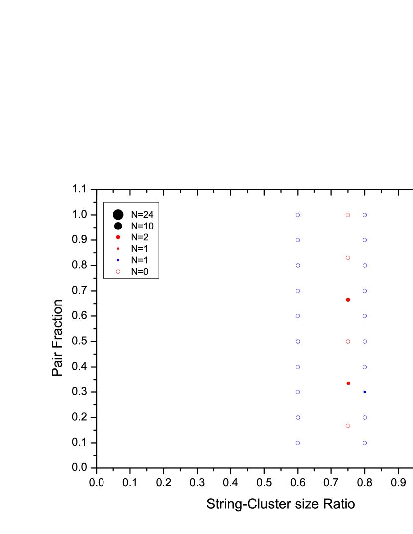
Figure 2: : Pair fraction ($PF$) vs. String to Cluster size Ratio ($SCR$) for false clusters detected in the family-free synthetic NEO model when $D_{cluster}=0.060$ and $D_{pair}=0.058$. The area of the filled circles is proportional to the number of false clusters at each $PF$-$SCR$ combination. Black circles represent clusters with 3 members, red is for clusters with 4 members, and blue represents clusters with $\geq$5 members. Empty black, red and blue circles represent the quantized possible values for 3, 4 and $\geq$5 member clusters respectively. It is impossible to have the combinations of $PF$ and $SCR$ on the left side of the figure.

Fig. 2 shows the results of the cluster identification method applied to the family-free synthetic NEO model using $D_{cluster}=0.060$ and $D_{pair}=0.058$ without any cuts on $SCR$ and $PF$. Even though our $D_{SH}$ thresholds are already considerably tighter than those proposed by Fu et al. (2005) we still identify many false clusters containing 3 members. We even identify one false 5-member cluster with $SCR=0.8$ and $PF=0.3$! However, the number of false clusters drops quickly with the number of cluster members (42 triplets, seven 4-member clusters and only one 5-member cluster). As the synthetic model is a good representation of the real NEO population we expect roughly the same number of false clusters amongst the real NEOs when we use the same $D_{cluster}$ - $D_{pair}$ cuts. Thus, even though we will explore the full range of tighter thresholds on the $D_{cluster}$ and $D_{pair}$ values as described below, based on Fig. 2 we will use $SCR_{min}=0.75$ and $PF_{min}=0.5$ to identify clusters containing $\geq 4$ members and not inspect the clusters containing NEO pairs and triplets. Establishing the smaller clusters’ statistical significance will be difficult or impossible using the techniques developed here.

In the following section §2.4 we will use the thresholds derived here to identify real NEO families for detailed analysis. However, when we measure the statistical significance of those NEO families in §3 we will abandon the synthetic model in favor of a more realistic one — but the more realistic model must be created using the thresholds derived here.

2.4 NEO clusters in the real population

We identified three clusters of four or more members in the real NEO population from the mpcorb.dat database. (We will ignore the 13 triplets and 243 pairs identified with the same cuts.) The members’ orbital elements and other physical parameters are provided in Tables 1 and 2. The three clusters are labelled C1, C2 and C3, and have 4, 6 and 5 members respectively. The absolute magnitudes of the cluster members spans $18.5<H<29.5$ corresponding to diameters ranging from several meters up to several hundreds of meters depending on the choice of albedo.

The total number of $\geq 4$ member clusters identified in the real data should be compared to the 0 $\geq 4$ member clusters identified in the family-free synthetic data with $SCR_{min}=0.75$ and $PF_{min}=0.5$ (see Fig. 2). The disparity in the number of $\geq 4$-member clusters could be due to the presence of real NEO families but we will argue below that it is due to the lack of fidelity in the synthetic NEO model — we find that the synthetic NEO model must be exquisitely matched to the real NEO population in order to assess the statistical significance of the detected clusters.

The C1 cluster is the only one composed of objects with $H<20$ and, more importantly, the only one containing objects with orbital arcs longer than 100 days. The C1 cluster members’ orbital element uncertainties are typically 1-2 orders of magnitude lower than the other two clusters. All the C1 members belong to the Amor NEO sub-population so that they do not cross the Earth’s orbit. Indeed, the members of this cluster have a perihelion distance of $\sim 1.25$ AU implying that if the cluster is a genetic NEO family it has probably never approached close to the Earth or Venus. Considering the similarity of all 5 orbital elements the cluster must have formed relatively recently and it is unlikely that the cluster or its members could have approached the Earth and then evolved onto orbits that do not cross the Earth’s on a short time scale.

In contrast to the C1 cluster, the C2 and C3 clusters are composed of small objects with $H>21.1$ and $H>27.7$ respectively and include objects with orbital arcs sometimes spanning just several days. The short arc lengths yield large uncertainties on the orbital elements which in turn induce a large uncertainty in the C2 and C3 $D_{SH}$. The clusters thus illustrate how false associations can arise because of the orbit element uncertainties. The nominal orbits of the two clusters place them in the Apollo NEO sub-population with the C2 cluster lying close to the Amor-Apollo transition and the C3 cluster close to the Apollo-Aten transition. Their location near the transition regions is not a coincidence — these small objects were identified by NEO surveys only because their orbits bring them very close to Earth. The perihelion distance is $\sim 1.00$ AU for the members of the C2 cluster while the members of the C3 cluster are on very Earth-like orbits with $a\sim 1.00$ and $e<0.1$. Establishing the C2 and C3 clusters’ statistical significance would be difficult because observational selection effects are not well-characterized for objects in their size range and this induces a large uncertainty in the orbit and size-distribution models for small NEOs.

Given the problems with the C2 and C3 clusters we will concentrate on establishing the statistical significance of the C1 cluster. One method of doing so is to run the cluster finding algorithm on many instances of the synthetic family-free NEO model described in §2.3.1. If we identify $\leq 3$ false clusters of $\geq 4$ members in 1,000 realizations of the synthetic NEO model we could claim that C1 is statistically significant with $\geq 99.7$% or $\geq 3\sigma$ confidence. We did not employ this technique because of our concerns with the use of the $\sim 10$ year old Bottke et al. (2002) NEO model that underestimates the number of Amor-type NEOs like the members of the C1 cluster. There are currently 474 known Amors with $H<18$ (as of March 2011) compared to the Bottke et al. (2002) prediction of $310\pm 38$ — a $>4\sigma$ difference between the real and synthetic NEO populations. If the Bottke et al. (2002) NEO model underestimates the number of Amor-type NEOs then it would imply that we will overestimate the C1 cluster’s statistical significance. Furthermore, the synthetic NEO model relies on a survey simulation that was not intended to perfectly model real surveys and yields $\sim$6% more objects than the real NEO population with small but perhaps significant skewing in the synthetic orbital element distributions as shown in Fig. 1. We need a better synthetic NEO model as described in the next section.

2.4.1 Fuzzy real NEO models

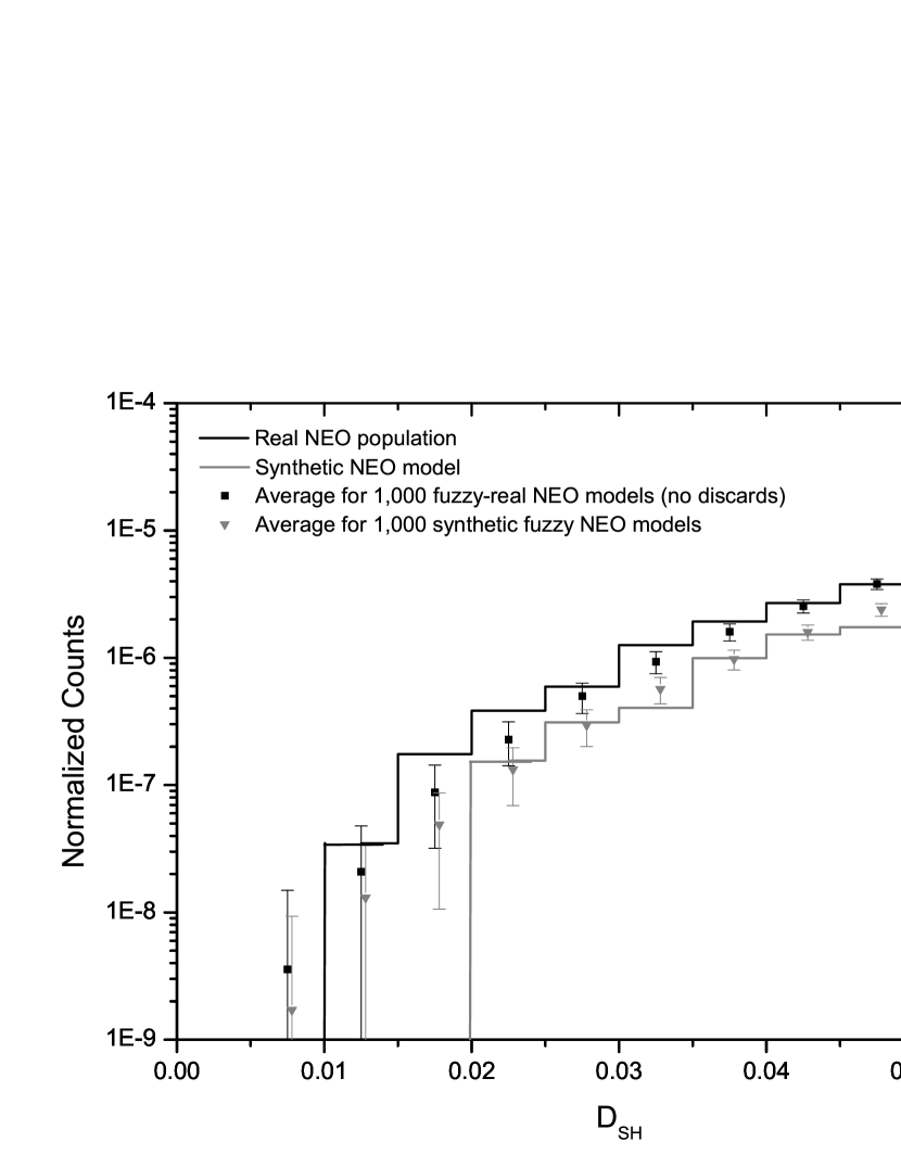
Figure 3: : $D_{SH}$ distribution of close NEO pairs normalized by the total number of possible pairs in each population. The solid black histogram represents the real NEO population while the black data points represent the average$\pm$RMS of 1,000 ‘fuzzy’ real NEO models (the ‘fuzzing’ technique is described in §2.4.1). The gray histogram represents the nominal synthetic NEO population while the grey data points represent the average$\pm$RMS of 1,000 ‘fuzzy’ synthetic NEO models.

The main problem with the Bottke et al. (2002) synthetic NEO model is illustrated in Fig. 3 — there is a huge discrepancy between the normalized $D_{SH}$ distributions for the closest pairs within the real and synthetic NEO populations. But establishing the statistical significance of our NEO clusters requires a large number of independent high-fidelity family-free NEO models that incorporate observational selection effects. Thus, we developed NEO models using a technique that i) maintains both the micro and macro distribution of 5 orbital elements (ignoring the mean anomaly) and ii) eliminates any possible real clusters.

Our solution was to ‘fuzz’ the orbital elements of each real NEO around its position in 5-dimensional orbital element space in a manner that maintained the local orbital element phase-space density and thereby preserves both the intrinsic NEO orbital element distribution and the observational selection effects. For each NEO ($k$) in the real population we identified its closest neighbor as the object with the smallest $D_{SH}\equiv D_{fuzz}$. We then generated a new ‘fuzzy’ synthetic orbit ($n$) that has $D_{SH}\leq D_{fuzz}$ with respect to the original orbit as described below.

If all the difference between the original and new orbit is due to a single orbital element (e.g. $\Delta a=a_{n}-a_{k}$) then we obtain $\Delta a$, $\Delta e$, $\Delta i$, $\Delta\omega$, and $\Delta\Omega$ from:

$$D_{fuzz} = \frac{(\Delta a)}{AU}(1-e)$$ (8)

$$= \Delta e\;\sqrt{1+(a/AU)^{2}}$$ (9)

$$= 2\;\sin(\Delta i/2)$$ (10)

$$= 2e\;\sin(\Delta\omega/2)$$ (11)

$$= \sqrt{{{d_{3}}^{\prime}}^{2}+{{d_{4}}^{\prime}}^{2}}$$ (12)

where

$${d_{3}}^{\prime} = 2\sin{(I_{\Delta\Omega}/2)},$$ (14)

$${d_{4}}^{\prime} = 2e\;\sin({\Pi_{\Delta\Omega}/2}),$$ (15)

and

$$I_{\Delta\Omega} = \arccos{\left[\cos^{2}{i}+\sin^{2}{i}\cos{\Delta\Omega}\right]}$$ (16)

$$\Pi_{\Delta\Omega} = 2\arcsin{\left[\cos{i}\sin\frac{\Delta\Omega}{2}\sec{\frac{I_{\Delta\Omega}}{2}}\right]}.$$ (17)

We then generated a ‘fuzzed’ orbit with $(a^{\prime},e^{\prime},i^{\prime},\omega^{\prime},\Omega^{\prime})$ where the elements $x^{\prime}$ were generated randomly within the range [$x-\Delta x,x+\Delta x$]. Finally, we calculated the $D_{\Delta}$ between the original and the fuzzed orbit and repeated the generation of the fuzzed orbit for the object until $D_{\Delta}<D_{fuzz}$. We also repeated the synthetic object generation if the new orbit was not a NEO (had perihelion $a^{\prime}(1-e^{\prime})>1.3$ AU), was hyperbolic (i.e. $e^{\prime}\geq 1$), or unphysical (e.g. $a^{\prime}\leq 0$, $e^{\prime}\leq 0$). We generated 1,000 instances of these ‘fuzzy-real NEO models’ to be used for establishing the statistical significance of our NEO clusters.

We tested the generation of the fuzzy-real NEO models by generating a series of models fuzzed by $D_{fuzz}^{\prime}=f_{fuzz}\;D_{fuzz}$ with $f_{fuzz}=0.0$, 0.2, 0.5, 1.0, 2.0, and 4.0 and verified that the models behave as expected and as $f_{fuzz}\rightarrow 0$ the generated model reproduces the input model exactly.

The remaining problem with the fuzzy-real NEO models is that if the real NEO population contains real families then so will the fuzzy-real NEO models. We needed to remove any real NEO families from the model first — but this is difficult to accomplish when there are no known real NEO families. Instead, we used our own cluster results agnostically with the assumption that it does not matter whether the clusters we identified are real or not, all that matters is how often the fuzzing process generates false clusters. Thus, i) using the cluster detection thresholds determined with the synthetic NEO population described in §2.3.1 we identified all clusters containing $\geq 3$ members and ii) treated the largest member of each cluster as any other NEO as described above but iii) fuzzed the orbits of the 18 smaller members of the clusters with $f_{fuzz}=10$. We needed to keep the 18 small objects in the model because they represent about 0.3% of the total known NEO population — about equal to the 3$\sigma$ contribution to the NEO model that we were attempting to measure. On the other hand we needed to keep them in roughly the correct location in the NEO orbit distribution.

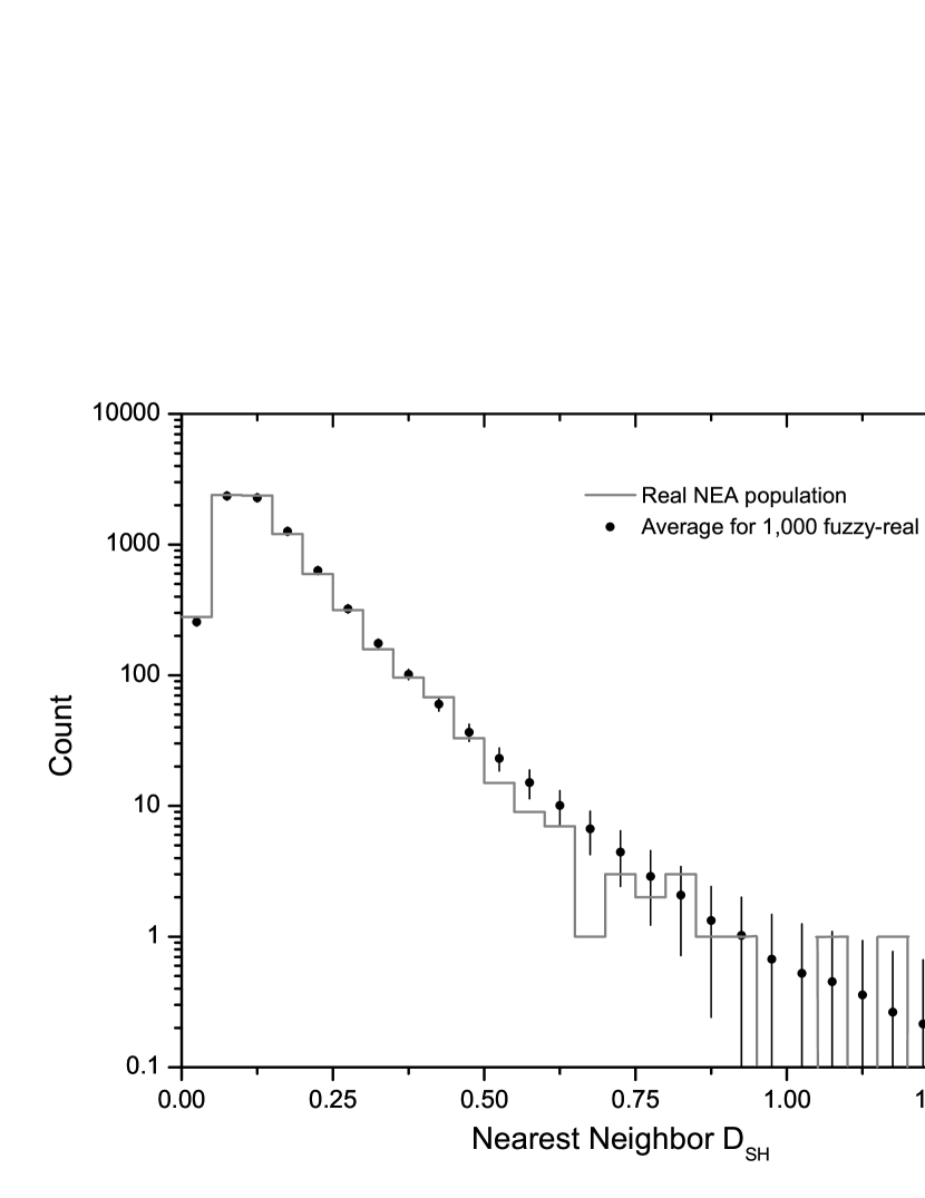
Figure 4: : $D_{SH}$ distribution for the closest neighboring objects in the real NEO population and the average$\pm$RMS for 1,000 fuzzy-real NEO models.

Fig. 1 shows that the fuzzy-real NEO models’ semi-major axis, eccentricity and inclination distributions match the known NEO population far better than the synthetic NEO model. Even more importantly, Figs. 3 and 4 show that the fuzzy-real NEO models preserve both the micro and macro $D_{SH}$ distributions (respectively) of the real NEO population that are critical to using the models to establish the statistical significance of the NEO clusters.

Note that the $D_{SH}$ distribution of the real NEOs is systematically slightly higher than the fuzzy-real NEO model at small $D_{SH}$ in Fig. 3. This would be the expected signature if there were real families in the real NEO population. The data point in the lowest $D_{SH}$ bins in Fig. 3 represent two separate pairs of NEOs. If these two pairs were real it would imply that they were statistically significant but it turned out that they were subsequently identified by the Minor Planet Center as corresponding to the same physical object. Thus, it is reassuring 1) that our fuzzy-real NEO model $D_{SH}$ distribution agrees well with the real NEOs and 2) that our technique successfully identified identical NEOs.

3 Results and discussion

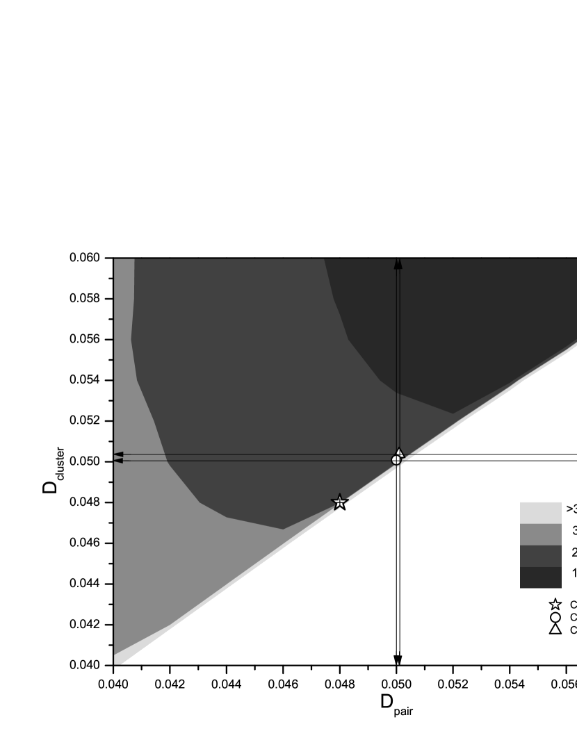
Figure 5: : Statistical significance of the C1, C2 and C3 clusters as a function of the $D_{cluster}$ and $D_{pair}$ thresholds with $SCR_{min}=0.75$ and $PF_{min}=0.5$. The shaded grey regions mark areas of 3-, 2-, and 1-$\sigma$ significance for clusters with $\geq 4$ members using the fuzzy-real NEO models (see text for details). The star, circle and triangle represent the most statistically significant location of the C1, C2 and C3 clusters respectively. The small black lines on the C1 data point represent the derived errors in $D_{cluster}$ and $D_{pair}$ due to the orbital element errors. The long vertical and horizontal lines through the C2 and C3 cluster’s data points represent the same errors for those clusters. The white region under the diagonal line is unphysical with $D_{cluster}<D_{pair}$.

The shaded regions in Fig. 5 show the results of running our cluster identification algorithm on the 1,000 family-free fuzzy-real NEO models described above. We searched for clusters containing $\geq 4$ members over the range of $D_{cluster}$–$D_{pair}$ space with $0.040\leq D_{cluster}\leq 0.060$ where $D_{pair}\leq D_{cluster}$ using fixed $SCR_{min}=0.75$ and $PF_{min}=0.5$ as described in §2.3.2. It is surprisingly easy to create NEO clusters with $\geq 4$ members. The shaded areas in the figure correspond to regions where we detected a total of a minimum of 3, 46 or 317 clusters in the 1,000 models. The regions correspond to 3-, 2- and 1$\sigma$ confidence levels on the detection of clusters in the real NEO population.

Fig. 5 also shows the location of our detected C1, C2 and C3 clusters in the real NEO population. The clusters can be identified over a limited range of $D_{cluster}$–$D_{pair}$ with the most statistically significant point typically having the smallest $D_{cluster}$ and $D_{pair}$. It may be surprising that the clusters are not identified in a broad fan extending upwards and to the right in the figure. The truncation in the region in which they are identifiable is due to the $SCR_{min}=0.75$ and $PF_{min}=0.5$ cuts — using looser values of $D_{cluster}$ and $D_{pair}$ allows the cluster to ‘absorb’ other nearby objects but these objects then typically drive the cluster’s $SCR$ and $PF$ values below the $SCR_{min}$ and $PF_{min}$ thresholds.

Fig. 5 shows that the C1 cluster is statistically significant at $\sim$2.0$\sigma$. The C2 and C3 clusters are likely even less significant based on their large $D_{cluster}$ and $D_{pair}$ error bars extending well into the insignificant region of the figure. It is important to remember that our calculated statistical significance of the NEO clusters hinges on the reliability of our fuzzy-real NEO models described in §2.4.1.

Given that all 4 C1 members are relatively large NEOs with $H<20$ we repeated the entire search for clusters using only those NEOs with $H<20$ and re-calculated their statistical significance. As expected, the statistical significance of the C1 cluster increases to about 3$\sigma$ because of the reduction in the total number of NEOs to $\sim 3100.$

While we have taken every precaution in developing our NEO models we understand that they have their limitations. For instance, the statistical significance of the NEO clusters increases/decreases if we ‘fuzz’ the model more/less ($f_{fuzz}>$/$<$1). We assume that the ‘natural’ value is $f_{fuzz}=1$ and use this value when quoting the statistical significance of our NEO clusters. In the remainder of this work we consider only the C1 cluster as a candidate NEO family.

3.1 Dismembering the C1 cluster

In this sub-section we perform several tests of the C1 cluster to determine if it is consistent with being a genetically related NEO family.

3.1.1 Provenance and taxonomy

Despite our minor caveats with the Bottke et al. (2002) NEO model described above it can still be used to estimate the probability that a NEO derives from one of their five NEO source regions. The C1 cluster falls in the NEO model bin with central $a=2.150$ AU, $e=0.425$ and $i=7.5^{\circ}$ for which objects have $\sim$35% probability of deriving from the $\nu_{6}$ region and a $\sim$63% chance of having evolved from the so called ‘Mars Crossing’ region. In other words, a nearly 100% probability of deriving from a source in the inner region of the main belt.

The inner region of the belt is dominated by S-class asteroids (e.g. Zellner, 1979) so it is a little surprising that SDSS spectrophotometry (from the 4^th Moving Object Catalog, MOC4; Ivezic̀ et al., 2002b) for the only available C1 cluster member, 2000 HW₂₃, is not S-like. We performed a simple linear interpolation and extrapolation of the 2000 HW₂₃ SDSS MOC4 5-band spectrophotometry and error bars to the SMASSII bands’ central wavelengths (Phase II of the Small Main-Belt Asteroid Spectroscopic Survey; Bus & Binzel, 2002). (The only extrapolation was from the real data point at 892 nm to the data point at 920 nm.)

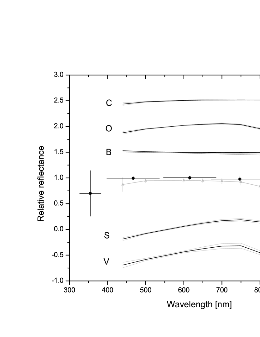
Figure 6: : Spectrophotometry of the C1 cluster’s largest member, 2000 HW₂₃, from the SDSS MOC4 by Ivezic̀ et al. (2002b) (black points) and the corresponding interpolated and extrapolated data points and error bars at the SMASSII filters’ central wavelengths Bus & Binzel (2002) (grey triangles and connecting lines). The synthetic SMASSII data points and lines are offset by -0.02 for clarity. The thin black curves and their adjacent grey curves represent the mean$\pm$RMS respectively of 5 asteroid taxonomic types from the SMASSII survey. All distributions have been corrected to solar colors and normalized to 1.0 at 550 nm. The relative reflectances of the C, O, B, S and V types are offset by +1.5, +1.0, +0.5, -1.0 and -1.5 respectively.

Even if at first glance the asteroid appears to be most similar to the O-type due to the dip in reflectivity at long wavelengths (see Fig. 6) a normalized $\chi^{2}$ fit of the 2000 HW₂₃ spectrophotometry to 26 major asteroid classes from $A$ through $X_{k}$ (from Bus & Binzel, 2002) suggests that it is most consistent with the unusual B-type, a subset of the larger C-complex. The O-type provides a close second best fit. In general, keeping in mind that the fit used data extrapolated from the SDSS MOC4 catalogue, 2000 HW₂₃ yields good fits with the different types in the C-complex — not the S-class that dominates the inner main belt.

The case for the C1 cluster being a legitimate family will be strengthened if the spectra of other C1 cluster members can be shown to be similar to 2000 HW₂₃ and belonging to the C-complex.

3.1.2 Size-frequency distribution

Under the assumption that C1 is a family we can estimate the slope of the family’s size-frequency distribution (SFD) assuming that the SFD is proportional to $10^{\alpha H}$. An unreasonable value of the slope would indicate that the cluster might not be a genetic family. Converting the observed C1 cluster member’s $H$ values into the true SFD requires the detection efficiency as a function of absolute magnitude, $\epsilon(H)$, for objects with C1-like orbits. We estimated $\epsilon(H)$ using the synthetic survey simulation described in §2.3.1 by dividing the number of derived objects with C1-like orbits by the number of objects in the input model. The survey simulation does a good enough job of reproducing the real NEO population for the purpose of estimating this efficiency and will not dominate the induced error on the measured SFD. We found a reasonable fit to the efficiency from the synthetic data using

$$\epsilon(H)={{\epsilon_{0}}\over{1+\exp[(H-L)/w]}}$$ (18)

with nominal values of $\epsilon_{0}=1.0$, $L$=20.0 and $w=0.76$. A maximum likelihood fit to the 4 C1 members’ $H$ distribution yields $\alpha=0.23^{+0.10}_{-0.08}$ where the error bars are statistical-only. The statistical errors on the fit are much larger than the systematic errors introduced by the uncertainty on the efficiency function parameters.

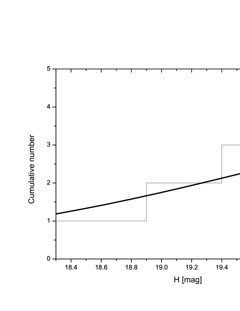
Figure 7: : Cumulative absolute magnitude distribution of the four C1 cluster members (grey). The thick black curve represents the product of the efficiency function (see text) with the result of the maximum likelihood fit to the SFD with $\alpha=0.23^{+0.10}_{-0.08}$.

The slope of the C1 cluster’s SFD (Fig. 7) is shallower but not inconsistent with the overall NEO population’s SFD of 0.35$\pm$0.02 measured by Bottke et al. (2002) for $H$<22 and it is surprisingly close to the value of 0.26$\pm$0.03 for H$\gtrsim$18 from Mainzer et al. (2011). Parker et al. (2008) measured the SFD for many main belt families and found that they can have complicated SFDs that can not be fit by a single power-law and that they have a wide range of slopes. The slope varies from 0.35 to 0.97 for single-slope families and from 0.10 to 0.62 at the faint end of the $H$ distribution for families with a broken power law SFD (i.e. $H$ values approaching those of the C1 cluster members). Furthermore, Richardson et al. (1998) suggests that tidally disrupted asteroid families have shallow SFDs. Thus, we can not use the SFD slope to exclude the hypothesis that the cluster is a family since the measured value is consistent with slopes of established families.

3.1.3 Backward orbit integrations & tidal disruption at Mars

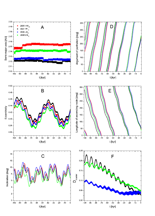
Figure 8: : Panels A-E: Backward evolution of the C1 cluster members’ orbital elements from the present ($t_{0}$) to 100 ky in the past. Panel F: $D_{cluster}$ evolution for the C1 cluster from $t_{0}$ to 100 ky in the past. $D_{cluster}$ was calculated with respect to 2000 HW₂₃ and therefore it does not appear on the panel. $D_{cluster}$ with respect to 2000 HW₂₃ does not differ significantly from the value calculated with respect to the average orbit of the C1 members.

If the C1 cluster is the remnant of a recently formed family then we expect that a backward integration of the 4 member’s nominal orbits would show a rapid convergence to a single orbit and the time frame for the convergence would indicate the time of the family’s formation (e.g. as observed in the Karin family; Nesvorný et al., 2006b). On the contrary, Fig. 8 shows that the nominal orbits are similar but undergo a gradual dispersal moving 100 ky into the past. i.e. they appear to have converged to their most similar orbits at the present time. The semi-major axis, eccentricity and inclinations of the members remain similar but the longitude of perihelion and ascending nodes gradually diverge. The effect is summarized in panel Fig. 8F showing the evolution of the cluster’s $D_{SH}$ with time. We note that two pairs of objects remain tight in their mutual $D_{SH}$ for the entire integration.

Given the apparent stability of the cluster members’ orbits we integrated all 4 nominal orbits backwards for 10 million years and found that they are exceptionally similar back to 1.5 Myr in the past. The mutual orbital stability is unusual for NEOs given that the numerical integrations showed numerous close encounters of all objects with Mars during this time. The lack of convergence of the nominal C1 members’ orbital elements suggests that they are not genetically linked. To firmly establish the statistical significance of the C1 cluster’s genetic relationship would require the generation of hundreds of clones of each C1 member and similarly generating clones for a large number of C1-like clusters.

Rather than explore that computationally challenging route we explored a few instances of the opposite question — is it possible that a family producing event in the recent past can reproduce the observed C1 cluster’s orbit and $D_{SH}$ distribution? We created 500 clones for each of the four C1 members where each clone is consistent with the available astrometry (the clones were generated using the covariance sampling technique in the OpenOrb orbit-computation package; Granvik et al., 2009). We integrated all the clones backwards in time for 100 ky and discovered that all of the objects suffered several close approaches with Mars and a large number of clones approached to within Mars’ Hill sphere. Since the C1 cluster is composed of Amor type NEOs we did not expect nor identify any close approaches to the Earth and Venus.

One 2000 HW₂₃ clone passed inside Mars’ Roche limit $\sim$70,800 years ago and is therefore a candidate for tidal disruptions (assuming that the parent body is a spherical fluid or rubble pile with a density $\rho$=1.95 g-cm^-3 like (25143) Itokawa (Abe et al., 2006), Mars’s Roche limit is $\sim$3.08 Mars radii). This result needs to be tempered with a comparison to the likelihood that any NEO will approach to within Mars’ Roche limit in the same time frame. We found that 5,070 of 8,133 known NEO’s nominal orbits approach Mars to within 1 Hill radii at least once during the last 100,000 years. Assuming that close approaches to within the Roche limit are as likely for clones of all NEOs (1 in 2000 C1 clones) then we might expect that about 2.5 of the known NEOs have actually approached to within Mars’ Roche limit and could be candidates for tidal disruption. Perhaps the C1 cluster’s hypothetical parent body is one of them and we will represent it as $\overline{\tt{2000\leavevmode\nobreak\ HW}_{23}}$ — the clone that made the closest approach to Mars mentioned above.

To study the properties of a family of objects created by tidal disruption by Mars we created twelve $\overline{\tt{2000\leavevmode\nobreak\ HW}_{23}}$ clones at the moment of its closest approach of 0.63 Mars Roche radii. The twelve secondary clones have $\Delta\vec{v_{x}}$, or $\Delta\vec{v_{y}}$, or $\Delta\vec{v_{z}}$ of $\pm$1 m-s^-1 and $\pm$5 m-s^-1 with respect to $\overline{\tt{2000\leavevmode\nobreak\ HW}_{23}}$. Simulations suggest that the tidal disruption process creates fragments with relative speeds of $<1$ m-s^-1 (Kevin Walsh, personal communication) so that our integrations will overestimate the spread in the orbital elements of tidally disrupted families. All 13 objects ($\overline{\tt{2000\leavevmode\nobreak\ HW}_{23}}$ and its 12 secondary clones) were integrated forward from the time of closest encounter to the present epoch with the same Bulirsch-Stoer integration routine and same time step as our other integrations.

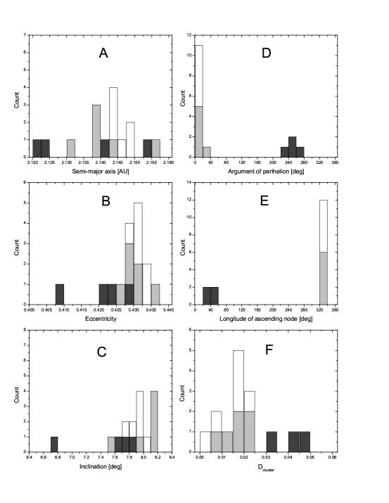
Figure 9: : Panels A-F: Orbital elements and $D_{cluster}$ distribution for the C1 custer members (dark grey) and two sets of 6 secondary $\overline{\tt{2000\leavevmode\nobreak\ HW}_{23}}$ clones (see text for description). The two sets of clones have $\Delta\vec{v_{x}}$, or $\Delta\vec{v_{y}}$, or $\Delta\vec{v_{z}}$ with respect to $\overline{\tt{2000\leavevmode\nobreak\ HW}_{23}}$ of $\pm$1 m-s^-1 (light grey) and $\pm$5 m-s^-1 (white) respectively at the time of closest Mars approach. There are only 3 values for the real C1 cluster because $D_{cluster}$ was calculated with respect to 2000 HW₂₃. The $D_{cluster}$ values for both sets of 6 secondary clones were calculated with respect to $\overline{\tt{2000\leavevmode\nobreak\ HW}_{23}}$ that was integrated simultaneously.

Panels A-E in Fig. 9 show that the values and ranges of $a$, $e$ and $i$ for the $\pm$1 m-s^-1 and $\pm$5 m-s^-1 groups of secondary clones are comparable to the values and ranges of the real C1 members. The ranges of $\Omega$ and $\omega$, ${\it i.e.}$ the spread of values within the two sets of $\overline{\tt{2000\leavevmode\nobreak\ HW}_{23}}$ clones and the 4 C1 cluster members, are also similar. The values of $\Omega$ and $\omega$ for the $\overline{\tt{2000\leavevmode\nobreak\ HW}_{23}}$ clones and the 4 C1 cluster members do not need to agree at the present time because the $\overline{\tt{2000\leavevmode\nobreak\ HW}_{23}}$ secondary clones were created from a single 2000 HW₂₃ clone whose orbit is slightly different from 2000 HW₂₃ due to the former’s deep approach to Mars (their semi-major axes differ by 0.05 AU). The difference between $\Omega$ and $\omega$ for the $\overline{\tt{2000\leavevmode\nobreak\ HW}_{23}}$ clones and the 4 C1 cluster members is thus due to their different precession rates that are sensitive to the initial values of semi-major axes (Murray & Dermott, 1999). Note that the actual C1 cluster member’s values show evidence of slightly more spreading than the $\overline{\tt{2000\leavevmode\nobreak\ HW}_{23}}$ secondary clones. Indeed, Fig. 9F shows that the distribution of $D_{cluster}$ for the $\overline{\tt{2000\leavevmode\nobreak\ HW}_{23}}$ secondary clones is also tighter than the C1 members. Both observations can be explained as being due to non-gravitational forces acting on the real objects over the course of the last $\sim$71 ky.

The distributions of orbital elements and $D_{cluster}$ in Fig. 9 suggests that the C1 cluster is consistent with an origin in the tidal disruption of an asteroid during a tidal disruption event with Mars 70,800 years ago. If true, the C1 cluster is a very young family. In a followup paper to this one we will show that the lifetime of tidally disrupted families created by Mars are as long as $\sim$1 Myr so if they exist it may not be surprising that we are beginning to detect them. Furthermore, if there is a tidally disrupted asteroid family in the NEO population it seems more likely to be a C-class asteroid and, ceteris paribus, will disrupt more easily since they have a lower bulk density than the S-class. (Richardson et al., 1998). Thus, it is interesting that one C1 member with spectrophotometry, 2000 HW₂₃, may be in the C-class (see §3.1.1).

3.1.4 Proper element cluster search

We also performed a cluster search with NEO proper elements (Gronchi & Milani, 2001). Since the C1 cluster was detected as a cluster in osculating element space it seems plausible that it should also be detectable in proper element space as described in the introduction. A complication arises because our cluster search algorithm uses a 5-element $D_{SH}$-criterion that incorporates the longitude of the ascending nodes and argument of perihelion (the $d_{3}$ and $d_{4}$ terms in eq. 1) while only the proper semi-major axis, eccentricity and inclination ($a_{p},e_{p},i_{p}$) can be calculated for asteroids. Thus, the $D_{SH}$ for clusters in proper element space, $D_{p}$, must be smaller than those found using the 5-element $D_{SH}$ with the osculating elements — $D_{cluster}=0.002$ compared to $D_{cluster}=0.040$ used for the osculating element cluster search.

The proper element cluster search revealed that the C1 cluster is not outstanding among NEO clusters. We identified a C1_p cluster in the proper element search that has 3 objects in common with the C1 cluster — 2000 HW₂₃, 2001 PF₁₄, and 2008 $LN_{16}$ — and there are 166 clusters with 5 or more members that are bound tighter than C1_p with $D_{p}$=0.018. The C1_p cluster contains two additional objects, 2002 RA₁₈₂ and 2004 TE₁₈, instead of 2006 JU₄₁. The osculating element $D_{SH}$  for 2004 TE₁₈ and 2002 RA₁₈₂ calculated with respect to 2000 HW₂₃ are 0.471 and 0.125, much too large to indicate an orbital similarity.

We found that the stability of the NEOs in the C1 and C1_p clusters is not unusual. We computed the MOID with all the planets from Mercury to Neptune during the secular evolution of 8,650 NEOs (NEODyS, 29/2/2012) according to the dynamical model used in the computation of the proper elements (Gronchi & Milani, 2001). Roughly 5% of all NEOs (429) do not cross the trajectory of any planet and $\sim 42$% of them (3,636) cross only Mars’ trajectory during their secular evolution.

The six asteroids in the C1 and C1_p clusters are of the latter type. Table 3 shows that all the cluster’s members remain far from both the Earth and Jupiter, the major NEO perturbers, during their entire secular cycles. Of the total 3,636 Mars crossing objects we find that

• $\sim$50% of them have $\min$(MOID_Earth) $\geq 0.1$ AU, and $\min$(MOID_Jupiter) $\geq 1$ AU,

• $\sim$16% of them have $\min$(MOID${}_{Earth})$ $\geq 0.2$ AU, and $\min$(MOID_Jupiter) $\geq 2$ AU.

Thus, even if some of them are affected by mean motion resonances it appears that many Mars crossing NEOs remain far from close encounters with, and are not affected by perturbations from, the Earth and Jupiter. A close approach with Mars must be very deep to cause a significant perturbation.

Thus, there are islands of long-term stability in the NEO orbital element phase space that might ‘collect’ NEOs in a manner that could mimic the appearance of a NEO family. The Bottke et al. (2002) NEO model can not accurately model these regions of stability because of its low resolution in the orbital element phase space, the relatively small number of objects that were originally used to map out the NEOs’ residence time probability distribution, and because it is restricted to just 3 of the 6 orbital elements.

4 Conclusions

We searched for genetic asteroid families in the NEO population using the method proposed by Fu et al. (2005) based on identifying clusters of objects with similar orbits. We enhanced the method’s utility by developing a technique for assessing the statistical significance of the identified clusters using 1,000 realistic family-free fuzzy-real NEO orbital element models. We created our NEO models by cloning members of the known NEO population in a natural way based on the ‘distance’ between each member and its nearest neighbor. The technique identified three clusters of four or more NEOs among the orbits in the mpcorb.dat data base. None of the clusters are statistically significant at $\geq 3\sigma$ and we conclude that there are as yet no identified families in the NEO population.

The most statistically significant cluster, C1, contains four objects all with $H<20$ and well-determined orbits with the largest member being asteroid 2000 HW₂₃. We performed several additional tests of the C1 cluster’s family veracity including checking the members’ taxonomic identification, their bias corrected size-frequency distribution, the possibility that they originated in a family-producing tidal disruption at Mars about 71k years in the past, and whether it is also identifiable as a cluster in proper element space. None of these tests exclude the possibility that C1 is a genetically related family but at the same time none of the tests provide sufficient evidence to elevate the cluster to family status.

The search for families amongst the NEO population is clearly not as straightforward as the same search amongst the main belt population. Special care must be taken when assessing the statistical significance of a purported NEO family especially with regard to accounting for observational selection effects in the NEO population. At the very least, mere similarity of the orbital elements as evidenced by the $D_{SH}$ criterion being less than an arbitrary and commonly used value like 0.2 is insufficient for deciding upon any genetic relationship between NEOs and, by extrapolation, between NEOs and meteors.

Name	$a$	$\Delta a$	$e$	$\Delta e$	$i$	$\Delta i$	$\omega$	$\Delta\omega$	$\Omega$	$\Delta\Omega$
	AU	$\times 10^{-7}$		$\times 10^{-6}$	deg	$\times 10^{-5}$	deg	$\times 10^{-4}$	deg	$\times 10^{-4}$
C1
2000 HW23	2.154	1	0.424	1	7.76	7	245	2	47	1
2006 JU41	2.123	5	0.429	2	7.61	8	236	3	52	2
2001 PF14	2.120	4	0.410	0.5	6.78	2	254	3	38	1
2008 LN16	2.141	5	0.421	0.2	7.82	2	261	4	36	2
C2
1999 YD	2.463	4000	0.593	70	1.38	12	62	0.2	10	20
2003 UW5	2.470	2$\times 10^{5}$	0.577	300	1.87	77	52	0.2	17	10
2008 UT5	2.279	2$\times 10^{5}$	0.555	400	1.61	91	33	0.1	38	10
2008 YW32	2.319	5$\times 10^{5}$	0.559	$10^{4}$	0.99	125	2	0.6	71	40
2007 YM	2.584	2$\times 10^{7}$	0.617	3$\times 10^{5}$	0.99	2$\times 10^{5}$	11	0.8	60	7$\times 10^{4}$
2005 WM3	2.674	3$\times 10^{5}$	0.620	400	1.23	56	190	0.3	240	10
C3
2008 EA9	1.059	342	0.080	38	0.42	23	336	30	129	30
2010 JW34	0.983	53	0.055	10	2.26	42	43	7	50	10
1991 VG	1.027	1	0.049	0.2	1.45	55	25	0.1	74	0.9
2009 BD	1.063	$10^{7}$	0.052	48	1.27	63	317	10	253	0.06
2006 RH120	1.033	$10^{7}$	0.024	21	0.60	9	10	600	51	0.4

Table 1: : Orbital elements for the members of 3 NEO clusters (C1, C2 & C3) with four or more members. Members of the clusters are listed in order of decreasing size. None of the clusters are statistically significant at $>3\sigma$. Data is from the JPL Small-Body Database Browser http://ssd.jpl.nasa.gov/sbdb.cgi.

Name	$H$	$D_{S}$	$D_{C}$	$D_{SH}$	$\Delta D_{SH}$
	mag	m	m		$\times 10^{-6}$
C1
2000 HW23	18.5	590	1,500	-	4
2006 JU41	19.3	410	1,100	0.041	6
2001 PF14	19.5	370	1,000	0.032	4
2008 LN16	19.9	311	803	0.048	4
C2
1999 YD	21.1	180	460	-	80
2003 UW5	24.3	40	110	0.051	3
2008 UT5	24.5	40	100	0.044	3
2008 YW32	25.2	30	70	0.049	10
2007 YM	26.2	180	40	0.052	1600
2005 WM3	27.7	8	20	0.026	170
C3
2008 EA9	27.7	8	22	0.039	4
2010 JW34	28.1	7	18	0.050	2
1991 VG	28.5	5	15	-	270
2009 BD	28.8	5	13	0.050	$10^{5}$
2006 RH120	29.5	3	9	0.049	$10^{5}$

Table 2: : Absolute magnitude ($H$), diameter ($D_{S}$ and $D_{C}$) and $D_{SH}$ for the members of 3 NEO clusters (C1, C2 & C3) with four or more members. Members of the clusters are listed in order of decreasing size. None of the clusters are statistically significant at $>3\sigma$. $D_{SH}$ and its uncertainty were calculated using the orbital elements and associated errors from www.jpl.org as shown in Table 1. The diameters $D_{S}$ and $D_{C}$ were calculated using albedos of $p_{V}=0.2$ and $p_{V}=0.03$ corresponding to the mean albedos of S and C class asteroids as reported by Mainzer et al. (2011).

name	$\min$(MOIDEarth)	$\min$(MOIDJupiter)
	AU	AU
2000 HW23	0.26782	2.16112
2001 PF14	0.27176	2.23225
2006 JU41	0.23183	2.18723
2008 LN16	0.26740	2.18886
2002 RA182	0.27768	2.16264
2004 TE18	0.26278	2.23812

Table 3: : Minimum MOID with the Earth and Jupiter for the NEOs in the C1 and C1_p clusters during the course of their secular evolution.

Figure 1: : Semi-major axis, eccentricity and inclination distributions of the real NEO population (solid line), the synthetic NEO model (dotted line) and our fuzzy-real NEO model (data points).

References

- (1)
- Abe et al. (2006) Abe, S., Mukai, T., Hirata, N., Barnouin-Jha, O. S., Cheng, A. F., Demura, H., Gaskell, R., Hashimoto, T., Hiraoka, K., Honda, T., Kubota, T., Matsuoka, M., Mizuno, T., Nakamura, R., Scheeres, D. & Yoshikawa, M. (2006), ‘Mass and Local Topography Measurements of Itokawa by Hayabusa’, Science 312, 1344–1349.
- Allen et al. (2005) Allen, D., Rodgers, C. T., Canterna, R., Hausel, E., Flores, E. & Smith, J. A. (2005), Fundamental Transformation Equations Between the u’g’r’i’z’ and UBVR Filter Systems, in ‘Bulletin of the American Astronomical Society’, Vol. 37, p. 1210.
- Bilir & Karaali (2005) Bilir, S. & Karaali, S. andTuncel, S. (2005), ‘Absolute magnitudes for late-type dwarf stars for Sloan photometry’, Astronomische Nachrichten 326, 321–331.
- Bottke et al. (2002) Bottke, W. F., Morbidelli, A., Jedicke, R., Petit, J. M., Levison, H. F., Michel, P. & Metcalfe, T. S. (2002), ‘Debiased Orbital and Absolute Magnitude Distribution of the Near-Earth Objects’, Icarus 156(2), 399–433.
- Bottke et al. (1996) Bottke, W. F., Nolan, M. C., Melosh, H. J., Vickery, A. M. & Greenberg, R. (1996), ‘Origin of spacewatch small Earth-approaching asteroids’, Icarus 256, 406–427.
- Bus & Binzel (2002) Bus, S. J. & Binzel, R. P. (2002), ‘Phase II of the Small Main-Belt Asteroid Spectroscopic SurveyA Feature-Based Taxonomy’, Icarus 158, 146–177.
- Cellino et al. (2002) Cellino, A., Bus, S. J., Doressoundiram, A. & Lazzaro, D. (2002), Spectroscopic properties of asteroid families, in W. Bottke, A. Cellino, P. Paolicchi & R. P. Binzel, eds, ‘Asteroids III’, University of Arizona Press, pp. 633–643.
- Denneau et al. (2007) Denneau, L., J., Kubica, J. & Jedicke, R. (2007), The Pan-STARRS Moving Object Pipeline, in R. A. Shaw, F. Hill, & D. J. Bell, eds, ‘Astronomical Data Analysis Software and Systems XVI ASP Conference Series #376’, Astronomical Data Analysis Software and Systems XVI ASP Conference Series #376, p. #257.
- Drummond (2000) Drummond, J. D. (2000), ‘The D-discriminant and Near-Earth Asteroid Streams’, Icarus 146(2), 453–475.
- Fu et al. (2005) Fu, H., Jedicke, R., Durda, D. D., Fevig, R. & Binzel, R. P. (2005), ‘Identifying near-Earth object families’, Icarus 178(2), 434–449.
- Gajdoš & Porubčan (2005) Gajdoš, S. & Porubčan, V. (2005), Bolide meteor streams, in ‘Dynamics of Populations of Planetary Systems, Proceedings of IAU Colloquium #197’, IAU Colloquium #197, pp. 393–398.
- Gladman et al. (1997) Gladman, B. J., Migliorini, F., Morbidelli, A., Zappala, V., Michel, P., Cellino, A., Froeschle, C., Levison, H. F., Bailey, M. & Duncan, M. (1997), ‘Dynamical lifetimes of objects injected into asteroid belt resonances’, Science 277, 197–201.
- Granvik et al. (2009) Granvik, M., Virtanen, J., Oszkiewicz, D. & Muinonen, K. (2009), ‘OpenOrb: Open-source asteroid orbit computation software including statistical ranging’, Meteoritics and Planetary Science 44, 1853–1861.
- Grav et al. (2011) Grav, T., Jedicke, R., Denneau, L., Chesley, S., Holman, M. J. & Spahr, T. B. (2011), ‘The Pan-STARRS Synthetic Solar System Model: A Tool for Testing and Efficiency Determination of the Moving Object Processing System’, Publications of the Astronomical Society of the Pacific 123, 423–447.
- Gronchi & Milani (2001) Gronchi, G. F. & Milani, A. (2001), ‘Proper Elements for Earth-Crossing Asteroids’, Icarus 152, 58–69.
- Hirayama (1918) Hirayama, H. (1918), ‘Groups of asteroids probably of common origin’, Astronomical Journal 31(743), 185–188.
- Ivezic̀ et al. (2002b) Ivezic̀, v., Juric̀, M., Lupton, R. & Tabachnik, S.AND Quinn, T. (2002b), SDSS MOC4, in J. Tyson & S. Wolff, eds, ‘Survey and Other Telescope Technologies and Discoveries’, Vol. 4836, Proceedings of the SPIE.
- Ivezic̀ et al. (2002a) Ivezic̀, v., Lupton, R. H., Juric̀, M., Tabachnik, S., Quinn, T., Gunn, J. E., Knapp, G. R., Rockosi, C. M. & Brinkmann, J. (2002a), ‘Color Confirmation of Asteroid Families’, The Astronomical Journal 124, 2943–2948.
- Jacobson & Scheeres (2011) Jacobson, S. A. & Scheeres, D. J. (2011), ‘Dynamics of rotationally fissioned asteroids: Source of observed small asteroid system’, Icarus 214, 161–178.
- Jedicke et al. (2002) Jedicke, R., Larsen, J. & Spahr, T. (2002), Observational Selection Effects in Asteroid Surveys , in W. Bottke, A. Cellino, P. Paolicchi & R. P. Binzel, eds, ‘Asteroids III’, University of Arizona Press, pp. 71–87.
- Jopek et al. (2008) Jopek, T. J., Rudawska, R. & Bartczak, P. (2008), ‘ Meteoroid Stream Searching: The Use of the Vectorial Elements’, Earth, Moon, and Planets 102(1), 73–78.
- Kaiser et al. (2010) Kaiser, N., Burgett, W., Chambers, K., Denneau, L., Heasley, J., Jedicke, R., Magnier, E., Morgan, J., Onaka, P. & Tonry, J. (2010), The Pan-STARRS wide-field optical/NIR imaging survey, in L. M. Stepp, R. Gilmozzi & H. J. Hall, eds, ‘Ground-based and Airborne Telescopes III’, Vol. 7733, Proceedings of the SPIE, pp. 77330E–77330E–14.
- Knežević et al. (2002) Knežević, Z., Lemaître, A. & Milani, A. (2002), The Determination of Asteroid Proper Elements, in W. Bottke, A. Cellino, P. Paolicchi & R. P. Binzel, eds, ‘Asteroids III’, University of Arizona Press, pp. 603–612.
- Lindblad & Southworth (1971) Lindblad, B. A. & Southworth, R. B. (1971), A Study of Asteroid Families and Streams by Computer Techniques, in T. Gehrels, ed., ‘Physical Studies of Minor Planets’, IAU Colloquium #12, p. 337.
- Mainzer et al. (2011) Mainzer, A., Grav, T., Bauer, J., Masiero, J., McMillan, R. S., Cutri, R. M., Walker, R., Wright, E., Eisenhardt, P., Tholen, D. J., Spahr, T., Jedicke, R., Denneau, L., DeBaun, E., Elsbury, D., Gautier, T., Gomillion, S., Hand, E., Mo, W., Watkins, J., Wilkins, A., Bryngelson, G. L., Del Pino Molina, A., Desai, S., Gómez Camus, M., Hidalgo, S. L., Konstantopoulos, I., Larsen, J. A., Maleszewski, C., Malkan, M. A., Mauduit, J.-C., Mullan, B. L., Olszewski, E. W., Pforr, J., Saro, A., Scotti, J. V. & Wasserman, L. H. (2011), ‘NEOWISE Observations of Near-Earth Objects: Preliminary Results’, Astrophysical Journal 743, 156.
- Massi & Foglia (2009) Massi, G. & Foglia, S. (2009), ‘Comet disruption: a statistical approach for the nearly isotropic comets’, Journal of the British Astronomical Association 119, 203–204.
- Milani et al. (2012) Milani, A., Knezevic, Z., Farnocchia, D., Bernardi, F., Jedicke, R., Denneau, L., Wainscoat, R. J., Burgett, W., Grav, T., Kaiser, N., Magnier, E. & Price, P. A. (2012), ‘Identification of known objects in solar system surveys’, eprint arXiv:1201.2587 .
- Morbidelli et al. (2002) Morbidelli, A., Bottke, J. W. F., Froeschlé, C. & Michel, P. (2002), Origin and Evolution of near-Earth Objects, in W. Bottke, A. Cellino, P. Paolicchi & R. P. Binzel, eds, ‘Asteroids III’, University of Arizona Press, pp. 409–422.
- Murray & Dermott (1999) Murray, C. D. & Dermott, S. F. (1999), Solar system dynamics, in ‘Solar system dynamics’, Cambridge University Press.
- Nesvorný et al. (2006b) Nesvorný, D., Enke, B. L., Bottke, W. F., Durda, D. D., Asphaug, E. & Richardson, D. C. (2006b), ‘Karin cluster formation by asteroid impact’, Icarus 183(2), 296–311.
- Nesvorný et al. (2005) Nesvorný, D., Jedicke, R., Whiteley, R. J. & Izvezic̀, Z. (2005), ‘Evidence for asteroid space weathering from the Sloan Digital Sky Survey ’, Icarus 173(1), 132–152.
- Ohtsuka et al. (2008) Ohtsuka, K., Arakida, H., Ito, T., Yoshikawa, M. & Asher, D. J. (2008), Apollo Asteroid 1999 YC: Another Large Member of the PGC?, in ‘71st Annual Meeting of the Meteoritical Society’, Annual Meeting of the Meteoritical Society #71, p. 5055.
- Parker et al. (2008) Parker, A., Ivezić, Ž., Jurić, M., Lupton, R., Sekora, M. D. & Kowalski, A. (2008), ‘The size distributions of asteroid families in the SDSS Moving Object Catalog 4’, Icarus 198, 138–155.
- Pauls & Gladman (2005) Pauls, A. & Gladman, B. (2005), ‘Decoherence time scales for ”meteoroid streams”’, Meteoritics and Planetary Science 40, 1241.
- Porubčan et al. (2004) Porubčan, V., Williams, I. P. & Kornoš, L. (2004), ‘Associations Between Asteroids and Meteoroid Streams’, Earth Moon and Planets 95, 697–712.
- Pravec et al. (2010) Pravec, P., Vokrouhlický, D., Polishook, D., Scheeres, D. J., Harris, A. W., Gal d, A., Vaduvescu, O., Pozo, F., Barr, A., Longa, P., Vachier, F., Colas, F., Pray, D. P., Pollock, J., Reichart, D., Ivarsen, K., Haislip, J., Lacluyze, A., Kušnirák, P., Henych, T., Marchis, F., Macomber, B., Jacobson, S. A., Krugly, Y. N., Sergeev, A. V. & Leroy, A. (2010), ‘Formation of asteroid pairs by rotational fission’, Nature 466, 1085–1088.
- Richardson et al. (1998) Richardson, D. C., Bottke, W. F. & Love, S. G. (1998), ‘Tidal Distortion and Disruption of Earth-Crossing Asteroids’, Icarus 134, 47–76.
- Sekanina (1970) Sekanina, Z. (1970), ‘Statistical Model of Meteor Streams. II. Major Showers’, Icarus 13, 475.
- Sekanina (1973) Sekanina, Z. (1973), ‘Statistical Model of Meteor Streams. III. Stream Search Among 19303 Radio Meteors’, Icarus 18, 253.
- Sekanina et al. (1994) Sekanina, Z., Chodas, P. & Yeomans, D. K. (1994), ‘Tidal disruption and the appearance of periodic comet Shoemaker-Levy 9’, Astronomy and Astrophysics 289, 607–636.
- Southworth & Hawkins (1963) Southworth, R. B. & Hawkins, G. S. (1963), ‘Statistics of meteor streams’, Smithsonian Contributions to Astrophysics 7, 261–285.
- Valsecchi et al. (1999) Valsecchi, G. B., Jopek, T. J. & Froeschlè, C. (1999), ‘Meteoroid stream identification: a new approach - I. Theory’, Monthly Notices of the Royal Astronomical Society 304(4), 743–740.
- Vokrouhlický et al. (2006a) Vokrouhlický, D., Brož, M., Bottke, W. F., Nesvorný, D. & Morbidelli, A. (2006a), ‘Yarkovsky/YORP chronology of asteroid families’, Icarus 182, 118–142.
- Vokrouhlický & Nesvorný (2008) Vokrouhlický, D. & Nesvorný, D. (2008), ‘Pairs of Asteroids Probably of a Common Origin’, The Astronomical Journal 136, 280–290.
- Walsh & Richardson (2006) Walsh, K. J. & Richardson, D. C. (2006), ‘Binary near-Earth asteroid formation: Rubble pile model of tidal disruptions’, Icarus 180(1), 201–216.
- Walsh & Richardson (2008) Walsh, K. J. & Richardson, D. C. (2008), ‘A steady-state model of NEA binaries formed by tidal disruption of gravitational aggregates’, Icarus 193(2), 553–566.
- Zellner (1979) Zellner, B. (1979), Asteroid taxonomy and the distribution of the compositional types, in ‘Asteroids’, University of Arizona Press, pp. 783–806.