Linear kernels and single-exponential algorithms
via protrusion decompositions

Abstract

A $t$-treewidth-modulator of a graph $G$ is a set $X\subseteq V(G)$ such that the treewidth of $G-X$ is at most $t-1$. In this paper, we present a novel algorithm to compute a decomposition scheme for graphs $G$ that come equipped with a $t$-treewidth-modulator. Similar decompositions have already been explicitly or implicitly used for obtaining polynomial kernels [3, 43, 7, 33]. Our decomposition, called a protrusion decomposition, is the cornerstone in obtaining the following two main results.

Our first result is that any parameterized graph problem (with parameter $k$) that has finite integer index and is treewidth-bounding admits a linear kernel on the class of $H$-topological-minor-free graphs, where $H$ is some arbitrary but fixed graph. A parameterized graph problem is called treewidth-bounding if all positive instances have a $t$-treewidth-modulator of size $O(k)$, for some constant $t$. This result partially extends previous meta-theorems on the existence of linear kernels on graphs of bounded genus [7] and $H$-minor-free graphs [37]. In particular, we show that Chordal Vertex Deletion, Interval Vertex Deletion, Treewidth-$t$ Vertex Deletion, and Edge Dominating Set have linear kernels on $H$-topological-minor-free graphs.

Our second application concerns the Planar-$\mathcal{F}$-Deletion problem. Let $\mathcal{F}$ be a fixed finite family of graphs containing at least one planar graph. Given an $n$-vertex graph $G$ and a non-negative integer $k$, Planar-$\mathcal{F}$-Deletion asks whether $G$ has a set $X\subseteq V(G)$ such that $|X|\leqslant k$ and $G-X$ is $H$-minor-free for every $H\in\mathcal{F}$. This problem encompasses a number of well-studied parameterized problems such as Vertex Cover, Feedback Vertex Set, and Treewidth-$t$ Vertex Deletion. Very recently, an algorithm for Planar-$\mathcal{F}$-Deletion with running time $2^{O(k)}\cdot n\log^{2}n$ (such an algorithm is called single-exponential) has been presented in [35] under the condition that every graph in $\mathcal{F}$ is connected. Using our algorithm to construct protrusion decompositions as a building block, we get rid of this connectivity constraint and present an algorithm for the general Planar-$\mathcal{F}$-Deletion problem running in time $2^{O(k)}\cdot n^{2}$. This running time is asymptotically optimal with respect to $k$, as it is known that unless the Exponential Time Hypothesis fails, one cannot expect a running time of $2^{o(k)}\cdot\mathop{\mathit{missing}}{poly}(n)$.

Keywords: parameterized complexity, linear kernels, algorithmic meta-theorems, sparse graphs, single-exponential algorithms, graph minors, hitting minors.

1 Introduction

Parameterized complexity deals with algorithms for decision problems whose instances consist of a pair $(x,k)$, where $k$ is a secondary measurement known as the parameter. A major goal in parameterized complexity is to investigate whether a problem with parameter $k$ admits an algorithm with running time $f(k)\cdot|x|^{O(1)}$, where $f$ is a function depending only on the parameter and $|x|$ represents the input size. Parameterized problems that admit such algorithms are called fixed-parameter tractable and the class of all such problems is denoted FPT. For an introduction to the area see [29, 31, 64].

A closely related concept is that of kernelization. A kernelization algorithm, or just kernel, for a parameterized problem takes an instance $(x,k)$ of the problem and, in time polynomial in $|x|+k$, outputs an equivalent instance $(x^{\prime},k^{\prime})$ such that $|x^{\prime}|,k^{\prime}\leqslant g(k)$ for some function $g$. The function $g$ is called the size of the kernel and may be viewed as a measure of the “compressibility” of a problem using polynomial-time preprocessing rules. It is a folklore result in the area that a decidable problem is in FPT if and only if it has a kernelization algorithm. However, the kernel that one obtains in this way is typically of size at least exponential in the parameter. A natural problem in this context is to find polynomial or linear kernels for problems that are in FPT.

Linear kernels.

During the last decade, a plethora of results emerged on linear kernels for graph-theoretic problems restricted to sparse graph classes. A celebrated result in this area is the linear kernel for Dominating Set on planar graphs by Alber et al. [3]. This paper prompted an explosion of research papers on linear kernels on planar graphs, including Dominating Set [3, 16], Feedback Vertex Set [8], Cycle Packing [9], Induced Matching [61, 46], Full-Degree Spanning Tree [44], and Connected Dominating Set [56]. Guo and Niedermeier [43] designed a general framework and showed that problems that satisfy a certain “distance property” have linear kernels on planar graphs. This result was subsumed by that of Bodlaender et al. [7] who provided a meta-theorem for problems to have a linear kernel on graphs of bounded genus, a strictly larger class than planar graphs. Later Fomin et al. [37] extended these results for bidimensional problems to an even larger graph class, namely, $H$-minor-free and apex-minor-free graphs. (In all these works, the problems are parameterized by the solution size.)A common feature of these meta-theorems on sparse graphs is a decomposition scheme of the input graph that, loosely speaking, allows to deal with each part of the decomposition independently. For instance, the approach of [43], which is much inspired from [3], is to consider a so-called region decomposition of the input planar graph. The key point is that in an appropriately reduced Yes-instance, there are $O(k)$ regions and each one has constant size, yielding the desired linear kernel. This idea was generalized in [7] to graphs on surfaces, where the role of regions is played by protrusions, which are graphs with small treewidth and small boundary (see Section 2 for details). The resulting decomposition is called protrusion decomposition. A crucial point is that while the reduction rules of [3] are problem-dependent, those of [7] are automated, relying on a property called finite integer index (FII), which was introduced by Bodlaender and de Fluiter [11]. Loosely speaking (see Section 2), having FII essentially guarantees that “large” protrusions of a graph can be replaced by “small” gadget graphs preserving equivalence of instances. This operation is usually called the protrusion replacement rule. FII is also of central importance to the approach of [37] on $H$-minor-free graphs.

In this article, following the spirit of the aforementioned results, we present a novel decomposition algorithm to compute protrusion decompositions that allows us to obtain linear kernels on a larger class of sparse graphs, namely $H$-topological-minor-free graphs. A $t$-treewidth-modulator of a graph $G$ is a set $X\subseteq V(G)$ such that the treewidth of $G-X$ is at most $t-1$. Our algorithm takes as input a graph $G$ and a $t$-treewidth-modulator $X\subseteq V(G)$, and outputs a set of vertices $Y_{0}$ containing $X$ such that every connected component of $G-Y_{0}$ is a protrusion (see Section 3 for details). We would like to stress again that similar decompositions have already been explicitly or implicitly used for obtaining polynomial kernels [3, 43, 7, 33].

When $G$ is the input graph of a parameterized graph problem $\Pi$ with parameter $k$, we call a protrusion decomposition of $G$ linear if both $|Y_{0}|$ and the number of protrusions of $G-Y_{0}$ are $O(k)$. If $\Pi$ is such that Yes-instances have a $t$-treewidth-modulator of size $O(k)$ for some constant $t$ (such problems are called treewidth-bounding, see Section 4), and $G$ excludes some fixed graph $H$ as a topological minor, we prove that the protrusion decomposition given by our algorithm is linear. If in addition $\Pi$ has FII, then each protrusion can be replaced with a gadget of constant size, obtaining an equivalent instance of size $O(k)$. Our first main result summarizes the above discussion.

Theorem I.

Fix a graph $H$. Let $\Pi$ be a parameterized graph problem on the class of $H$-topological-minor-free graphs that is treewidth-bounding and has finite integer index. Then $\Pi$ admits a linear kernel.

It turns out that a host of problems including Chordal Vertex Deletion, Interval Vertex Deletion, Edge Dominating Set, Treewidth-$t$ Vertex Deletion, to name a few, satisfy the conditions of our theorem. Since for any fixed graph $H$, the class of $H$-topological-minor-free graphs strictly contains the class of $H$-minor-free graphs, our result may be viewed as an extension of the results of Fomin et al. [37].

We also exemplify how our algorithm to obtain a linear protrusion decomposition can be applied to obtain explicit linear kernels, that is, kernels without using a generic protrusion replacement. This is shown by exhibiting a simple explicit linear kernel for the Edge Dominating Set problem on $H$-topological-minor-free graphs. So far, all known linear kernels for Edge Dominating Set on $H$-minor-free graphs [37] and $H$-topological-minor-free graphs (given by Theorem I) relied on generic protrusion replacement.

Single-exponential algorithms.

In order to prove Theorem I, similarly to [43, 7, 37] our protrusion decomposition algorithm is only used to analyze the size of the resulting instance after having applied the protrusion reduction rule. In the second part of the paper we show that our decomposition scheme can also be used to obtain efficient FPT algorithms. Before stating our second main result, let us motivate the problem that we study.

During the last decades, parameterized complexity theory has brought forth several algorithmic meta-theorems that imply that a wide range of problems are in FPT (see [51] for a survey). For instance, Courcelle’s theorem [18] states that every decision problem expressible in Monadic Second Order Logic can be solved in linear time when parameterized by the treewidth of the input graph. At the price of generality, such algorithmic meta-theorems may suffer from the fact that the function $f(k)$ is huge [52, 40] or non-explicit [18, 70]. Therefore, it has become a central task in parameterized complexity to provide FPT algorithms such that the behavior of the function $f(k)$ is reasonable; in other words, a function $f(k)$ that could lead to a practical algorithm.

Towards this goal, we say that an FPT parameterized problem is solvable in single-exponential time if there exists an algorithm solving it in time $2^{O(k)}\cdot n^{O(1)}$. For instance, recent results have shown that broad families of problems admit (deterministic or randomized) single-exponential algorithms parameterized by treewidth [20, 28, 71]. On the other hand, single-exponential algorithms are unlikely to exist for certain parameterized problems [55, 20]. Parameterizing by the size of the desired solution, in the case of Vertex Cover the existence of a single-exponential algorithm has been known for a long time, but it took a while to witness the first (deterministic) single-exponential algorithm for Feedback Vertex Set, or equivalently Treewidth-One Vertex Deletion [42, 24].

Both Vertex Cover and Feedback Vertex Set can be seen as graph modification problems in order to attain a hereditary property, that is, a property closed under taking induced subgraphs. It is well-known that deciding whether at most $k$ vertices can be deleted from a given graph in order to attain any non-trivial hereditary property is NP-complete [53]. The particular case where the property can be characterized by a finite set of forbidden induced subgraphs can be solved in single-exponential time when parameterizing by the number of modifications, even in the more general case where also edge deletions or additions are allowed [15]. If the family of forbidden induced subgraphs is infinite, no meta-theorem is known and not every problem is even FPT [54]. A natural question arises: can we carve out a larger class of hereditary properties for which the corresponding graph modification problem can be solved in single-exponential time?

A line of research emerged pursuing this question, which is much inspired by the Feedback Vertex Set problem. Interestingly, when the infinite family of forbidden induced subgraphs can also be captured by a finite set $\mathcal{F}$ of forbidden minors, the $\mathcal{F}$-Deletion problem (namely, the problem of removing at most $k$ vertices from an input graph to obtain a graph which is $H$-minor-free for every $H\in\mathcal{F}$) is in FPT by the seminal meta-theorem of Robertson and Seymour [70].

Let $\mathcal{F}$ be a finite family of (non-necessarily connected) graphs containing at least one planar graph. The parameterized problem that we consider in the second part of the paper is Planar-$\mathcal{F}$-Deletion: given a graph $G$ and a non-negative integer parameter $k$ as input, does $G$ have a set $X\subseteq V(G)$ such that $|X|\leqslant k$ and $G-X$ is $H$-minor-free for every $H\in\mathcal{F}$?

Planar-$\mathcal{F}$-Deletion
Input:	A graph $G$ and a non-negative integer $k$.
Parameter:	The integer $k$.
Question:	Does $G$ have a set $X\subseteq V(G)$ such that $|X|\leqslant k$ and $G-X$ is $H$-minor-free for every $H\in\mathcal{F}$?

Note that Vertex Cover and Feedback Vertex Set correspond to the special cases of $\mathcal{F}=\{K_{2}\}$ and $\mathcal{F}=\{K_{3}\}$, respectively. A recent work by Joret et al. [45] handled the case $\mathcal{F}=\{\theta_{c}\}$ and achieved a single-exponential algorithm for Planar-$\theta_{c}$-Deletion for any value of $c\geqslant 1$, where $\theta_{c}$ is the (multi)graph consisting of two vertices and $c$ parallel edges between them. (Note that the cases $c=1$ and $c=2$ correspond to Vertex Cover and Feedback Vertex Set, respectively.) Kim et al. [48] obtained a single-exponential algorithm for $\mathcal{F}=\{K_{4}\}$, also known as Treewidth-Two Vertex Deletion. Related works of Philip et al. [65] and Cygan et al. [21] resolve the case $\mathcal{F}=\{K_{3},T_{2}\}$, or equivalently Pathwidth-One Vertex Deletion, in single-exponential time.

The Planar-$\mathcal{F}$-Deletion problem was first stated by Fellows and Langston [30], who proposed a non-uniform (and non-constructive) $f(k)\cdot n^{2}$-time algorithm for some function $f(k)$, as well as a $f(k)\cdot n^{3}$-time algorithm for the general $\mathcal{F}$-Deletion problem, both relying on the meta-theorem of Robertson and Seymour [70]. Explicit bounds on the function $f(k)$ for Planar-$\mathcal{F}$-Deletion can be obtained via dynamic programming. Indeed, as the Yes-instances of Planar-$\mathcal{F}$-Deletion have treewidth $O(k)$, using standard dynamic programming techniques on graphs of bounded treewidth (see for instance [5, 2]), it can be seen that Planar-$\mathcal{F}$-Deletion can be solved in time $f(k)\cdot n^{2}$ with $f(k)=2^{2^{O(k\log k)}}$. In a recent unpublished paper [34], Fomin et al. proposed a $2^{O(k\log k)}\cdot n^{2}$-time algorithm for Planar-$\mathcal{F}$-Deletion, which is, up to our knowledge, the best known result. More recently this year, Fomin et al. [35] improved the running time for Planar-$\mathcal{F}$-Deletion to $2^{O(k)}\cdot n\log^{2}n$ under the condition that every graph in the family $\mathcal{F}$ is connected. In this paper, we get rid of the connectivity assumption, and we prove that the general Planar-$\mathcal{F}$-Deletion problem can be solved in single-exponential time. Namely, our second main result is the following.

Theorem II.

The parameterized Planar-$\mathcal{F}$-Deletion problem can be solved in time $2^{O(k)}\cdot n^{2}$.

This result unifies, generalizes, and simplifies a number of results given in [42, 24, 17, 45, 48, 35]. Let us make a few considerations about the fact that the family $\mathcal{F}$ may contain disconnected graphs or not. Besides the fact that removing the connectivity constraint is an important theoretical step towards the general $\mathcal{F}$-Deletion problem, it turns out that many natural such families $\mathcal{F}$ do contain disconnected graphs. For instance, the disjoint union of $g$ copies of $K_{5}$ (or $K_{3,3}$) is a minimal forbidden minor for the graphs of genus $g-1$ [4] (see also [60]). In particular, the (disconnected) graph made of two copies of $K_{5}$ is in the obstruction set of the graphs that can be embedded in the torus. Let us now see that many natural obstruction sets also contain disconnected planar graphs. Following Dinneen [26], given an integer $\ell\geqslant 0$ and a graph invariant function $\lambda$ that maps graphs to integers such that whenever $H\preceq_{m}G$ we also have $\lambda(H)\leqslant\lambda(G)$, we say that the graph class $\mathcal{G}_{\lambda}^{\ell}:=\{G:\lambda(G)\leqslant\ell\}$ is an $\ell$-parameterized lower ideal. By Robertson and Seymour [70], we know that for each $\ell$-parameterized lower ideal $\mathcal{G}_{\lambda}^{\ell}$ there exists a finite graph family $\mathcal{F}$ such that $\mathcal{G}_{\lambda}^{\ell}$ has precisely $\mathcal{F}$ as (minor) obstruction set. In this setting, the $\mathcal{F}$-Deletion problem (parameterized by $k$) asks whether $k$ vertices can be removed from a graph $G$ so that the resulting graph belongs to the corresponding $\ell$-parameterized lower ideal $\mathcal{G}_{\lambda}^{\ell}$. For instance, the parameterized Feedback Vertex Set problem corresponds to the $0$-parameterized lower ideal with graph invariant $\mathbf{fvs}$, namely $\mathcal{G}_{\mathbf{fvs}}^{0}$, which is characterized by $\mathcal{F}=\{K_{3}\}$ and therefore $\mathcal{G}_{\mathbf{fvs}}^{0}$ is the set of all forests. Interestingly, it is proved in [26] that for $\ell\geqslant 1$, the obstruction set of many interesting graph invariants (such as $\ell$-Vertex Cover, $\ell$-Feedback Vertex Set, or $\ell$-Face Cover to name just a few) contains the disjoint union of obstructions for $\ell-1$. As for the above-mentioned problems there is a planar obstruction for $\ell=0$, we conclude that for $\ell\geqslant 1$ the corresponding family $\mathcal{F}$ contains disconnected planar obstructions.

It should also be noted that the function $2^{O(k)}$ in Theorem II is best possible, assuming the Exponential Time Hypothesis (ETH). Namely, it is known that unless the ETH fails, Vertex Cover cannot be solved in time $2^{o(k)}\cdot\mathop{\mathit{missing}}{poly}(n)$ [31, Chapter 16]. It is noteworthy that the class of graphs in Theorem II, in some sense, the best achievable one with respect to the state-of-the-art. When $\mathcal{F}$ does not contain any planar graph, up to our knowledge no single case is known to admit a single-exponential algorithm. For instance, we point out that Planar Vertex Deletion, which amounts to $\mathcal{F}=\{K_{5},K_{3,3}\}$, is not known to have a single-exponential parameterized algorithm [59], while a double-exponential function $f(k)$ is the best known so far [47].

Let us now discuss some important ingredients of our approach to prove Theorem II. As mentioned above, when employing protrusion replacement, often the problem needs to have FII. Many problems enjoy this property, for example Treewidth-$t$ Vertex Deletion or (Connected) Dominating Set, among others. Having FII makes the problem amenable to this powerful reduction rule, and essentially this was the basic ingredient of previous works such as [45, 48, 35]. In particular, when every graph in $\mathcal{F}$ is connected, the Planar-$\mathcal{F}$-Deletion problem has FII [7], and the single-exponential time algorithm of [35] heavily depends on this feature. However, if one aims at Planar-$\mathcal{F}$-Deletion without any connectivity restriction on the family $\mathcal{F}$, the requirement for FII seems to be a fundamental hurdle, as if $\mathcal{F}$ contains some disconnected graph, then Planar-$\mathcal{F}$-Deletion has not FII in general. We observe that the unpublished $2^{O(k\log k)}\cdot n^{2}$-time algorithm of [34] applies to the general Planar-$\mathcal{F}$-Deletion problem (that is, $\mathcal{F}$ may contain some disconnected graph). The reason is that instead of relying on FII, they rather use tools from annotated kernelization [7].

To circumvent the situation of not having FII, our algorithm does not use any reduction rule, but instead relies on a series of branching steps. First of all, we apply the iterative compression technique (introduced by Reed et al. [66]) in order to reduce the Planar-$\mathcal{F}$-Deletion problem to its disjoint version. In the Disjoint Planar-$\mathcal{F}$-Deletion problem, given a graph $G$ and an initial solution $X$ of size $k$, the task is to decide whether $G$ contains an alternative solution $\tilde{X}$ disjoint from $X$ of size at most $k-1$. In our case, the assumption that $\mathcal{F}$ contains some planar graph is fundamental, as then $G-X$ has bounded treewidth [68]. Central to our single-exponential algorithm is our linear-time algorithm to compute a protrusion decomposition, in this case with the initial solution $X$ as treewidth-modulator. But for the resulting protrusion decomposition to be linear, it turns out that we first need to guess the intersection of the alternative solution with the set $Y_{0}$. Once we have the desired linear protrusion decomposition, instead of applying protrusion replacement, we simply identify a set of $O(k)$ vertices among which the alternative solution has to live, if it exists. In the whole process described above, there are three branching steps: the first one is inherent to the iterative compression paradigm, the second one is required to compute a linear protrusion-decomposition, and finally the last one enables us to guess the set of vertices containing the solution. It can be proved that each branching step is compatible with single-exponential time, which yields the desired result. Finally, it is worth mentioning that our algorithm is fully constructive (cf. Section 5.3 for details).

Organization of the paper.

In Section 2, we outline all important definitions that are relevant to this work. We then exhibit our protrusion decomposition algorithm in Section 3. As our first application of our decomposition result, we prove Theorem I in Section 4. In Section 5 we prove Theorem II. Finally, in Section 6 we conclude with some closing remarks.

2 Preliminaries

We use standard graph-theoretic notation (see [25] for any undefined terminology). Given a graph $G$, we let $V(G)$ denote its vertex set and $E(G)$ its edge set. For convenience we assume that $V(G)$ is a totally ordered set. The neighborhood of a vertex $x\in V(G)$ is the set of all vertices $y\in V(G)$ such that $xy\in E(G)$ and is denoted by $N^{G}(x)$. The closed neighborhood of $x$ is defined as $N^{G}[x]:=N(x)\cup\{x\}$. The distance $d_{G}(x,y)$ of two vertices $x,y\in V(G)$ is the length (number of edges) of a shortest $x,y$-path in $G$ and $\infty$ if $x,y$ lie in different connected components of $G$. The $r$th neighborhood of a vertex $N^{G}_{r}(v):=\left\{w\in G\mid d_{G}(v,w)\leqslant r\right\}$ is the set of vertices within distance at most $r$ to $v$, in particular we have that $N^{G}_{0}(v)=\left\{v\right\}$ and $N^{G}_{1}(v)=N^{G}(v)$. Since we will mainly be concerned with sparse graphs in this paper, we let $|G|$ denote the number of vertices in the graph $G$. Subscripts and superscripts are omitted if it is clear which graph is being referred to. For $X\subseteq V(G)$, we let $G[X]$ denote the graph $(X,E_{X})$, where $E_{X}:=\left\{xy\mid x,y\in X\ \text{and}\ xy\in E(G)\right\}$, and we define $G-X:=G[V(G)\setminus X]$.

By the neighbors of a subgraph $H\subseteq G$, denoted $N^{G}(H)$, we mean the set of vertices in $V(G)\setminus V(H)$ that have at least one neighbor in $H$. We employ the same notation analogously to denote neighbors of a subset of vertices $N^{G}(S)$ for $S\subseteq V(G)$. If $X$ is a subset of vertices disjoint from $S$, then $N_{X}^{G}(S)$ is the set $N^{G}(S)\cap X$. The same notation naturally extends to a subgraph $H\subseteq G$, that is, $N_{X}^{G}(H)$. (When the graph $G$ is clear from the context, we may drop it from the notation.) We denote by $\omega(G)$ the size of the largest complete subgraph of $G$ and by $\#\omega(G)$ the number of complete subgraphs. Given an edge $e=xy$ of a graph $G$, we let $G/e$ denote the graph obtained from $G$ by contracting the edge $e$, which amounts to deleting the endpoints of $e$, introducing a new vertex $v_{xy}$, and making it adjacent to all vertices in $(N^{G}(x)\cup N^{G}(y))\setminus\{x,y\}$. A minor of $G$ is a graph obtained from a subgraph of $G$ by contracting zero or more edges. If $H$ is a minor of $G$, we write $H\preceq_{{\mathit{m}}}\!G$. A graph $G$ is $H$-minor-free if $H\npreceq_{{\mathit{m}}}\!G$. A topological minor of $G$ is a graph obtained from a subgraph of $G$ by contracting zero or more edges, such that each edge that is contracted has at least one endpoint with degree at most two. We write $H\preceq_{\mathit{tm}}\!G$ to denote that $H$ is a topological minor of $G$. Note that $H\preceq_{\mathit{tm}}\!G$ implies that $H\preceq_{{\mathit{m}}}\!G$, but not vice-versa. A graph $G$ is $H$-topological-minor-free if $H\npreceq_{{\mathit{tm}}}\!G$.

2.1 Parameterized problems, kernels and treewidth

A parameterized problem $\Pi$ is a subset of $\Gamma^{*}\times\mathbb{N}_{0}$, where $\Gamma$ is some finite alphabet. An instance of a parameterized problem is a tuple $(x,k)$, where $k$ is the parameter.

Definition 1 (Parameterized graph problem).

A parameterized graph problem $\Pi$ is a set $\{(G,k)\mid G\ \textnormal{is a graph and}\ k\in\mathbb{N}_{0}\}$ such that for all graphs $G_{1},G_{2}$ and all $k\in\mathbb{N}_{0}$, if $G_{1}\cong G_{2}$ then $(G_{1},k)\in\Pi~{}\textnormal{iff}~{}(G_{2},k)\in\Pi$. If $\mathcal{G}$ is a graph class, we define $\Pi$ restricted to $\mathcal{G}$ as $\Pi_{\mathcal{G}}=\left\{(G,k)\mid(G,k)\in\Pi~{}\textnormal{and}~{}G\in\mathcal{G}\right\}.$

A parameterized problem $\Pi$ is fixed-parameter tractable if there exists an algorithm that decides instances $(x,k)$ in time $f(k)\cdot\mathop{\mathit{missing}}{poly}(|x|)$, where $f$ is a function of $k$ alone. The notion of kernelization is defined as follows.

Definition 2 (Kernelization).

A kernelization algorithm, or just kernel, for a parameterized problem $\Pi\subseteq\Gamma^{*}\times\mathbb{N}_{0}$ is an algorithm that given $(x,k)\in\Gamma^{*}\times\mathbb{N}_{0}$ outputs, in time polynomial in $|x|+k$, an instance $(x^{\prime},k^{\prime})\in\Gamma^{*}\times\mathbb{N}_{0}$ such that:

1. $(x,k)\in\Pi$ if and only if $(x^{\prime},k^{\prime})\in\Pi$;

2. $|x^{\prime}|,k^{\prime}\leqslant g(k)$,

where $g$ is some computable function. The function $g$ is called the size of the kernel. If $g(k)=k^{O(1)}$ or $g(k)=O(k)$, we say that $\Pi$ admits a polynomial kernel and a linear kernel, respectively.

Definition 3 (Treewidth).

Given a graph $G=(V,E)$, a tree-decomposition of $G$missing is an ordered pair $(T,\{W_{x}\mid x\in V(T)\})$, where $T$ is a tree and $\{W_{x}\mid x\in V(T)\}$ is a collection of vertex sets of $G$, with one set for each node of the tree $T$ such that the following hold:

1. $\bigcup_{x\in V(T)}W_{x}=V(G)$;

2. for every edge $e=uv$ in $G$, there exists $x\in V(T)$ such that $u,v\in W_{x}$;

3. for each vertex $u\in V(G)$, the set of nodes $\{x\in V(T)\mid u\in W_{x}\}$ induces a subtree.

The vertices of the tree $T$ are usually referred to as nodes and the sets $W_{x}$ are called bags. The width of a tree-decomposition is the size of a largest bag minus one. The treewidth of $G$, denoted $\mathop{\mathbf{missing}}{tw}(G)$, is the smallest width of a tree-decomposition of $G$.

Given a bag $B$ of a tree-decomposition with tree $T$, we denote by $T_{B}$ the subtree rooted at the node corresponding to bag $B$, and by $G_{B}:=G[\bigcup_{x\in T_{B}}W_{x}]$ the subgraph of $G$ induced by the vertices appearing in the bags corresponding to the nodes of $T_{B}$. A join bag $B$ of a rooted tree-decomposition is a bag such that the root of $T_{B}$ has degree at least two. If a graph $G$ is disconnected, a forest-decomposition of $G$ is the union of tree-decompositions of its connected components. We refer the reader to Diestel’s book [25] for an introduction to the theory of treewidth. For the definition of nice tree-decomposition, we refer the readers to [49].

2.2 (Counting) Monadic Second Order Logic

Monadic Second Order Logic (MSO) is an extension of First Order Logic that allows quantification over sets of objects. We identify graphs with relational structures over a vocabulary $\tau_{\it Graph}$, consisting of the unary relation symbols Vert and Edge and the binary relation symbol Inc. A graph $G=(V,E)$ is then represented by a $\tau_{\it Graph}$-structure $\mathcal{G}$ with universe $U(\mathcal{G})=V\cup E$ such that:

• $\textsc{Vert}^{\mathcal{G}}=V$ and $\textsc{Edge}^{\mathcal{G}}=E$ represent the vertex set and the edge set, respectively, and

• $\textsc{Inc}^{\mathcal{G}}=\{\,(v,e)\mid v\in V,e\in E\mbox{ and }v\mbox{ is incident to }e\,\}$ represents the incidence relation.

A Monadic Second Order formula contains two types of variables: individual variables to be used for elements of the universe, usually denoted by lowercase letters $x,y,z,\ldots$ and set variables to be used for subsets of the universe, usually denoted by uppercase letters $X,Y,Z,\ldots$. Atomic formulas on $\tau_{\it Graph}$ are: $x=y$, $x\in X$, $x\in\textsc{Vert}$, $x\in\textsc{Edge}$, and $\textsc{Inc}(x,y)$ for all individual variables $x,y$ and set variables $X$. MSO formulas on $\tau_{\it Graph}$ are built from the atomic formulas using Boolean connectives $\neg,\wedge,\vee$, and quantification $\exists x,\forall x,\forall X,\forall Y$ for individual variables $x$ and set variables $X$. MSO formulas are interpreted in $\tau_{\it Graph}$-structures in the natural way, e.g., $\textsc{Inc}(x,y)$ being true iff in $G$ the vertex $v$ represented by $x$ is incident to the edge $e$ represented by $y$.

In a Counting Monadic Second Order (CMSO) formula, we have additional atomic formulas $\mathbf{card}_{n,p}(X)$ on set variables $X$, which are true if the set $U$ represented by the variable $X$ has size $n\pmod{p}$. We refer to [31, 19] for a more detailed presentation on (C)MSO logic. In a $p$-min-CMSO graph problem (respectively, $p$-max-CMSO or $p$-eq-CMSO) $\Pi$, one has to decide the existence of a set $S$ of at most $k$ vertices/edges (respectively, at least $k$ or exactly $k$) in an input graph $G$ such that the CMSO expressible predicate $P_{\Pi}(G,S)$ is satisfied.

2.3 Protrusions, $t$-boundaried graphs, and finite integer index

We restate the main definitions of the protrusion machinery developed in [7, 37]. Given a graph $G=(V,E)$ and a set $W\subseteq V$, we define $\partial_{G}(W)$ as the set of vertices in $W$ that have a neighbor in $V\setminus W$. For a set $W\subseteq V$ the neighborhood of $W$ is $N^{G}(W)=\partial_{G}(V\setminus W)$. Subscripts are omitted when it is clear which graph is being referred to.

Definition 4 ($t$-protrusion [7]).

Given a graph $G$, a set $W\subseteq V(G)$ is a $t$-protrusion of $G$ if $|\partial_{G}(W)|\leqslant t$ and $\mathop{\mathbf{missing}}{tw}(G[W])\leqslant t-1$. If $W$ is a $t$-protrusion, the vertex set $W^{\prime}=W\setminus\partial_{G}(W)$ is the restricted protrusion of $W$missing. We call $\partial_{G}(W)$ the boundary and $|W|$ the size of the $t$-protrusion $W$ of $G$. Given a restricted $t$-protrusion $W^{\prime}$, we denote its extended protrusion by $W^{\prime+}=W^{\prime}\cup N(W^{\prime})=W$.

A rough outline of a protrusion is depicted in Figure 1.

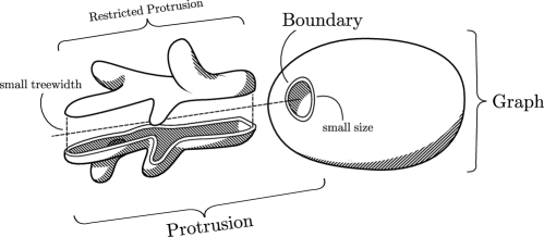
Figure 1: Basic anatomy of a protrusion.

A $t$-boundaried graph is a graph $G=(V,E)$ with a set $\mathop{\mathbf{missing}}{bd}(G)$ (called the boundary or the terminals of $G$) of $t$ distinguished vertices labeled $1$ through $t$. Let $\mathcal{G}_{t}$ denote the class of $t$-boundaried graphs, with graphs from $\mathcal{G}$. If $W\subseteq V$ is an $r$-protrusion in $G$, then we let $G_{W}$ be the $r$-boundaried graph $G[W]$ with boundary $\partial_{G}(W)$, where the vertices of $\partial_{G}(W)$ are assigned labels $1$ through $r$ according to their order in $G$.

Definition 5 (Gluing and ungluing).

For $t$-boundaried graphs $G_{1}$ and $G_{2}$, we let $G_{1}\oplus G_{2}$ denote the graph obtained by taking the disjoint union of $G_{1}$ and $G_{2}$ and identifying each vertex in $\mathop{\mathbf{missing}}{bd}(G_{1})$ with the vertex in $\mathop{\mathbf{missing}}{bd}(G_{2})$ with the same label. This operation is called gluing.

Let $G_{1}$ be a subgraph of a graph $G$ and suppose that $G_{1}$ has a boundary $\mathop{\mathbf{missing}}{bd}(G_{1})$ of size $t$. The operation of ungluing $G_{1}$ from $G$ creates a $t$-boundaried graph, denoted by $G\ominus G_{1}$, and defined as follows:

$$G\ominus G_{1} = G-(V(G_{1})\setminus\mathop{\mathbf{missing}}{bd}(G_{1})),$$

$$\mathop{\mathbf{missing}}{bd}(G\ominus G_{1}) = \mathop{\mathbf{missing}}{bd}(G_{1}).$$

The vertices of $\mathop{\mathbf{missing}}{bd}(G\ominus G_{1})$ are assigned labels $1$ through $t$ according to their order in the graph $G$.

Definition 6 (Replacement).

Let $G=(V,E)$ be a graph with a $t$-protrusion $W$; let $G_{W}$ denote the graph $G[W]$ with boundary $\mathop{\mathbf{missing}}{bd}(G_{W})=\partial_{G}(W)$; and finally, let $G_{1}$ be a $t$-boundaried graph. Then replacing $G_{W}$ by $G_{1}$ corresponds to the operation $(G\ominus G_{W})\oplus G_{1}$.

Definition 7 (Protrusion decomposition).

An $(\alpha,t)$-protrusion decomposition of a graph $G$ is a partition ${\cal P}=Y_{0}\uplus Y_{1}\uplus\cdots\uplus Y_{\ell}$ of $V(G)$ such that:

1. for every $1\leqslant i\leqslant\ell$, $N(Y_{i})\subseteq Y_{0}$;

2. $\max\{\ell,|Y_{0}|\}\leqslant\alpha$;

3. for every $1\leqslant i\leqslant\ell$, $Y_{i}\cup N_{Y_{0}}(Y_{i})$ is a $t$-protrusion of $G$.

The set $Y_{0}$ is called the separating part of $\mathcal{P}$.

Hereafter, the value of $t$ will be fixed to some constant. When $G$ is the input of a parameterized graph problem with parameter $k$, we say that an $(\alpha,t)$-protrusion decomposition of $G$ is linear (resp. quadratic) whenever $\alpha=O(k)$ (resp. $\alpha=O(k^{2})$).

We now restate the definition of one of the most important notions used in this paper.

Definition 8 (Finite integer index (FII) [11]).

Let $\Pi_{\mathcal{G}}$ be a parameterized graph problem restricted to a class $\mathcal{G}$ and let $G_{1},G_{2}$ be two $t$-boundaried graphs in $\mathcal{G}_{t}$. We say that $G_{1}\equiv_{\Pi,t}G_{2}$ if there exists a constant $\Delta_{\Pi,t}(G_{1},G_{2})$ (that depends on $\Pi$, $t$, and the ordered pair $(G_{1},G_{2})$) such that for all $t$-boundaried graphs $G_{3}$ and for all $k$:

1. $G_{1}\oplus G_{3}\in\mathcal{G}$ iff $G_{2}\oplus G_{3}\in\mathcal{G}$;

2. $(G_{1}\oplus G_{3},k)\in\Pi$ iff $(G_{2}\oplus G_{3},k+\Delta_{\Pi,t}(G_{1},G_{2}))\in\Pi$.

We say that the problem $\Pi_{\mathcal{G}}$ has finite integer index in the class $\mathcal{G}$missing iff for every integer $t$, the equivalence relation $\equiv_{\Pi,t}$ has finite index. In the case that $(G_{1}\oplus G,k)\not\in\Pi$ or $G_{1}\oplus G\not\in\mathcal{G}$ for all $G\in\mathcal{G}_{t}$, we set $\Delta_{\Pi,t}(G_{1},G_{2})=0$. Note that $\Delta_{\Pi,t}(G_{1},G_{2})=-\Delta_{\Pi,t}(G_{2},G_{1})$.

If a parameterized problem has finite integer index then its instances can be reduced by “replacing protrusions”. The technique of replacing protrusions hinges on the fact that each protrusion of “large” size can be replaced by a “small” gadget from the same equivalence class as the protrusion, which consequently behaves similarly w.r.t. the problem at hand. If $G_{1}$ is replaced by a gadget $G_{2}$, then the parameter $k$ in the problem changes by $\Delta_{\Pi,t}(G_{1},G_{2})$. What is not immediately clear is that given that a problem $\Pi$ has finite integer index, how does one show that there always exists a set of representatives for which the parameter is guaranteed not to increase. The next lemma shows that this is indeed the case.

Lemma 1.

Let $\Pi$ be a parameterized graph problem that has finite integer index in a graph class $\mathcal{G}$. Then for every fixed $t$, there exists a finite set $\mathcal{R}_{t}$ of $t$-boundaried graphs such that for each $t$-boundaried graph $G\in\mathcal{G}_{t}$ there exists a $t$-boundaried graph $G^{\prime}\in\mathcal{R}_{t}$ such that $G\equiv_{\Pi,t}G^{\prime}$ and $\Delta_{\Pi,t}(G,G^{\prime})\geqslant 0$.

Proof.

The set $\mathcal{R}_{t}$ consists of one element from each equivalence class of $\equiv_{\Pi,t}$. Since $\Pi$ has finite integer index, the set $\mathcal{R}_{t}$ is finite. Therefore we only have to show that there exist representatives that satisfy the requirement in the statement of the lemma.

To this end, fix any equivalence class $\mathcal{G}_{t}^{\prime}\in\mathcal{G}_{t}/\!\!\equiv_{\Pi,t}$. First consider the case where there exists $G_{1}\in\mathcal{G}_{t}^{\prime}$ such that for all $G\in\mathcal{G}_{t}$, either $G_{1}\oplus G\not\in\mathcal{G}$ or for all $k\in\mathbb{N}_{0}$, $(G_{1}\oplus G,k)\not\in\Pi$. Since $\mathcal{G}_{t}^{\prime}$ is an equivalence class, this means that at least one of these two conditions holds for every graph $G\in\mathcal{G}_{t}^{\prime}$. Thus $\Delta_{\Pi,t}(G_{1},G_{2})=0$ for all $t$-boundaried graphs $G_{1},G_{2}\in\mathcal{G}_{t}^{\prime}$ and we can simply take a graph of smallest size from $\mathcal{G}_{t}^{\prime}$ as representative.

We can now assume that for the chosen $\mathcal{G}_{t}^{\prime}$ it holds that there exists a $t$-boundaried graph $G\in\mathcal{G}_{t}$ such that for all $G_{1}\in\mathcal{G}_{t}^{\prime}$ we have that $G_{1}\oplus G\in\mathcal{G}$ and, for some $k\in\mathbb{N}$, $(G_{1}\oplus G,k)\in\Pi_{\mathcal{G}}$. Consider the following binary relation $\preceq$ over $\mathcal{G}_{t}^{\prime}$: for all $G_{1},G_{2}\in\mathcal{G}_{t}^{\prime}$,

$$G_{1}\preceq G_{2}\Leftrightarrow\Delta_{\Pi,t}(G_{1},G_{2})\geqslant 0.$$

As $\Delta_{\Pi,t}(G,G)=0$ for all $G\in\mathcal{G}_{t}$, it immediately follows that the relation $\preceq$ is reflexive. Furthermore, the relation is total as every graph is comparable to every other graph from the same equivalence class.

We next show that the relation $\preceq$ is also transitive, making it a total quasi-order. Let $G_{1},G_{2},G_{3}\in\mathcal{G}_{t}^{\prime}$ be such that $G_{1}\preceq G_{2}$ and $G_{2}\preceq G_{3}$. This is equivalent to saying that $c_{12}=\Delta_{\Pi,t}(G_{1},G_{2})\geqslant 0$ and $c_{23}=\Delta_{\Pi,t}(G_{2},G_{3})\geqslant 0$. For every $G\in\mathcal{G}_{t}$ such that $G_{1}\oplus G\in\mathcal{G}$ and $(G_{1}\oplus G,k)\in\Pi$ for some $k\in\mathbb{N}$, we have

$$(G_{1}\oplus G,k)\in\Pi \Leftrightarrow (G_{2}\oplus G,k+c_{12})\in\Pi$$

$$\Leftrightarrow (G_{3}\oplus G,k+c_{12}+c_{23})\in\Pi.$$

By definition, $\Delta_{\Pi,t}(G_{1},G_{3})=c_{12}+c_{23}\geqslant 0$ and hence $G_{1}\preceq G_{3}$. We conclude that $\preceq$ is transitive and therefore a total quasi-order.

We now show that the class $\mathcal{G}_{t}^{\prime}$ can be partitioned into layers that can be linearly ordered. We will pick our representative for the class $\mathcal{G}_{t}^{\prime}$ from the first layer in this ordering. To do this, we define the following equivalence relation over $\mathcal{G}_{t}^{\prime}$. For all $G_{1},G_{2}\in\mathcal{G}_{t}^{\prime}$, define

$$G_{1}\equiv G_{2} \Leftrightarrow G_{1}\preceq G_{2}~{}\textnormal{and}~{}G_{2}\preceq G_{1}$$

$$\Leftrightarrow \Delta_{\Pi,t}(G_{1},G_{2})=0.$$

Now, the equivalence classes $\mathcal{G}_{t}^{\prime}/\!\!\equiv$ can be linearly ordered as follows. Fix a graph $G\in\mathcal{G}_{t}$ such that for any $G_{1}\in\mathcal{G}_{t}^{\prime}$ we have that $G_{1}\oplus G\in\mathcal{G}$ and $(G_{1}\oplus G,k)\in\Pi$ for some $k\in\mathbb{N}$, this graph must exist since we handled equivalence classes of $\mathcal{G}_{t}/\!\!\equiv_{\Pi,t}$ which do not have such a graph in the first part of the proof. Consider the function $\Phi_{G}\colon\mathcal{G}_{t}^{\prime}/\!\!\equiv\rightarrow\mathbb{N}_{0}$ defined via

$$\Phi_{G}([G^{\prime}])=\min\left\{k\in\mathbb{N}\mid(G^{\prime}\oplus G,k)\in\Pi\right\}.$$

Observe that $\Phi_{G}([G_{2}])=\Phi_{G}([G_{1}])+\Delta_{\Pi,t}(G_{1},G_{2})$ for all $G_{1},G_{2}\in\mathcal{G}_{t}^{\prime}$ and, in particular, that

$$\Phi_{G}([G_{1}])=\Phi_{G}([G_{2}])\Leftrightarrow G_{1}\equiv G_{2}.$$

Thus $\Phi_{G}$ induces a linear order on $\mathcal{G}_{t}^{\prime}/\!\!\equiv$. Moreover, since $\Phi_{G}(\cdot)\geqslant 0$, there exists a class $[G^{*}]$ in $\mathcal{G}_{t}^{\prime}/\!\!\equiv$ that is a minimum element in the order induced by $\Phi_{G}$. For any $t$-boundaried graph $G\in[G^{*}]$, it then follows that for all $G_{1}\in\mathcal{G}_{t}^{\prime}$, $\Delta_{\Pi,t}(G,G_{1})\geqslant 0$. The representative of $\mathcal{G}_{t}^{\prime}$ in $\mathcal{R}_{t}$ is an arbitrary $t$-boundaried graph $G^{\prime}\in[G^{*}]$ of smallest size. This proves the lemma. ∎

We now show that the protrusion reduction rule is safe.

Lemma 2 (Safety).

Let $\mathcal{G}$ be a graph class and let $\Pi_{\mathcal{G}}$ be a parameterized graph problem with finite integer index w.r.t. $\mathcal{G}$. If $(G^{\prime},k^{\prime})$ is the instance obtained from one application of the protrusion reduction rule to the instance $(G,k)$ of $\Pi_{\mathcal{G}}$, then

1. $G^{\prime}\in\mathcal{G}$;

2. $(G^{\prime},k^{\prime})$ is a Yes-instance iff $(G,k)$ is a Yes-instance; and

3. $k^{\prime}\leqslant k$.

Proof.

Suppose that $(G^{\prime},k^{\prime})$ is obtained from $(G,k)$ by replacing a $2t$-boundaried subgraph $G_{W}$ (induced by a $2t$-protrusion $W$) by a representative $G_{1}\in\mathcal{R}_{2t}$. Let $\tilde{G}$ be the $2t$-boundaried graph $G-W^{\prime}$, where $W^{\prime}$ is the restricted protrusion of $W$ and $B(\tilde{G})=\partial_{G}(W)$. Since $G_{W}\equiv_{\Pi,2t}G_{1}$, we have by Definition 8,

1. $G=\tilde{G}\oplus G_{W}\in\mathcal{G}$ iff $\tilde{G}\oplus G_{1}\in\mathcal{G}$.

2. $(\tilde{G}\oplus G_{W},k)\in\Pi_{\mathcal{G}}$ iff $(\tilde{G}\oplus G_{1},k-\Delta_{\Pi,2t}(G_{1},G_{W}))\in\Pi_{\mathcal{G}}$.

Hence $G^{\prime}=\tilde{G}\oplus G_{1}\in\mathcal{G}$. Lemma 1 ensures that $\Delta_{\Pi,2t}(G_{1},G_{W})\geqslant 0$, and hence $k^{\prime}=k-\Delta_{\Pi,2t}(G_{1},G_{W}))\leqslant k$. ∎

In what follows, unless otherwise stated, when applying protrusion replacement rules we will assume that for each $t\in\mathbb{N}$, we are given the set $\mathcal{R}_{t}$ of representatives of the equivalence classes of $\equiv_{\Pi_{\mathcal{G}},t}$. The representatives are chosen in accordance with the condition stated in Lemma 1 so that for all $G\in\mathcal{R}_{t}$ and all $G^{\prime}\equiv_{\Pi_{\mathcal{G}},t}G$, we have that $\Delta_{\Pi_{\mathcal{G}},t}(G,G^{\prime})\geqslant 0$. Note that this makes our algorithms of Section 4 non-uniform. However non-uniformity is implicitly assumed in previous work that used the protrusion machinery for designing kernelization algorithms [7, 37, 33, 35].

Definition 9 (Protrusion limit).

For a parameterized graph problem $\Pi$ that has finite integer index in the class $\mathcal{G}$, let $\mathcal{R}_{t}$ denote the set of representatives of the equivalence classes of $\equiv_{\Pi,t}$ as in Lemma 1. The protrusion limit of $\Pi_{\mathcal{G}}$ is a function $\rho_{\Pi_{\mathcal{G}}}\colon\mathbb{N}\rightarrow\mathbb{N}$ defined as $\rho_{\Pi_{\mathcal{G}}}(t)=\max_{G\in\mathcal{R}_{t}}|V(G)|$. We drop the subscript when it is clear which graph problem is being referred to. We also define $\rho^{\prime}(t):=\rho(2t)$.

The next two lemmas deal with finding protrusions in graphs. The first of these guarantees that whenever there exists a “large enough” protrusion there exists a protrusion that is large but bounded by a constant (that depends on the problem and the boundary size). As we shall see later, the fact that we deal with protrusions of constant size enables us to efficiently test which representative to replace them by, assuming that we have the set of representatives. For completeness, we provide the proof of the following lemma.

Lemma 3 (​[7]).

Let $\Pi$ be a parameterized graph problem with finite integer index in $\mathcal{G}$ and let $t\in\mathbb{N}$ be a constant. For a graph $G\in\mathcal{G}$, if one is given a $t$-protrusion $X\subseteq V(G)$ such that $\rho^{\prime}_{\Pi_{\mathcal{G}}}(t)<|X|$, then one can, in time $O(|X|)$, find a $2t$-protrusion $W$ such that $\rho^{\prime}_{\Pi_{\mathcal{G}}}(t)<|W|\leqslant 2\cdot\rho^{\prime}_{\Pi_{\mathcal{G}}}(t)$.

Proof.

Let $(T,\mathcal{X})$ be a nice tree-decomposition for $G[X]$ of width $t-1$. Root $T$ at an arbitrary node. Let $u$ be the lowest node of $T$ such that if $W$ is the set of vertices in the bags associated with the nodes in the subtree $T_{u}$ rooted at $u$, then $|W|>\rho^{\prime}_{\Pi_{\mathcal{G}}}(t)$. Clearly $W$ is a $2t$-protrusion with boundary $X_{u}\cup\partial_{G}(X)$, where $X_{u}\subseteq V(G)$ is the bag associated with the node $u$ of $T$. By the choice of $u$, it is clear that $u$ cannot be a forget node. If $u$ is an introduce node with child $v$, then the number of vertices in the bags associated with the nodes of $T_{v}$ must be exactly $\rho^{\prime}_{\Pi_{\mathcal{G}}}(t)$. Since $u$ introduces an additional vertex of $G$, we have $|W|=\rho^{\prime}_{\Pi_{\mathcal{G}}}(t)+1$. Finally consider the case when $u$ is a join node with children $y,z$. Then the bags associated with these nodes $X_{u},X_{y},X_{z}$ are identical and since

$$\big{|}\,\bigcup_{\mathclap{j\in V(T_{y})}}X_{j}\,\big{|}<\rho^{\prime}_{\Pi_{\mathcal{G}}}(t)\qquad\text{and}\qquad\big{|}\,\bigcup_{\mathclap{j\in V(T_{z})}}X_{j}\,\big{|}<\rho^{\prime}_{\Pi_{\mathcal{G}}}(t),$$

we have that $W=\bigcup_{j\in V(T_{y})}X_{j}\cup\bigcup_{j\in V(T_{z})}X_{j}$ has size at most $2\cdot\rho^{\prime}_{\Pi_{\mathcal{G}}}(t)$.

Computing a nice tree-decomposition $(T,\mathcal{X})$ of $G[X]$ takes time $O(2^{O(t^{3})}\cdot|X|)$ [6] and the time required to compute a $2t$-protrusion from $T$ is $O(|X|)$. Since $t$ is a constant, the total time taken is $O(|X|)$. ∎

For a fixed $t$, the protrusion $W$ is of constant size but, in the reduction rule to be described, would be replaced by a representative of size at most $\rho_{\Pi_{\mathcal{G}}}(2t)$. This means that each time the reduction rule is applied, the size of the graph strictly decreases and, by Lemma 1, the parameter does not increase. The reduction rule can therefore be applied at most $n$ times, where $n$ is the number of vertices in the input graph. As we shall see later, each application of the reduction rule takes time polynomial in $n$, assuming that we are given the set of representatives. Therefore, in polynomial time, we would obtain an instance in which every $t$-protrusion has size at most $\rho_{\Pi_{\mathcal{G}}}(2t)$. This trick is described in [7] but is stated here for the sake of completeness.

The next lemma describes how to find a $t$-protrusion of maximum size.

Lemma 4 (Finding maximum sized protrusions).

Let $t$ be a constant. Given an $n$-vertex graph $G$, a $t$-protrusion of $G$ with the maximum number of vertices can be found in time $O(n^{t+1})$.

Proof.

For a vertex set $B\subseteq V(G)$ of size at most $t$, let $C_{B,1},\ldots,C_{B,p}$ be the connected components of $G-B$ such that, for $1\leqslant i\leqslant p$, $\mathop{\mathbf{missing}}{tw}(G[V(C_{B,i})\cup B])\leqslant t$. The connected components of $G-B$ can be determined in $O(n)$ time and one can test whether the graph induced by $V(C_{B,i})\cup B$ has treewidth at most $t-1$ in time $O(2^{O(t^{3})}\cdot n)$ [6]. Since we have assumed that $t$ is a fixed constant, deciding whether the treewidth is within $t-1$ can be done in linear time. By definition, $\bigcup_{i=1}^{p}V(C_{B,i})\cup B$ is a $t$-protrusion with boundary $B$. Conversely every $t$-protrusion $W$ consists of a boundary $\partial(W)$ of size at most $t$ such that the restricted protrusion $W^{\prime}=W\setminus\partial(W)$ is a collection of connected components $C$ of $G-\partial(W)$ satisfying the condition $\mathop{\mathbf{missing}}{tw}(G[V(C)\cup\partial(W)])\leqslant t-1$. Therefore to find a $t$-protrusion of maximum size, one simply runs through all vertex sets $B$ of size at most $t$ and for each set determines the maximum $t$-protrusion with boundary $B$. The largest $t$-protrusion over all choices of the boundary $B$ is a largest $t$-protrusion in the graph. All of this takes time $O(n^{t+1})$. ∎

Finally, given a $2t$-protrusion $W$ with the desired size constraints, we show how to determine which representative of our equivalence class is equivalent to $G[W]$.

Lemma 5.

Let $\Pi$ be a parameterized graph problem that has finite integer index on $\mathcal{G}$. For $t\in\mathbb{N}$, a constant, suppose that the set $\mathcal{R}_{t}$ of representatives of the equivalence relation $\equiv_{\Pi,t}$ is given. If $W$ is a $t$-protrusion of size at most $c$, a fixed constant, then one can decide in constant time which $G^{\prime}\in\mathcal{R}_{t}$ satisfies $G^{\prime}\equiv_{\Pi,t}G[W]$.

Proof.

Fix $G^{\prime}\in\mathcal{R}_{t}$. We wish to test whether $G^{\prime}\equiv_{\Pi,t}G[W]$. For each $\tilde{G}\in\mathcal{R}_{t}$, solve the problem $\Pi$ on the constant-sized instances $G[W]\oplus\tilde{G}$ and $G^{\prime}\oplus\tilde{G}$ and let $s(G[W],\tilde{G})$ and $s(G^{\prime},\tilde{G})$ denote the size of the optimal solution. Then by the definition of finite integer index, we have $G^{\prime}\equiv_{\Pi,t}G[W]$ if and only if $s(G[W],\tilde{G})-s(G^{\prime},\tilde{G})$ is the same for all $\tilde{G}\in\mathcal{R}_{t}$. To find out which graph in $\mathcal{R}_{t}$ is the correct representative of $G[W]$, we run this test for each graph in $\mathcal{R}_{t}$, of which there are a constant number. The total time taken is, therefore, a constant. ∎

3 Constructing protrusion decompositions

In this section we present our algorithm to compute protrusion decompositions. Our approach is based on an algorithm which marks the bags of a tree-decomposition of an input graph $G$ that comes equipped with a subset $X\subseteq V(G)$ such that the graph $G-X$ has bounded treewidth. Let henceforth $t$ be an integer such that $\mathop{\mathbf{missing}}{tw}(G-X)\leqslant t-1$ and let $r$ be an integer that is also given to the algorithm. This parameter $r$ will depend on the particular graph class to which $G$ belongs and the precise problem one might want to solve (see Sections 4 and 5 for more details). More precisely, given optimal tree-decompositions of the connected components of $G-X$ with at least $r$ neighbors in $X$, the bag marking algorithm greedily identifies a set of bags $\mathcal{M}$ in a bottom-up manner. The set $V(\mathcal{M})$ of vertices contained in marked bags together with $X$ will form the separating part $Y_{0}$ of the protrusion decomposition. Intuitively, the marked bags will be mapped bijectively into a collection of pairwise vertex-disjoint connected subgraphs of $G-X$, each of which has a large neighborhood in $X$ (namely, of size greater than $r$), implying in several particular cases a limited number of marked bags (see Sections 4 and 5). In order to guarantee that the connected components of $G-(X\cup V(\mathcal{M}))$ form protrusions with small boundary, the set $\mathcal{M}$ is closed under taking LCA’s (least common ancestors; see Lemma 7). The precise description of the procedure can be found in Algorithm 1 below and a sketch of the decomposition is depicted in Figure 2.

Input: A graph $G$, a subset $X\subseteq V(G)$ such that $\mathop{\mathbf{missing}}{tw}(G-X)\leqslant t-1$, and an integer $r>0$.

Set $\mathcal{M}\leftarrow\emptyset$ as the set of marked bags;

Compute an optimal rooted tree-decomposition $\mathcal{T}_{C}=(T_{C},\mathcal{B}_{C})$ of every connected component $C$ of $G-X$ such that $|N_{X}(C)|\geqslant r$;

Repeat the following loop for every rooted tree-decomposition $\mathcal{T}_{C}$;

while $\mathcal{T}_{C}$ contains an unprocessed bag do

      

      Let $B$ be an unprocessed bag at the farthest distance from the root of $\mathcal{T}_{C}$;

       [LCA marking step]

       if $B$ is the LCA of two marked bags of $\mathcal{M}$missing then

             $\mathcal{M}\leftarrow\mathcal{M}\cup\{B\}$ and remove the vertices of $B$ from every bag of $\mathcal{T}_{C}$;

            

      

      [Large-subgraph marking step]

       else if $G_{B}$ contains a connected component $C_{B}$ such that $|N_{X}(C_{B})|\geqslant r$missing then

             $\mathcal{M}\leftarrow\mathcal{M}\cup\{B\}$ and remove the vertices of $B$ from every bag of $\mathcal{T}_{C}$;

            

      

      Bag $B$ is now processed;

      

return $Y_{0}=X\cup V(\mathcal{M})$missing;

Algorithm 1 Bag marking algorithm

Before we discuss properties of the set $\mathcal{M}$ of marked bags and the set $Y_{0}=X\cup V(\mathcal{M})$, let us establish the time complexity of the bag marking algorithm and describe how the dynamic programming is done in the Large-subgraph marking step. Since the dynamic programming procedure is quite standard, we just sketch the main ideas.

Implementation and time complexity of Algorithm 1.

First, an optimal tree-decomposition of every connected component $C$ of $G-X$ such that $|N_{X}(C)|\geqslant r$ can be computed in time linear in $n=|V(G)|$ using the algorithm of Bodlaender for graphs of bounded treewidth [6]. We root such tree-decomposition at an arbitrary bag. For the sake of simplicity of the analysis, we can assume that the tree-decompositions are nice, but it is not necessary for the algorithm.

Note that the LCA marking step can clearly be performed in linear time. Let us now briefly discuss how we can detect, in the Large-subgraph marking step, if a graph $G_{B}$ contains a connected component $C_{B}$ such that $|N_{X}(C_{B})|\geqslant r$ using dynamic programming. For each bag $B$ of the tree-decomposition, we have to keep track of which vertices of $B$ belong to the same connected component of $G_{B}$.

Note that we only need to remember the connected components of the graph $G_{B}$ which intersect $B$, as the other ones will never be connected to the rest of the graph. For each such connected component $C_{B}$ intersecting $B$, we also store $N_{X}(C_{B})$, and note that by definition of the algorithm, it follows that for non-marked bags $B$, $|N_{X}(C_{B})|<r$. At a “join” bag $J$ with children $B_{1}$ and $B_{2}$, we merge the connected components of $G_{B_{1}}$ and $G_{B_{2}}$ sharing at least one vertex (which is necessarily in $J$), and update their neighborhood in $X$ accordingly. If for some of these newly created connected components $C_{J}$ of $G_{J}$, it holds that $|N_{X}(C_{J})|\geqslant r$, then the bag $J$ needs to be marked. At a “forget” bag $F$ corresponding to a forgotten vertex $v$, we only have to forget the connected component $C$ of $G_{F}$ containing $v$ if $V(C)\cap F=\emptyset$. Finally, at an “introduce” bag $I$ corresponding to a new vertex $v$, we have to merge the connected components of $G_{I}$ after the addition of vertex $v$, and update the neighbors in $X$ according to the neighbors of $v$ in $X$.

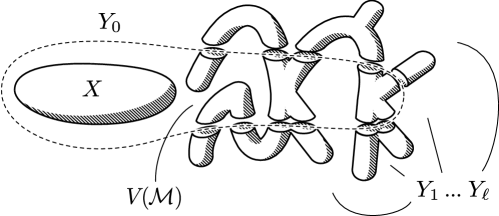
Figure 2: A sketch of how the marking algorithm obtains a protrusion decomposition. $X$ denotes a treewidth-modulator. Edges among the individual vertex sets are not depicted.

Note that for each bag $B$, the time needed to update the information about the connected components of $G_{B}$ depends polynomially on $t$ and $r$. In order for the whole algorithm to run in linear time, we can deal with the removal of marked vertices in the following way. Instead of removing them from every bag of the tree-decomposition, we can just label them as “marked” when marking a bag $B$, and just not take them into account when processing further bags.

The next lemma follows from the above discussion.

Lemma 6.

Algorithm 1 can be implemented to run in $O(n)$ time, where the hidden constant depends only on $t$ and $r$.

Basic properties of Algorithm 1.

Denote by $\mathcal{T}$ the union of the set of optimal tree-decompositions $\mathcal{T}_{C}$ of every connected component $C$ of $G-X$ with at least $r$ neighbors in $X$.

Lemma 7.

If $T$ is a maximal connected subtree of $\mathcal{T}$ not containing any marked bag of $\mathcal{M}$, then $T$ is adjacent to at most two marked bags of $\mathcal{T}$.

Proof.

As that every tree-decomposition in $\mathcal{T}$ is rooted, so is any maximal subtree $T$ of $\mathcal{T}$ not containing any marked bag of $\mathcal{M}$. Assume that $\mathcal{M}$ contains two distinct marked bags, say $B_{1}$ and $B_{2}$, each adjacent to a leaf of $T$. As $T$ is connected, observe that the LCA $B$ of $B_{1}$ and $B_{2}$ belongs to $T$. Since $\mathcal{M}$ is closed under taking LCA, $T$ contains a marked bag $B$, a contradiction. It follows that $T$ is adjacent to at most two marked bags: a unique one adjacent to a leaf, and possibly another one adjacent to its root. ∎

As a consequence of the previous lemma we can now argue that every connected component of $G-Y_{0}$ has a small neighborhood in $X$ and thus forms a restricted protrusion.

Lemma 8.

Let $Y_{0}$ be the set of vertices computed by Algorithm 1. Every connected component $C$ of $G-Y_{0}$ satisfies $|N_{X}(C)|<r$ and $|N_{Y_{0}}(C)|<r+2t$.

Proof.

Let $C$ be a connected component of $G-Y_{0}$. Observe that $C$ is contained in a connected component $C_{X}$ of $G-X$ such that either $|N_{X}(C_{X})|<r$ or $|N_{X}(C_{X})|\geqslant r$. In the former case, as Algorithm 1 does not mark any vertex of $C_{X}$, $C=C_{X}$ and so $|N_{Y_{0}}(C)|<r+2t$ trivially holds. So assume that $|N_{X}(C_{X})|\geqslant r$. Then $C_{X}$ has been chopped by Algorithm 1 and clearly $C\subseteq C_{X}\setminus V(\mathcal{M})$. More precisely, if $\mathcal{T}_{C_{X}}$ is the rooted tree-decomposition of $C_{X}$, there exists a maximal connected subtree $T$ of $\mathcal{T}_{C_{X}}$ not containing any marked bag such that $C\subseteq V(T)\setminus V(\mathcal{M})$. By construction of $\mathcal{M}$, every connected component of the subgraph induced by $V(T)\setminus V(\mathcal{M})$ has strictly less than $r$ neighbors in $X$ (otherwise the root of $T$ or one of its descendants would have been marked at the Large-subgraph marking step). It follows that $|N_{X}(C)|<r$. To conclude, observe that Lemma 7 implies that the neighbors of $C$ in $V(\mathcal{M})$ are contained in at most two marked bags of $\mathcal{T}$. It follows that $|N_{Y_{0}}(C)|<r+2t$. ∎

Given a graph $G$ and a subset $S\subseteq V(G)$, we define a cluster of $G-S$missing as a maximal collection of connected components of $G-S$ with the same neighborhood in $S$. Note that the set of all clusters of $G-S$ induces a partition of the set of connected components of $G-S$, which can be easily found in linear time if $G$ and $S$ are given.

By Lemma 8 and using the fact that $\mathop{\mathbf{missing}}{tw}(G-X)\leqslant t-1$, the following proposition follows.

Proposition 1.

Let $r,t$ be two positive integers, let $G$ be a graph and $X\subseteq V(G)$ such that $\mathop{\mathbf{missing}}{tw}(G-X)\leqslant t-1$, let $Y_{0}\subseteq V(G)$ be the output of Algorithm 1 with input $(G,X,r)$, and let $Y_{1},\ldots,Y_{\ell}$ be the set of all clusters of $G-Y_{0}$. Then $\mathcal{P}:=Y_{0}\uplus Y_{1}\uplus\cdots\uplus Y_{\ell}$ is a $(\max\{\ell,|Y_{0}|\},2t+r)$-protrusion decomposition of $G$.

In other words, each cluster of $G-Y_{0}$ is a restricted $(2t+r)$-protrusion. Note that Proposition 1 neither bounds $\ell$ or $|Y_{0}|$. In the sequel, we will use Algorithm 1 and Proposition 1 to give explicit bounds on $\ell$ and $|Y_{0}|$, in order to achieve two different results. In Section 4 we use Algorithm 1 and Proposition 1 to obtain linear kernels for a large class of problems on sparse graphs. In Section 5 we use Algorithm 1 and Proposition 1 to obtain a single-exponential algorithm for the parameterized Planar-$\mathcal{F}$-Deletion problem.

4 Linear kernels on graphs excluding a topological minor

In this section we prove Theorem I. We then state a number of concrete problems that satisfy the structural constraints imposed by this theorem (Subsection 4.1), discuss these constraints in the context of previous work in this area (Subsection 4.2), and trace graph classes to which our approach can be lifted (Subsection 4.3). Finally, in Subsection 4.4 we discuss how to use the machinery developed in proving Theorem I to obtain a concrete kernel for the Edge Dominating Set problem.

With the protrusion machinery outlined in Section 2 at hand, we can now describe the protrusion reduction rule. Informally, we find a sufficiently large $t$-protrusion (for some yet to be fixed constant $t$), replace it with a small representative, and change the parameter accordingly. In the following, we will drop the subscript from the protrusion limit functions $\rho_{\Pi}$ and $\rho^{\prime}_{\Pi}$.

Reduction Rule 1 (Protrusion reduction rule).

Let $\Pi_{\mathcal{G}}$ denote a parameterized graph problem restricted to some graph class $\mathcal{G}$, let $(G,k)\in\Pi_{\mathcal{G}}$ be a Yes-instance of $\Pi_{\mathcal{G}}$, and let $t\in\mathbb{N}$ be a constant. Suppose that $W^{\prime}\subseteq V(G)$ is a $t$-protrusion of $G$ such that $|W^{\prime}|>\rho^{\prime}(t)$. Let $W\subseteq V(G)$ be a $2t$-protrusion of $G$ such that $\rho^{\prime}(t)<|W|\leqslant 2\cdot\rho^{\prime}(t)$, obtained as described in Lemma 3. We let $G_{W}$ denote the $2t$-boundaried graph $G[W]$ with boundary $\mathop{\mathbf{missing}}{bd}(G_{W})=\partial_{G}(W)$. Let further $G_{1}\in\mathcal{R}_{2t}$ be the representative of $G_{W}$ for the equivalence relation $\equiv_{\Pi,|\partial(W)|}$ as defined in Lemma 1.

The protrusion reduction rule (for boundary size $t$) is the following:

Reduce $(G,k)$ to $(G^{\prime},k^{\prime})=(G[V\setminus W^{\prime}]\oplus G_{1},k-\Delta_{\Pi,2t}(G_{1},G_{W}))$missing.

By Lemma 1, the parameter in the new instance does not increase. We now show that the protrusion reduction rule is safe.

Lemma 9 (Safety).

Let $\mathcal{G}$ be a graph class and let $\Pi_{\mathcal{G}}$ be a parameterized graph problem with finite integer index w.r.t. $\mathcal{G}$. If $(G^{\prime},k^{\prime})$ is the instance obtained from one application of the protrusion reduction rule to the instance $(G,k)$ of $\Pi_{\mathcal{G}}$, then

1. $G^{\prime}\in\mathcal{G}$;

2. $(G^{\prime},k^{\prime})$ is a Yes-instance iff $(G,k)$ is a Yes-instance; and

3. $k^{\prime}\leqslant k$.

Proof.

Suppose that $(G^{\prime},k^{\prime})$ is obtained from $(G,k)$ by replacing a $2t$-boundaried subgraph $G_{W}$ (induced by a $2t$-protrusion $W$) by a representative $G_{1}\in\mathcal{R}_{2t}$. Let $\tilde{G}$ be the $2t$-boundaried graph $G-W^{\prime}$, where $W^{\prime}$ is the restricted protrusion of $W$ and $B(\tilde{G})=\partial_{G}(W)$. Since $G_{W}\equiv_{\Pi,2t}G_{1}$, we have by Definition 8,

1. $G=\tilde{G}\oplus G_{W}\in\mathcal{G}$ iff $\tilde{G}\oplus G_{1}\in\mathcal{G}$.

2. $(\tilde{G}\oplus G_{W},k)\in\Pi_{\mathcal{G}}$ iff $(\tilde{G}\oplus G_{1},k-\Delta_{\Pi,2t}(G_{1},G_{W}))\in\Pi_{\mathcal{G}}$.

Hence $G^{\prime}=\tilde{G}\oplus G_{1}\in\mathcal{G}$. Lemma 1 ensures that $\Delta_{\Pi,2t}(G_{1},G_{W})\geqslant 0$, and hence $k^{\prime}=k-\Delta_{\Pi,2t}(G_{1},G_{W}))\leqslant k$. ∎

Observation 1.

If $(G,k)$ is reduced w.r.t. the protrusion reduction rule with boundary size $\beta$, then for all $t\leqslant\beta$, every $t$-protrusion $W$ of $G$ has size at most $\rho^{\prime}(t)$.

In order to obtain linear kernels, we require the problem instances to have more structure. In particular, we adapt the notion of quasi-compactness introduced in [7] to define what we call treewidth-bounding.

Definition 10 (Treewidth-bounding).

A parameterized graph problem $\Pi$ is called $(s,t)$-treewidth-bounding if there exists a function $s\colon\mathbb{N}\rightarrow\mathbb{N}$ and a constant $t$ such that for every $(G,k)\in\Pi$ there exists $X\subseteq V(G)$ such that:

1. $|X|\leqslant s(k)$; and

2. $\mathop{\mathbf{missing}}{tw}(G-X)\leqslant t-1$.

We call a problem treewidth-bounding on a graph class $\mathcal{G}$missing if the above property holds under the restriction that $G\in\mathcal{G}$. We call $X$ a $t$-treewidth-modulator of $G$, $s$ the treewidth-modulator size and $t$ the treewidth bound of the problem $\Pi$.

We assume in the following that the problem $\Pi$ at hand is treewidth-bounding with bound $t$ and modulator size $s(\cdot)$, that is, a Yes-instance $(G,k)\in\Pi_{\mathcal{G}}$ has a modulator set $X\subseteq V(G)$ with $|X|\leqslant s(k)$ and $\mathop{\mathbf{missing}}{tw}(G-X)\leqslant t-1$. Note that in general $s,t$ depend on $\Pi$ and $\mathcal{G}$. For many problems that are treewidth-bounding, such as Vertex Cover, Feedback Vertex Set, Treewidth-$t$ Vertex Deletion, the set $X$ is actually the solution set. However, in general, $X$ could be any vertex set and does not have to be given nor efficiently computable to obtain a kernel. The fact that it exists is all we need for our proof to go through.

The rough idea of the proof of Theorem I is as follows. We assume that the given instance $(G,k)$ is reduced w.r.t. the protrusion reduction rule for some yet to be fixed constant boundary size $\beta$. Consequently, every $\beta$-protrusion of $G$ has size at most $\rho^{\prime}(\beta)$. For a protrusion decomposition $Y_{0}\uplus Y_{1}\uplus\cdots\uplus Y_{\ell}$ obtained from Algorithm 1 with a carefully chosen threshold, we can then show that $|Y_{0}|=O(k)$ using properties of $H$-topological-minor-free graphs. The bound on the total size of the clusters of $G-Y_{0}$ then follows from these properties and from the protrusion reduction rule.
We first prove a result (Theorem 1) that is slightly more general than Theorem I and identifies all the key ingredients needed for our result. To do this, we use a sequence of lemmas (10, 11, 12) which bounds the total size of the clusters of the protrusion decomposition. To this end, we define the constriction operation, which essentially shrinks paths into edges.

Definition 11 (Constriction).

Let $G$ be a graph and let $\mathcal{P}$ be a set of paths in $G$ such that for each $P\in\mathcal{P}$ it holds that:

1. the endpoints of $P$ are not connected by an edge in $G$; and

2. for all $P^{\prime}\in\mathcal{P}$, with $P^{\prime}\neq P$, $P$ and $P^{\prime}$ share at most a single vertex which must also be an endpoint of both

We define the constriction of $G$ under $\mathcal{P}$, written $G|_{\mathcal{P}}$, as the graph $H$ obtained by connecting the endpoints of each $P\in\mathcal{P}$ by an edge and then removing all inner vertices of $P$.

We say that $H$ is a $d$-constriction of $G$ if there exists $G^{\prime}\subseteq G$ and a set of paths $\mathcal{P}$ in $G^{\prime}$ such that $d=\max_{P\in\mathcal{P}}|P|$ and $H=G^{\prime}|_{\mathcal{P}}$. Given graph classes $\mathcal{G},\mathcal{H}$ and some integer $d\geqslant 2$, we say that $\mathcal{G}$ $d$-constricts into $\mathcal{H}$missing if for every $G\in\mathcal{G}$, every possible $d$-constriction $H$ of $G$ is contained in the class $\mathcal{H}$. For the case that $\mathcal{G}=\mathcal{H}$ we say that $\mathcal{G}$ is closed under $d$-constrictions. We will call $\mathcal{H}$ the witness class, as the proof of Theorem 1 works by taking an input graph $G$ and constricting it into some witness graph $H$ whose properties will yield the desired bound on $|G|$. We let $\omega(G)$ denote the size of a largest clique in $G$ and $\#\omega(G)$ the total number of cliques in $G$ (not necessarily maximal ones).

Theorem 1.

Let $\mathcal{G},\mathcal{H}$ be graph classes closed under taking subgraphs such that $\mathcal{G}$ $d$-constricts into $\mathcal{H}$ for a fixed constant $d\in\mathbb{N}$. Assume that $\mathcal{H}$ has the property that there exists functions $f_{E},f_{\#\omega}\colon\mathbb{N}\rightarrow\mathbb{N}$ and a constant $\omega_{\mathcal{H}}$ (depending only on $\mathcal{H}$) such that for each graph $H\in\mathcal{H}$ the following conditions hold:

$$|E(H)|\leqslant f_{E}(|H|),\enskip\#\omega(H)\leqslant f_{\#\omega}(|H|),\enskip\text{and}\enskip\omega(H)<\omega_{\mathcal{H}}.$$

Let $\Pi$ be a parameterized graph problem that has finite integer index and is $(s,t)$-treewidth-bounding, both on the graph class $\mathcal{G}$. Define $x_{k}:=s(k)+2t\cdot f_{E}(s(k))$. Then any reduced instance $(G,k)\in\Pi$ has a protrusion decomposition $V(G)=Y_{0}\uplus Y_{1}\uplus\cdots\uplus Y_{\ell}$ such that:

1. $|Y_{0}|\leqslant x_{k}$;

2. $|Y_{i}|\leqslant\rho^{\prime}(2t+\omega_{\mathcal{H}})$ for $1\leqslant i\leqslant\ell$; and

3. $\ell\leqslant f_{\#\omega}(x_{k})+x_{k}+1$.

Hence $\Pi$ restricted to $\mathcal{G}$ admits kernels of size at most

$$x_{k}+(f_{\#\omega}(x_{k})+x_{k}+1)\rho^{\prime}(2t+\omega_{\mathcal{H}}).$$

We split the proof of Theorem 1 into several lemmas. First, let us fix the way in which the decomposition $Y_{0}\uplus Y_{1}\uplus\cdots\uplus Y_{\ell}$ is obtained: given a reduced Yes-instance $(G,k)\in\mathcal{G}$, let $X\subseteq V(G)$ be a treewidth-modulator of size at most $|X|\leqslant s(k)$ such that $\mathop{\mathbf{missing}}{tw}(G-X)\leqslant t-1$. We run Algorithm 1 on the input $(G,X,\omega_{\mathcal{H}})$.

Lemma 10.

The protrusion decomposition $Y_{0}\uplus Y_{1}\uplus\cdots\uplus Y_{\ell}$ obtained by running Algorithm 1 on $(G,X,\omega_{\mathcal{H}})$ has the following properties:

1. For each $1\leqslant i\leqslant\ell$, we have $|Y_{i}|\leqslant\rho^{\prime}(2t+\omega_{\mathcal{H}})$;

2. For each connected subgraph $C_{B}$ witnessed by Algorithm 1 in the “Large-subgraph marking step”, $|C_{B}|\leqslant\rho^{\prime}(2t+\omega_{\mathcal{H}})+t$.

Proof.

The first claim follows directly from Lemma 8: for each $1\leqslant i\leqslant\ell$, we have $|N_{Y_{0}}(Y_{i})|\leqslant 2t+\omega_{\mathcal{H}}$. As $Y_{i}\subseteq G-X$, it follows that $\mathop{\mathbf{missing}}{tw}(G[Y_{i}])\leqslant t-1$ and therefore $Y_{i}$ forms a restricted $(2t+r)$-protrusion in $G$. Since our instance is reduced, we have $|Y_{i}|\leqslant\rho^{\prime}(2t+\omega_{\mathcal{H}})$.

Note that during a run of the algorithm, if a bag $B$ currently being considered is not marked, then each connected component $C_{B}$ of $G_{B}$ satisfies $|N_{X}(C_{B})|<r$. Hence $C_{B}$ along with its neighbors in $X$ is a $t$-protrusion and since the instance is reduced we have $|C_{B}|\leqslant\rho^{\prime}(2t+\omega_{\mathcal{H}})$. Moreover the algorithm ensures that $|N_{R}(C_{B})|\leqslant 2t$, where $R={V(G)\setminus(X\cup V(\mathcal{M})\cup\left\{B\right\})}$, and thus a component with a neighborhood larger than $2t+r$ must have at least $r$ neighbors in $X$. Now as every step of the algorithm adds at most $t$ more vertices to the components of $G_{B}$, it follows that once a component with at least $r$ neighbors in $X$ is witnessed, it can contain at most $\rho^{\prime}(2t+\omega_{\mathcal{H}})+t$ vertices. ∎

Now, let us prove the claimed bound on $|Y_{0}|$ by making use of the assumed bounds $\omega_{\mathcal{H}}$ and $f_{E}(\cdot)$ imposed on graphs of the witness class $\mathcal{H}$.

Lemma 11.

The number of bags marked by Algorithm 1 to obtain $Y_{0}\uplus Y_{1}\uplus\cdots\uplus Y_{\ell}$ is at most $2f_{E}(s(k))$, and therefore $|Y_{0}|\leqslant x_{k}=s(k)+2f_{E}(s(k))\cdot t$.

Proof.

For each bag marked in the “Large-subgraph marking step” of the algorithm, a connected subgraph $C$ of $G-X$ with $|N_{X}(C)|\geqslant\omega_{\mathcal{H}}$ is witnessed. Suppose that the algorithm witnesses $p$ such connected subgraphs $C_{1},\dots,C_{p}$. Then the number of marked bags is at most $2p$, since the LCA marking step can at most double the number of marked bags.

By the design of Algorithm 1, the connected subgraphs $C_{i}$ are pairwise vertex-disjoint and $|C_{i}|\leqslant\rho^{\prime}(2t+\omega_{\mathcal{H}})+t$, for all $1\leqslant i\leqslant p$, cf. Lemma 10. Define $\mathcal{P}$ to be a largest collection of paths such that the following conditions hold. For each path $P\in\mathcal{P}$:

• the endpoints of $P$ are both in $X$;

• the inner vertices of $P$ are all in a single subgraph $C_{i}$, for some $1\leqslant i\leqslant p$; and

• for all $P^{\prime}\in\mathcal{P}$ with $P^{\prime}\neq P$, the endpoints of $P$ and $P^{\prime}$ are not identical and their inner vertices are in different subgraphs $C_{i}$ and $C_{j}$.

First, we show that any largest collection $\mathcal{P}$ of paths satisfying the above conditions is such that $|\mathcal{P}|=p$, that is, such a collection has one path per subgraph in $\left\{C_{1},\ldots,C_{p}\right\}$. Assume that $\mathcal{P}$ is a largest collection of paths satisfying the conditions stated above and consider the graph $H=G|_{\mathcal{P}}[X]$ induced by the vertex set $X$ in the graph $G|_{\mathcal{P}}$ obtained by constricting the paths in $\mathcal{P}$. By assumption, $H\in\mathcal{H}$ as $\mathcal{G}$ $d$-constricts into $\mathcal{H}$ and $\mathcal{H}$ is closed under taking subgraphs. The constant $d$ is given by

$$d=\max_{P\in\mathcal{P}}|P|\leqslant\max_{1\leqslant i\leqslant p}|C_{i}|\leqslant\rho^{\prime}(2t+\omega_{\mathcal{H}})+t.$$

Suppose that $|\mathcal{P}|<p$, i.e., there exists some $C_{i}$ for $1\leqslant i\leqslant p$ such that no path of $\mathcal{P}$ uses vertices of $C_{i}$. Consider the neighborhood $Z=N^{G}_{X}(C_{i})$ of $C_{i}$ in $X$. As we chose the threshold of the marking algorithm to ensure that $|Z|\geqslant\omega_{\mathcal{H}}$, it follows that $Z$ cannot induce a clique in $H$. But then there exist vertices $u,v\in Z$ with $uv\not\in E(H)$ and we could add a $uv$-path whose inner vertices are in $C_{i}$ to $\mathcal{P}$ without conflicting with any of the above constraints (including the bound on $d$), which contradicts our assumption that $\mathcal{P}$ is of largest size. We therefore conclude that $|\mathcal{P}|=p$.

Since there is a bijection from the collection of subgraphs $\left\{C_{1},\ldots,C_{p}\right\}$ and the paths of $\mathcal{P}$, we may bound $p$ by the number of edges in $H$, which is at most $f_{E}(|H|)$. But $|H|=|X|=s(k)$ and we thus obtain the bound $p\leqslant f_{E}(s(k))$ on the number of large-degree subgraphs witnessed by Algorithm 1. Therefore the number of marked bags is $|\mathcal{M}|\leqslant 2f_{E}(s(k))$. As every marked bag adds at most $t$ vertices to $Y_{0}$, we obtain the claimed bound

$$|Y_{0}|=|X|+\big{|}\,\bigcup_{\mathclap{1\leqslant i\leqslant p}}C_{i}\,\big{|}\leqslant s(k)+2t\cdot f_{E}(s(k))=x_{k}.$$

∎

We will now use this bound on the size of $Y_{0}$ to bound the sizes of the clusters $Y_{1}\uplus\cdots\uplus Y_{\ell}$ of $G-Y_{0}$. The important properties used are that the instance $(G,k)$ is reduced, that each $Y_{i}$ has a small neighborhood in $Y_{0}$ and hence has small size, and that the witness graph obtained from $G$ via constrictions has a bounded number of cliques given by the function $f_{\#\omega}(\cdot)$.

Lemma 12.

The number of vertices in $\bigcup_{1\leqslant i\leqslant\ell}Y_{i}$ is bounded by $(f_{\#\omega}(|Y_{0}|)+|Y_{0}|+1)\cdot\rho^{\prime}(2t+\omega_{\mathcal{H}})$.

Proof.

The clusters $Y_{1},\dots,Y_{\ell}$ contain connected components of $G-Y_{0}$ and have the property that for each $1\leqslant i\leqslant\ell$, $N_{Y_{0}}(Y_{i})\leqslant 2t+\omega_{\mathcal{H}}$. We proceed analogously to the proof of Lemma 11. Let $\mathcal{P}$ be a maximum collection of paths $P$ such that the endvertices of $P$ are in $Y_{0}$ and all its inner vertices are in some cluster $Y_{i}$. Moreover for all paths $P_{1},P_{2}\in\mathcal{P}$, with $P_{1}\neq P_{2}$, it follows that each path has a distinct set of endvertices and a distinct component for their inner vertices. Consider the graph $H=G|_{\mathcal{P}}[Y_{0}]$ induced by $Y_{0}$ in the graph obtained from $G$ by constricting the paths in $\mathcal{P}$. Note that each neighborhood $Z_{i}=N^{G}_{Y_{0}}(Y_{i})$, for $1\leqslant i\leqslant\ell$, induces a clique in $H$ as otherwise we could augment $\mathcal{P}$ by another path. As the total number of cliques of graphs in $\mathcal{H}$ is bounded by $f_{\#\omega}$, we know that $\left\{Z_{1},\dots,Z_{\ell}\right\}$ contains at most $f_{\#\omega}(|H|)+|H|+1$ distinct sets (including the empty and singleton sets). Thus

$$\ell\leqslant f_{\#\omega}(|H|)+|H|+1=f_{\#\omega}(|Y_{0}|)+|Y_{0}|+1,$$

where we used the fact that $|H|=|Y_{0}|$ by construction. Since $Y_{1},\dots,Y_{\ell}$ are clusters w.r.t. $Y_{0}$, we obtain $\ell$ restricted $(2t+\omega_{\mathcal{H}})$-protrusions in $G$ (adding the respective neighborhood in $Y_{0}$ to each cluster yields the corresponding $(2t\!+\!\omega_{\mathcal{H}})$-protrusion). Thus the sets $Y_{1},\dots,Y_{\ell}$ contain in total at most

$$\big{|}\,\bigcup_{\mathclap{1\leqslant i\leqslant\ell}}Y_{i}\,\big{|}\leqslant(f_{\#\omega}(|Y_{0}|)+|Y_{0}|+1)\cdot\rho^{\prime}(2t+\omega_{\mathcal{H}})$$

vertices. ∎

We now can easily prove Theorem 1.

Proof of Theorem 1..

By Lemma 11 we know that $|Y_{0}|=x_{k}$. Together with Lemma 12 we can bound the total number of vertices in a reduced instance by

$$|V(G)| = |Y_{0}\uplus Y_{1}\uplus\cdots\uplus Y_{\ell}|$$

$$\leqslant x_{k}+(f_{\#\omega}(x_{k})+x_{k}+1)\rho^{\prime}(2t+\omega_{\mathcal{H}}),$$

again using the shorthand $x_{k}=s(k)+2f_{E}(s(k))\cdot t$. ∎

We now show how to apply Theorem 1 to obtain kernels. Let $\mathcal{G}_{H}$ be the class of graphs that exclude some fixed graph $H$ as a topological minor. Observe that $\mathcal{G}_{H}$ is closed under taking topological minors, and is therefore closed under taking $d$-constrictions for any $d\geqslant 2$.

In order to obtain $f_{E},f_{\#\omega}$, and $\omega_{\mathcal{G}_{H}}$ we use the fact that $H$-topological minor free graphs are $\varepsilon$-degenerate. That is, there exists a constant $\varepsilon$ (that depends only on $H$) such that every subgraph of $G\in\mathcal{G}_{H}$ contains a vertex of degree at most $\varepsilon$. The following are well-known properties of degenerate graphs.

Proposition 2 (Bollobás and Thomason[12], Komlós and Szemerédi [50]).

There is a constant $\beta\leqslant 10$ such that, for $r>2$, every graph with no $K_{r}$-topological-minor has average degree at most $\beta r^{2}$.

As an immediate consequence, any graph with average degree larger than $\beta r^{2}$ contains every $r$-vertex graph as a topological minor. If a graph $G$ excludes $H$ as a topological minor, then $G$ clearly excludes $K_{r}$ as a topological minor. What is also true is that the total number of cliques (not necessarily maximal) in $G$ is $O(|V(G)|)$.

Proposition 3 (Fomin, Oum, and Thilikos [39]).

There is a constant $\tau<4.51$ such that, for $r>2$, every $n$-vertex graph with no $K_{r}$-topological-minor has at most $2^{\tau r\log r}n$ cliques.

In the following, let $r:=|H|$ denote the size of the forbidden topological minor. The following is a slightly generalized version of our first main theorem.

Theorem 2.

Fix a graph $H$ and let $\mathcal{G}_{H}$ be the class of $H$-topological-minor-free graphs. Let $\Pi$ be a parameterized graph-theoretic problem that has finite integer index and is $(s_{\Pi,\mathcal{G}_{H}},t_{\Pi,\mathcal{G}_{H}})$-treewidth-bounding on the class $\mathcal{G}_{H}$. Then $\Pi$ admits a kernel of size $O(s_{\Pi,\mathcal{G}_{H}}(k))$.

Proof.

We use Theorem 1 with the functions $f_{E}(n)=\frac{1}{2}\beta r^{2}n,f_{\#\omega}(n)=2^{\tau r\log r}n$ obtained from Propositions 2 and 3. Observe that an $H$-topological-minor-free graph cannot contain a clique of size $r$, thus $\omega_{\mathcal{G}_{H}}\leqslant r$. The kernel size is then bounded by

$$s_{\Pi,\mathcal{G}_{H}}(k)\cdot(1+\beta r^{2}t+(2^{\tau r\log r}(1+\beta r^{2}t)+\beta r^{2}t)\cdot\rho^{\prime}(2t+r))+\rho^{\prime}(2t+r),$$

where we omitted the subscript of $t_{\Pi,\mathcal{G}_{H}}$ for the sake of readability.∎

Theorem I is now just a consequence of the special case for which the treewidth-bound is linear. Note that the class of graphs with bounded degree is a subset of those that exclude a fixed topological minor, thus the above result translates directly to this class.

4.1 Problems affected by our result

We present concrete problems that satisfy the prerequisites of Theorem I. All of the following problems are treewidth-bounding with linear treewidth-modulators.

Corollary 1.

Fix a graph $H$. The following problems are linearly treewidth-bounding and have finite integer index on the class of $H$-topological-minor-free graphs and hence possess a linear kernel on this graph class: Vertex Cover ; Cluster Vertex Deletion ; Feedback Vertex Set; Chordal Vertex Deletion; Interval and Proper Interval Vertex Deletion; Cograph Vertex Deletion; Edge Dominating Set.

In particular, Corollary 1 also implies that Chordal Vertex Deletion and Interval Vertex Deletion can be decided on $H$-topological-minor-free graphs in time $O(c^{k}\cdot\mathop{\mathit{missing}}{poly}(n))$ for some constant $c$. (This follows because one can first obtain linear kernel and then use brute-force to solve the kernelized instance.) On general graphs only an $O(f(k)\cdot\mathop{\mathit{missing}}{poly}(n))$ algorithm is known, where $f(k)$ is not even specified [58].

Corollary 2.

Chordal Vertex Deletion and Interval Vertex Deletion are solvable in single-exponential time on $H$-topological-minor-free graphs.

A natural extension of the (vertex deletion) problems in Corollary 1 is to seek a solution that induces a connected graph. The connected versions of problems are typically more difficult both in terms of proving fixed-parameter tractability and establishing polynomial kernels. For instance, Vertex Cover admits a $2k$-vertex kernel but Connected Vertex Cover has no polynomial kernel unless $\text{NP}\subseteq\text{co-NP}/\!\mathop{\mathit{missing}}{poly}$ [27]. However on $H$-topological-minor-free graphs, Connected Vertex Cover (and a couple of others) admit a linear kernel.

Corollary 3.

Connected Vertex Cover, Connected Cograph Vertex Deletion, and Connected Cluster Vertex Deletion have linear kernels in graphs excluding a fixed topological minor.

Another property of $H$-topological-minor-free graphs is that the well-known graph width measures treewidth ($\mathop{\mathbf{missing}}{tw}$), rankwidth ($\mathop{\mathbf{missing}}{rw}$), and cliquewidth ($\mathop{\mathbf{missing}}{cw}$), are all within a constant multiplicative factor of one another.

Proposition 4 (Fomin, Oum, and Thilikos [39]).

There is a constant $\tau$ such that for every $r>2$, if $G$ excludes $K_{r}$ as a topological minor, then

$$\mathop{\mathbf{missing}}{rw}(G)\leqslant\mathop{\mathbf{missing}}{cw}(G) <2\cdot 2^{\tau r\log r}\mathop{\mathbf{missing}}{rw}(G)$$

$$\mathop{\mathbf{missing}}{rw}(G)\leqslant\mathop{\mathbf{missing}}{tw}(G)+1 <\frac{3}{4}(r^{2}+4r-5)2^{\tau r\log r}\mathop{\mathbf{missing}}{rw}(G).$$

An interesting vertex-deletion problem related to graph width measures is Width-$b$ Vertex Deletion [48]: given a graph $G$ and an integer $k$, do there exist at most $k$ vertices whose deletion results in a graph with width at most $b$? From Definition 10 (see Section 2), it follows that if the width measure is treewidth, then this problem is treewidth-bounding. By Proposition 4, this also holds if the width measure is either rankwidth or cliquewidth. The fact that this problem has finite integer index follows from the sufficiency condition known as strong monotonicity in [7]. Since branchwidth differs only by a constant factor from treewidth in general graphs [69], this gives us the following.

Corollary 4.

The Width-$b$ Vertex Deletion problem has a linear kernel on $H$-topological-minor-free graphs, where the width measure is either treewidth, cliquewidth, branchwidth, or rankwidth.

4.2 A comparison with earlier results

We briefly compare the structural constraints imposed in Theorem I with those imposed in the results on linear kernels on graphs of bounded genus [7] and $H$-minor-free graphs [37]. In particular, we discuss how restrictive is the condition of being treewidth-bounding. A graphical summary of the various notions of sparseness and the associated structural constraints used to obtain results on linear kernels is depicted in Figure 3.

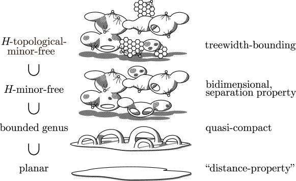
Figure 3: Kernelization results for problems with finite integer index on sparse graph classes with their corresponding additional condition.

The theorem that guarantees linear kernels on graphs of bounded genus in [7] imposes a condition called quasi-compactness. The notion of quasi-compactness is similar to that of treewidth-bounding: Yes-instances $(G,k)$ satisfy the condition that there exists a vertex set $X\subseteq V(G)$ of “small” size whose deletion yields a graph of bounded treewidth. Formally, a problem $\Pi$ is called quasi-compact if there exists an integer $r$ such that for every $(G,k)\in\Pi$, there is an embedding of $G$ onto a surface of Euler-genus at most $g$ and a set $X\subseteq V(G)$ such that $|X|\leqslant r\cdot k$ and $\mathop{\mathbf{missing}}{tw}(G-R^{r}_{G}(X))\leqslant r$. Here $R^{r}_{G}(X)$ denotes the set of vertices of $G$ at radial distance at most $r$ from $X$. It is easy to see that the property of being treewidth-bounding is stronger than quasi-compactness in the sense that if a problem is treewidth-bounding and the graphs are embeddable on a surface of genus $g$, then the problem is also quasi-compact, but not the other way around. The fact that we use a stronger structural condition is expected, since our result proves a linear kernel on a much larger graph class.

More interesting are the conditions imposed for linear kernels on $H$-minor-free graphs [37]. The problems here are required to be bidimensional and satisfy a so-called separation property. Roughly speaking, a problem is bidimensional if the solution size on a $k\times k$-grid is $\Omega(k^{2})$ and the solution size does not decrease by deleting/contracting edges. The notion of the separation property is essentially the following. A problem has the separation property, if for any graph $G$ and any vertex subset $X\subseteq V(G)$, the optimum solution of $G$ projected on any subgraph $G^{\prime}$ of $G-X$ differs from the optimum for $G^{\prime}$ by at most $|X|$ (cf. [37] for details.) At first glance, these conditions seem to have nothing to do with the property of being treewidth-bounding. However in the same paper [37, Lemma 3.2], the authors show that if a problem on $H$-minor-graphs is bidimensional and has the separation property then it is also $(ck,t)$-treewidth-bounding for some constants $c,t$ that depend on the graph $H$ excluded as a minor. Using this fact, the main result of [37] (namely, that bidimensional problems with FII and the separation property have linear kernels on $H$-minor-free graphs) can be reproved as an easy corollary of Theorem 1.

This discussion shows that in the results on linear kernels on sparse graph classes that we know so far, the treewidth-bounding condition has appeared in some form or the other. In the light of this we feel that this is the key condition for proving linear kernels on sparse graph classes.

4.3 The limits of our approach

It is interesting to know for which notions of sparseness (beyond $H$-topological-minor-free graphs) we can use our technique to obtain polynomial kernels. We show that our technique fails for the following notion of sparseness: graph classes that locally exclude a minor [22]. The notion of locally excluding a minor was introduced by Dawar et al. [22] and graphs that locally exclude a minor include bounded-genus graphs but are incomparable with $H$-minor-free graphs [63]. However we also show that there exists (restricted) graph classes that locally exclude a minor where it is still possible to obtain a polynomial kernel using our technique.

Definition 12 (Locally excluding a minor [22]).

A class $\mathcal{G}$ of graphs locally excludes a minor if for every $r\in\mathbb{N}$ there is a graph $H_{r}$ such that the $r$-neighborhood of a vertex of any graph of $\mathcal{G}$ excludes $H_{r}$ as a minor.

Therefore if $\mathcal{G}$ locally excludes a minor then the $1$-neighborhood of a vertex in any graph of $\mathcal{G}$ does not contain $H_{1}$ as a minor, and hence as a subgraph. In particular, the neighborhood of no vertex contains a clique on $h_{1}:=|H_{1}|$ vertices as a subgraph, meaning that the clique number of such graphs is bounded above by $h_{1}$. The total number of cliques in any graph of $\mathcal{G}$ is then bounded by $h_{1}n^{h_{1}}$, and the number of edges can be trivially bounded by $n^{2}$. We now have almost all the prerequisites for applying Theorem 1. However the class $\mathcal{G}$ is not closed under taking $d$-constrictions. Taking a $d$-constriction in a graph $G\in\mathcal{G}$ can increase the clique number of the constricted graph. This seems to be a bottleneck in applying Theorem 1. However if we assume that the size of the locally forbidden minors $\left\{H_{r}\right\}_{r\in\mathbb{N}}$ grows very slowly, then we can still obtain a polynomial kernel.

Definition 13.

Given $g\colon\mathbb{N}\rightarrow\mathbb{N}$, we say that a graph class $\mathcal{G}$ locally excludes minors according to $g$missing if there exists a constant $n_{0}\in\mathbb{N}$, such that for all $r\geqslant n_{0}$, the $g(r)$-neighborhood of a vertex in any graph of $\mathcal{G}$ does not contain $K_{r}$ as a minor.

Lemma 13.

Let $\mathcal{G}$ be a graph class that locally excludes a minor according to $g\colon\mathbb{N}\rightarrow\mathbb{N}$ and let $n_{0}$ be the constant as in the above definition. Then for any $r\geqslant n_{0}$, the class $\mathcal{G}$ $g(r)$-constricts into a graph class $\mathcal{H}$ that excludes $K_{r}$ as a subgraph.

Proof.

Assume the contrary. Let $G\in\mathcal{G}$ and suppose that for some $r\geqslant 2$ the graph $H$ obtained by a $g(r)$-constriction of $G$ contains $K_{r}$ as a subgraph. Pick any vertex $v$ in this subgraph of $H$. The $g(r)$-neighborhood of $v$ in $G$ must contain $K_{r}$ as a minor, a contradiction. ∎

Note that in the following, we assume that the problem is treewidth-bounding on general graphs.

Corollary 5.

Let $\Pi$ be a parameterized graph problem with finite integer index that is $(s(k),t_{\Pi})$-treewidth-bounding. Let $\mathcal{G}$ be a graph class locally excluding a minor according to a function $g\colon\mathbb{N}\rightarrow\mathbb{N}$ such that for all $r\geqslant n_{0}$, $g(r)\geqslant\rho^{\prime}(2t_{\Pi}+r)+1$. Then there exists a constant $r_{0}$ such that $\Pi$ admits kernels of size $O(s(k)^{r_{0}})$ on $\mathcal{G}$.

Proof.

By Lemma 13, taking a $g(r)$-constriction results in a graph class $\mathcal{H}$ that excludes $K_{r}$ as a subgraph, for large enough $r$. Fixing $r=n_{0}$, where $n_{0}$ is the constant in Definition 13, we apply Theorem 1 with the trivial functions $f_{E}(n)=n^{2}$, $f_{\#\omega}(n)=r\cdot n^{r}$ and $\omega_{\mathcal{H}}=r$. By Lemma 13, we have that $\omega_{\mathcal{G}_{H}}\leqslant r$. The kernel size is then bounded by

$$s(k)+s(k)^{2}2t+\left((s(k)+2t\cdot s(k)^{2})^{r}+s(k)+2t\cdot s(k)^{2}+1\right)\rho^{\prime}(2t+r)\in O(s(k)^{2r}),$$

where we omitted the subscript of $t_{\Pi}$ for the sake of readability. With $r_{0}=2r=2n_{0}$, the bound in the statement of the corollary follows. ∎

We do not know how quickly the function $\rho^{\prime}(\cdot)$ grows but intuition from automata theory seems to suggest that this has at least superexponential growth. As such, the graph class for which the polynomial kernel result holds (Corollary 5) is pretty restricted. However this does suggest a limit to which our approach can be pushed as well as some intuition as to why our result is not easily extendable to graph classes locally excluding a minor. We note that graph classes of bounded expansion present the same problem.

4.4 An illustrative example: Edge Dominating Set

In this section we show how Theorem I can actually be used to obtain a simple explicit kernel for the Edge Dominating Set problem on $H$-topological-minor-free graphs. This is made possible by the fact that we can find in polynomial time a small enough treewidth-modulator and replace the generic protrusion reduction rule by a handcrafted specific reduction rule.

Let us first recall the problem at hand. We say that an edge $e$ is dominated by a set of edges $D$ if either $e\in D$ or $e$ is incident with at least one edge in $D$. The problem Edge Dominating Set asks, given a graph $G$ and an integer $k$, whether there is an edge dominating set $D\subseteq E(G)$ of size at most $k$, i.e., an edge set which dominates every edge of $G$. The canonical parameterization of this problem is by the integer $k$, i.e. the size of solution set.

There is a simple 2-approximation algorithm for Edge Dominating Set [73]. Given an instance $(G,k)$, where G is $H$-topological-minor-free, let $D$ be an edge dominating set of $G$, given by the 2-approximation. We can assume that $|D|\leqslant 2k$ since otherwise we can correctly declare $(G,k)$ as a No-instance. Take $X:=\{v\in V(G)\mid v\text{ is incident to some edge in }D\}$ as the treewidth-modulator: note that $|X|\leqslant 4k$ and that $G-X$ is of treewidth at most $0$, i.e., an independent set. One can easily verify that that the bag marking Algorithm 1 of Section 3 would mark exactly those vertices of $G-X$ whose neighborhood in $X$ has size at least $r:=|H|$. By applying the edge-bound of Proposition 2 to Lemma 11 we get that $|V(\mathcal{M})|\leqslant\beta r^{2}\cdot 8k$.

Take $Y_{0}:=X\cup V(\mathcal{M})$ and let $\mathcal{P}:=Y_{0}\uplus Y_{1}\uplus\cdots\uplus Y_{\ell}$ be a partition of $V(G)$, where again $Y_{i}$, $1\leqslant i\leqslant q$, is now a cluster w.r.t. $Y_{0}$, i.e. the vertices in a single $Y_{i}$ share the same neighborhood in $X$ and the $Y_{i}$ are of maximal size under this condition. We have one reduction rule, which can be construed as an concrete instantiation of generic the protrusion replacement rule. We would like to stress that this reduction rule relies on the fact that we already have a protrusion decomposition of $G$, given by Algorithm 1.

Twin elimination rule: If $|Y_{i}|>|N_{Y_{0}}(Y_{i})|$ for some $i\neq 0$, let $G^{\prime}$ be the instance obtained by keeping $|N_{Y_{0}}(Y_{i})|$ many vertices of $Y_{i}$ and removing the rest of $Y_{i}$. Take $k^{\prime}:=k$.

Lemma 14.

The twin elimination rule is safe.

Proof.

Let $G_{i}$ be the graph induced by the vertex set $N_{Y_{0}}(Y_{i})\cup Y_{i}$ and let $E_{i}$ be its edge set (as $N_{Y_{0}}(Y_{i})=N(Y_{i})$, we shall omit the subscript $Y_{0}$). For a vertex $v\in V(G)$, we define the set $E(v)$ as the set of edges incident with $v$. The notations $G^{\prime}_{i}$, $E^{\prime}_{i}$, $Y^{\prime}_{i}$, and $E^{\prime}(v)$ are defined analogously for the graph $G^{\prime}$ obtained after the application of twin elimination rule. We say that a vertex $v\in V(G)$ is covered by an edge set $D$ if $v$ is incident with an edge of $D$.

To see the forward direction, suppose that $(G,k)$ is a Yes-instance and let $D$ be an edge dominating set of size at most $k$. Without loss of generality, we can assume that $|D\cap E_{i}|\leqslant|N(Y_{i})|$. Indeed, it can be easily checked that the edge set $(D\setminus E_{i})\cup E(u)$, for an arbitrarily chosen $u\in Y_{i}$, is an edge dominating set. Hence at most $|N(Y_{i})|$ vertices out of $Y_{i}$ are covered by $D$, and thus we can apply twin elimination rule so as to delete only those vertices which are not incident with $D$. It just remains to observe that $D$ is an edge dominating set of $G^{\prime}$.

For the opposite direction, let $D^{\prime}$ be an edge dominating set for $G^{\prime}$ of size at most $k$. We first argue that $N(Y^{\prime}_{i})$ is covered by $D^{\prime}$ without loss of generality. Indeed, suppose $v\in N(Y^{\prime}_{i})$ is not covered by $D^{\prime}$. In order for an edge $e=uv\in E^{\prime}(v)\cap E^{\prime}_{i}$ to be dominated by $D^{\prime}$, at least one edge in $E^{\prime}(u)$ should be contained in $D$. Since the sets $\{E^{\prime}(u):u\in Y^{\prime}_{i}\}$ are mutually disjoint, it follows that $|D^{\prime}\cap E^{\prime}_{i}|\geqslant|Y^{\prime}_{i}|$. Now take an alternative edge set $D^{\prime\prime}:=(D^{\prime}\setminus E^{\prime}_{i})\cup E^{\prime}(u)$ for an arbitrary vertex $u\in Y^{\prime}_{i}$. It is not difficult to see that $D^{\prime\prime}$ is an edge dominating set for $G^{\prime}$. Moreover, we have $|D^{\prime\prime}|\leqslant|D^{\prime}|\leqslant k$ as $|D^{\prime}\cap E^{\prime}_{i}|\geqslant|Y^{\prime}_{i}|=|E^{\prime}(u)|=|N(Y^{\prime}_{i})|$. Hence $D^{\prime\prime}$ is also an edge dominating set of size at most $k$. Assuming that $N(Y^{\prime}_{i})$ is covered by $D^{\prime}$, it is easy to see that $D^{\prime}$ dominates $E_{i}$ and thus $D^{\prime}$ is an edge dominating set of $G$. This complete the proof. ∎

Back to the partition $\mathcal{P}$, we can apply twin elimination rule in time $O(n)$ and ensure that $|Z_{i}|\leqslant r-1$ for $1\leqslant i\leqslant q$. The bound on $q$ is proved in Lemma 12 and taken together with the edge- and clique-bounds from Proposition 2 and 3, respectively, we obtain

$$q\leqslant 2^{\tau r\log r}((2\beta r^{2}+1)4k)+(2\beta r^{2}+1)4k+1$$

and thus we get the overall bound

$$|G| \leqslant |Y_{0}|+|Y_{1}|+\dots+|Y_{q}|$$

$$= (2\beta r^{2}+1)4k+(2^{\tau r\log r}((2\beta r^{2}+1)4k)+((2\beta r^{2}+1)4k)+1)(r-1)$$

$$= 4k\left(1+2\beta r^{2}+(2^{\tau r\log r+1}\beta r^{2}+2^{\tau r\log r}+2\beta r^{2})(r-1)\right)+r-1$$

$$< 4k\left(1+20r^{2}+(20.8^{r\log r+1}20r^{2}+20.8^{r\log r}+20r^{2})(r-1)\right)+r$$

on the size of $G$. We remark that this upper bound can be easily made explicit once $H$ is fixed. Again, we can get better constants on $H$-minor-free graphs, just by replacing constants $\beta r^{2}$ and $2^{\tau r\log r}$ with $\alpha(r\sqrt{\log r})$ and $2^{\mu r\log\log r}$, respectively. Finally, note that the whole procedure can be carried out in linear time.

5 Single-exponential algorithm for Planar-$\mathcal{F}$-Deletion

This section is devoted to the single-exponential algorithm for the Planar-$\mathcal{F}$-Deletion problem. Let henceforth $H_{p}$ be some fixed (connected or disconnected) arbitrary planar graph in the family $\mathcal{F}$, and let $r:=|H_{p}|$. First of all, using iterative compression, we reduce the problem to obtaining a single-exponential algorithm for the Disjoint Planar-$\mathcal{F}$-Deletion problem, which is defined as follows:

Disjoint Planar-$\mathcal{F}$-Deletion
Input:	A graph $G$ and a subset of vertices $X\subseteq V(G)$ such that $G-X$ is $H$-minor-free for every $H\in\mathcal{F}$.
Parameter:	The integer $k=|X|$.
Objective:	Compute a set $\tilde{X}\subseteq V(G)$ disjoint from $X$ such that $|\tilde{X}|<|X|$ and $G-\tilde{X}$ is $H$-minor-free for every $H\in\mathcal{F}$, if such a set exists.

The input set $X$ is called the initial solution and the set $\tilde{X}$ the alternative solution. Let $t_{\mathcal{F}}$ be a constant (depending on the family $\mathcal{F}$) such that $\mathop{\mathbf{missing}}{tw}(G-X)\leqslant t_{\mathcal{F}}-1$ (note that such a constant exists by Robertson and Seymour [67]).

The following lemma relies on the fact that being $\mathcal{F}$-minor-free is a hereditary property with respect to induced subgraphs. We omit the proof as it is now a classical statement (the interested reader can refer, for example, to [17, 57, 45, 48]).

Lemma 15.

If the parameterized Disjoint Planar-$\mathcal{F}$-Deletion problem can be solved in time $c^{k}\cdot p(n)$, where $c$ is a constant and $p(n)$ is a polynomial in $n$, then the parameterized Planar-$\mathcal{F}$-Deletion problem can be solved in time $(c+1)^{k}\cdot p(n)\cdot n$.

Let us provide a brief sketch of our algorithm to solve Disjoint Planar-$\mathcal{F}$-Deletion. We start by computing a protrusion decomposition using Algorithm 1 with input $(G,X,r)$. But it turns out that the set $Y_{0}$ output by Algorithm 1 does not define a linear protrusion decomposition of $G$, which is crucial for our purposes (in fact, it can be only proved that $Y_{0}$ defines a quadratic protrusion decomposition of $G$). To circumvent this problem, our strategy is to first use Algorithm 1 to identify a set $Y_{0}$ of $O(k)$ vertices of $G$, and then guess the intersection $I$ of the alternative solution $\tilde{X}$ with the set $Y_{0}$. We prove that if the input is a Yes-instance of Disjoint Planar-$\mathcal{F}$-Deletion, then $V(\mathcal{M})$ contains a subset $I$ such that the connected components of $G-V(\mathcal{M})$ can be clustered together with respect to their neighborhood in $Y_{0}\setminus I$ to form an $(O(k-|I|),2t_{\mathcal{F}}+r)$-protrusion decomposition $\mathcal{P}$ of the graph $G-I$. As a result, we obtain Proposition 5, which is fundamental in order to prove Theorem II.

Proposition 5 (Linear protrusion decomposition).

Let $(G,X,k)$ be a Yes-instance of the parameterized Disjoint Planar-$\mathcal{F}$-Deletion problem. There exists a $2^{O(k)}\cdot n$-time algorithm that identifies a set $I\subseteq V(G)$ of size at most $k$ and a $(O(k),2t_{\mathcal{F}}+r)$-protrusion decomposition $\mathcal{P}=Y_{0}\uplus Y_{1}\uplus\cdots\uplus Y_{\ell}$ of $G-I$ such that:

1. $X\subseteq Y_{0}$;

2. there exists a set $X^{\prime}\subseteq V(G)\setminus Y_{0}$ of size at most $k-|I|$ such that $G-\tilde{X}$, with $\tilde{X}=X^{\prime}\cup I$, is $H$-minor-free for every graph $H\in\mathcal{F}$.

At this stage of the algorithm, we can assume that a subset $I$ of the alternative solution $\tilde{X}$ has been identified, and it remains to solve the instance $(G-I,X,k-|I|)$ of the Disjoint Planar-$\mathcal{F}$-Deletion problem, which comes equipped with a linear protrusion decomposition $\mathcal{P}=Y_{0}\uplus Y_{1}\uplus\cdots\uplus Y_{\ell}$. In order to solve this problem, we prove the following proposition:

Proposition 6.

Let $(G,Y_{0},k)$ be an instance of Disjoint Planar-$\mathcal{F}$-Deletion and let $\mathcal{P}=Y_{0}\uplus Y_{1}\uplus\cdots\uplus Y_{\ell}$ be an $(\alpha,\beta)$-protrusion decomposition of $G$, for some constant $\beta$. There exists an $2^{O(\ell)}\cdot n$-time algorithm which computes a solution $\tilde{X}\subseteq V(G)\setminus Y_{0}$ of size at most $k$ if it exists, or correctly decides that there is no such solution.

The key observation in the proof of Proposition 6 is that for every restricted protrusion $Y_{i}$, there is a finite number of representatives such that any partial solution lying on $Y_{i}$ can be replaced with one of them while preserving the feasibility of the solution. This follows from the finite index of MSO-definable properties (see, e.g., [11]). Then, to solve the problem in single-exponential time we can just use brute-force in the union of these representatives, which has overall size $O(k)$.

Organization of the section.

In Subsection 5.1 we analyze Algorithm 1 when the input graph is a Yes-instance of Disjoint Planar-$\mathcal{F}$-Deletion. The branching step guessing the intersection of the alternative solution $\tilde{X}$ with $V(\mathcal{M})$ is described in Subsection 5.2, concluding the proof of Proposition 5. Subsection 5.3 gives a proof of Proposition 6, and finally Subsection 5.4 proves Theorem II.

5.1 Analysis of the bag marking algorithm

We first need two results concerning graphs with excluding clique minor. The following lemma states that graphs excluding a fixed graph as a minor have linear number of edges.

Proposition 7 (Thomason [72]).

There is a constant $\alpha<0.320$ such that every $n$-vertex graph with no $K_{r}$-minor has at most $(\alpha r\sqrt{\log r})\cdot n$ edges.

Recall that a clique in a graph is a set of pairwise adjacent vertices. For simplicity, we assume that a single vertex and the empty graph are also cliques.

Proposition 8 (Fomin, Oum, and Thilikos [39]).

There is a constant $\mu<11.355$ such that, for $r>2$, every $n$-vertex graph with no $K_{r}$-minor has at most $2^{\mu r\log\log r}\cdot n$ cliques.

For the sake of simplicity, let henceforth in this section $\alpha_{r}:=\alpha r\sqrt{\log r}$ and $\mu_{r}:=2^{\mu r\log\log r}$.

Let us now analyze some properties of Algorithm 1 when the input graph is a Yes-instance of the Disjoint Planar-$\mathcal{F}$-Deletion problem. In this case, the bound on the treewidth of $G-X$ is $t_{\mathcal{F}}-1$. The following two lemmas show that the number of bags identified at the “Large-subgraph marking step” is linearly bounded by $k$. Their proofs use arguments similar to those used in the proof of Theorem 1, but we provide the full proofs here for completeness.

Lemma 16.

Let $(G,X,k)$ be a Yes-instance of the Disjoint Planar-$\mathcal{F}$-Deletion problem. If $C_{1},\ldots,C_{\ell}$ is a collection of connected pairwise disjoint subsets of $V(G)\setminus X$ such that for all $1\leqslant i\leqslant\ell$, $|N_{X}(C_{i})|\geqslant r$, then $\ell\leqslant(1+\alpha_{r})\cdot k$.

Proof.

Let $X^{\prime}\subseteq V(G)\setminus X$ be a solution for $(G,X,k)$, and observe that $\ell^{\prime}\leqslant k$ of the sets $C_{1},\ldots,C_{\ell}$ contain vertices of $X^{\prime}$. Consider the sets $C_{\ell^{\prime}+1},\dots,C_{\ell}$ which are disjoint with $X^{\prime}$, and observe that $G[X\cup(\bigcup_{\ell^{\prime}<j\leqslant\ell}C_{j})]$ is an $H$-minor-free graph. We proceed to construct a family of graphs $\{G_{i}\}_{\ell^{\prime}\leqslant i\leqslant\ell}$, with $V(G_{i})=X$ for all $\ell^{\prime}\leqslant i\leqslant\ell$, and such that $G_{i}$ is a minor of $G[X\cup(\bigcup_{\ell^{\prime}<j\leqslant i}C_{j})]$, in the following way. We start with $E(G_{\ell^{\prime}})=E[G(X)]$, and suppose inductively that the graph $G_{i-1}$ has been successfully constructed. Since by assumption $G_{i-1}$ is a minor of $G[X\cup(\bigcup_{\ell^{\prime}<j\leqslant i-1}C_{j})]$, which in turn is a minor of $G[X\cup(\bigcup_{\ell^{\prime}<j\leqslant\ell}C_{j})]$, it follows that $G_{i-1}$ is $H$-minor-free, and therefore it cannot contain a clique on $r$ vertices. In order to construct $G_{i}$ from $G_{i-1}$, let $x_{i},y_{i}$ be two vertices in $X$ such that both $x_{i}$ and $y_{i}$ are neighbors in $G$ of some vertex in $C_{i}$, and such that $x_{i}$ and $y_{i}$ are non-adjacent in $G_{i-1}$. Note that such two vertices exist, since we can assume that $r\geqslant 2$ and $G_{i-1}$ is $H$-minor-free. Then $G_{i}$ is constructed from $G_{i-1}$ by adding an edge between $x_{i}$ and $y_{i}$. Since $C_{i}$ is connected by hypothesis, we have that $G_{i}$ is indeed a minor of $G[X\cup(\bigcup_{\ell^{\prime}<j\leqslant i}C_{j})]$. Since $G_{\ell}$ is $H$-minor-free, it follows by Proposition 7 that $|E(G_{\ell})|\leqslant\alpha_{r}\cdot|X|$ edges. Since by construction we have that $\ell-\ell^{\prime}\leqslant|E(G_{\ell})|$, we conclude that $\ell=\ell^{\prime}+(\ell-\ell^{\prime})\leqslant k+\alpha_{r}\cdot k=(1+\alpha_{r})\cdot k$, as we wanted to prove.∎

Lemma 17.

If $(G,X,k)$ is a Yes-instance of the Disjoint Planar-$\mathcal{F}$-Deletion problem, then the set $Y_{0}=V(\mathcal{M})\cup X$ of vertices returned by Algorithm 1 has size at most $k+2t_{\mathcal{F}}\cdot(1+\alpha_{r})\cdot k$.

Proof.

As $|X|=k$ and as the algorithm marks bags of an optimal forest-decomposition of $G-X$, which is a graph of treewidth at most $t_{\mathcal{F}}$, in order to prove the lemma it is enough to prove that the number of marked bags is at most $2\cdot(1+\alpha_{r})\cdot k$. It is an easy observation to see that the set of connected components $C_{B}$ identified at the Large-subgraph marking step contains pairwise vertex disjoint subset of vertices, each inducing a connected subgraph of $G-X$ with at least $r$ neighbors in $X$. It follows by Lemma 16, that the number of bags marked at the Large-subgraph marking step is at most $(1+\alpha_{r})\cdot k$. To conclude it suffices to observe that the number of bags identified at the LCA marking step cannot exceed the number of bags marked at the Large-subgraph marking step. ∎

5.2 Branching step and linear protrusion decomposition

At this stage of the algorithm, we have identified a set $Y_{0}=X\cup V(\mathcal{M})$ of $O(k)$ vertices such that, by Proposition 1, every connected component of $G-Y_{0}$ is a restricted $(2t_{\mathcal{F}}+r)$-protrusion. We would like to note that it can be proved, using ideas similar to the proof of Lemma 18 below, that $Y_{0}$ together with the clusters of $G-Y_{0}$ form a quadratic protrusion decomposition of the input graph $G$. But as announced earlier, for time complexity issues we seek a linear protrusion decomposition. To this end, the second step of the algorithm consists in a branching to guess the intersection $I$ of the alternative solution $\tilde{X}$ with the set of marked vertices $V(\mathcal{M})$. By Lemma 17, this step yields $2^{O(k)}$ branchings, which is compatible with the desired single-exponential time.

For each guessed set $I\subseteq Y_{0}$, we denote $G_{I}:=G-I$. Recall that a cluster of $G_{I}-Y_{0}$ as a maximal collection of connected components of $G_{I}-Y_{0}$ with the same neighborhood in $Y_{0}\setminus I$. We use Observation 2, a direct consequence of Lemma 8, to bound the number of clusters under the condition that $G_{I}$ contains a vertex subset $X^{\prime}$ disjoint from $Y_{0}$ of size at most $k-|I|$ such that $G_{I}-X^{\prime}$ does not contain any graph $H\in\mathcal{F}$ as a minor (and so the graph $G-\tilde{X}$, with $\tilde{X}=X^{\prime}\cup I$, does not contain either any graph $H\in\mathcal{F}$ as a minor).

Observation 2.

For every cluster $\mathcal{C}$ of $G_{I}-Y_{0}$, $|N_{Y_{0}}(\mathcal{C})|<r+2t_{\mathcal{F}}$.

The proof of the following lemma has a similar flavor to those of Theorem 1 and Lemma 16.

Lemma 18.

If $(G_{I},Y_{0}\setminus I,k-|I|)$ is a Yes-instance of the Disjoint Planar-$\mathcal{F}$-Deletion problem, then the number of clusters of $G_{I}-Y_{0}$ is at most $(5t_{\mathcal{F}}\alpha_{r}\mu_{r})\cdot k$.

Proof.

Let $\mathcal{C}$ be the collection of all clusters of $G_{I}-Y_{0}$. Let $X^{\prime}$ be a subset of vertices disjoint from $Y_{0}$ such that $|X^{\prime}|\leqslant k-|I|=k_{I}$ and $G_{I}-X^{\prime}$ is $H$-minor-free for every graph $H\in\mathcal{F}$. Observe that at most $k_{I}$ clusters in $\mathcal{C}$ contain vertices from $X^{\prime}$. Let $C_{1},\ldots,C_{\ell}$ be the clusters in $\mathcal{C}$ that do not contain vertices from $X^{\prime}$. So we have that $|\mathcal{C}|\leqslant k_{I}+\ell\leqslant k+\ell$. Let $G_{\mathcal{C}}$ be the subgraph of $G$ induced by $(Y_{0}\setminus I)\cup\bigcup_{i=1}^{\ell}C_{i}$. Observe that as $(G_{I},Y_{0}\setminus I,k-|I|)$ is a Yes-instance of the Disjoint Planar-$\mathcal{F}$-Deletion problem, $G_{\mathcal{C}}$ is $H$-minor-free for every graph $H\in\mathcal{F}$.

We greedily construct from $G_{\mathcal{C}}$ a graph $G_{\mathcal{C}}^{\prime}$, with $V(G_{\mathcal{C}}^{\prime})=Y_{0}\setminus I$, as follows. We start with $G_{\mathcal{C}}^{\prime}=G[Y_{0}\setminus I]$. As long as there is a non-used cluster $C\in\mathcal{C}$ with two non-adjacent neighbors $u,v$ in $Y_{0}\setminus I$, we add to $G_{\mathcal{C}}^{\prime}$ an edge between $u$ and $v$ and mark $C$ as used. The number of clusters in $\mathcal{C}$ used so far in the construction of $G_{\mathcal{C}}^{\prime}$ is bounded above by the number of edges of $G_{\mathcal{C}}^{\prime}$. Observe that by construction $G_{\mathcal{C}}^{\prime}$ is clearly a minor of $G_{\mathcal{C}}$. Thereby $G^{\prime}_{\mathcal{C}}$ is an $H$-minor-free graph (for every $H\in\mathcal{F}$) on at most $k+2t_{\mathcal{F}}\cdot(1+\alpha_{r})\cdot k$ vertices (by Lemma 17). By Proposition 7, it follows that $|E(G_{\mathcal{C}}^{\prime})|\leqslant\alpha_{r}\cdot(k+2t_{\mathcal{F}}\cdot(1+\alpha_{r})\cdot k)$ and so there are the same number of used clusters.

Let us now count the number of non-used clusters. Observe that the neighborhood in $Y_{0}\setminus I$ of each non-used cluster induces a (possibly empty) clique in $G_{\mathcal{C}}^{\prime}$ (as otherwise some further edge could have been added to $G_{\mathcal{C}}^{\prime}$). As by definition distinct clusters have distinct neighborhoods in $Y_{0}\setminus I$, and as $G_{\mathcal{C}}^{\prime}$ is an $H$-minor-free graph (for every $H\in\mathcal{F}$) on at most $k+2t_{\mathcal{F}}\cdot(1+\alpha_{r})\cdot k$ vertices, Proposition 8 implies that the number of non-used clusters is at most $\mu_{r}\cdot(k+2t_{\mathcal{F}}\cdot(1+\alpha_{r})\cdot k)$. Summarizing, we have that $|\mathcal{C}|\leqslant k+(\alpha_{r}+\mu_{r})\cdot(k+2t_{\mathcal{F}}\cdot(1+\alpha_{r})\cdot k)\leqslant(5t_{\mathcal{F}}\alpha_{r}\mu_{r})\cdot k$, where in the last inequality we have used that $\mu_{r}\geqslant\alpha_{r}$ and we have assumed that $\alpha_{r}\geqslant 4$. ∎

Piecing all lemmas together, we can now provide a proof of Proposition 5.

Proof of Proposition 5.

By Lemmas 6 and 17 and Observation 2, we can compute in linear time a set $Y_{0}$ of $O(k)$ vertices containing $X$ such that every cluster of $G-Y_{0}$ is a restricted $(2t_{\mathcal{F}}+r)$-protrusion. If $(G,X,k)$ is a Yes-instance of the Disjoint Planar-$\mathcal{F}$-Deletion problem, then there exists a set $\tilde{X}$ of size at most $|X|$ and disjoint from $X$ such that $G-\tilde{X}$ does not contain any graph $H\in\mathcal{F}$ as a minor. Branching on every possible subset of $Y_{0}\setminus X$, one can guess the intersection $I$ of $\tilde{X}$ with $Y_{0}\setminus X$. By Lemma 17, the branching degree is $2^{O(k)}$. As $(G,X,k)$ is a Yes-instance, for at least one of the guessed subsets $I$, the instance $(G_{I},Y_{0}\setminus I,k-|I|)$ is a Yes-instance of the Disjoint Planar-$\mathcal{F}$-Deletion problem. By Lemma 18, the partition $\mathcal{P}=(Y_{0}\setminus I)\uplus Y_{1}\uplus\cdots\uplus Y_{\ell}$, where $\{Y_{1},\dots,Y_{\ell}\}$ is the set of clusters of $G_{I}-Y_{0}$, is an $(O(k),r+2t_{\mathcal{F}})$-protrusion decomposition of $G_{I}$. ∎

5.3 Solving Planar-F-Deletion with a linear protrusion decomposition

After having proved Proposition 5, we can now focus in this subsection on solving Disjoint Planar-$\mathcal{F}$-Deletion in single-exponential time when a linear protrusion decomposition is given. Let $P_{\Pi}(G,S)$ denote the MSO formula which holds if and only if $G-S$ is $\mathcal{F}$-minor-free.

Consider an instance $(G,Y_{0},k)$ of Disjoint Planar-$\mathcal{F}$-Deletion equipped with a linear protrusion decomposition $\mathcal{P}$ of $G$. Let $\mathcal{P}=Y_{0}\uplus Y_{1}\uplus\cdots\uplus Y_{\ell}$ be an $(\alpha,\beta)$-protrusion decomposition of $G$ for some constant $\beta$. The key observation is that for every restricted protrusion $Y_{i}$, there is a finite number of representatives such that any partial solution lying on $Y_{i}$ can be replaced with one of them while preserving the feasibility of the solution.

We fix a constant $t$. Let $\mathcal{U}_{t}$ be the universe of $t$-boundaried graphs, and let $\mathcal{U}_{t}^{\mbox{{\tiny small}}}$ denote the universe of $t$-boundaried graphs with treewidth at most $t-1$. Throughout this subsection we will assume that all the restricted protrusions belonging to a given protrusion decomposition have the same boundary size, equal to the maximum boundary size over all protrusions. This assumption is licit as if some protrusion has smaller boundary size, we can add dummy independent vertices to it without interfering with the structure of the solutions and without increasing the treewidth.

Definition 14.

Let $\mathcal{P}=Y_{0}\uplus Y_{1}\uplus\cdots\uplus Y_{\ell}$ be an $(\alpha,t)$-protrusion decomposition of $G$. For each $1\leqslant i\leqslant\ell$, we define the following equivalence relation $\sim_{\mathcal{F},i}$ on subsets of $Y_{i}$: for $Q_{1},Q_{2}\subseteq Y_{i}$, we define $Q_{1}\sim_{\mathcal{F},i}Q_{2}$ if for every $H\in\mathcal{U}_{t}$, $G[Y_{i}^{+}\setminus Q_{1}]\oplus H$ is $\mathcal{F}$-minor-free if and only if $G[Y_{i}^{+}\setminus Q_{2}]\oplus H$ is $\mathcal{F}$-minor-free.

Note that $G$ equipped with $\mathcal{P}$ can be viewed as a gluing of two $\beta$-boundaried graphs $G[Y_{i}^{+}]$ and $G\ominus G[Y_{i}^{+}]$, for any $1\leqslant i\leqslant\ell$, where $Y_{i}^{+}=N_{G_{I}}[Y_{i}]$. Let us consider the equivalence relation $\sim_{\mathcal{F},i}$ applied on $Y_{i}$ when $G$ is viewed as such gluing. Extending the notation suggested in Section 2, we say that $\mathcal{S}$ is a set of (minimum-sized) representatives of the equivalence relation $\approx$ if $\mathcal{S}$ contains exactly one element (of minimum cardinality) from every equivalence class under $\approx$. Let $\mathcal{R}(Y_{i}):=\{Q^{i}_{1},\ldots,Q^{i}_{q_{i}}\}$ be a set of minimum-sized representatives of equivalence classes under $\sim_{\mathcal{F},i}$ for every $1\leqslant i\leqslant\ell$. We say that a set $\tilde{X}\subseteq V(G)\setminus Y_{0}$ is decomposable if $\tilde{X}=Q^{1}\cup\cdots\cup Q^{\ell}$ for some $Q^{i}\in\mathcal{R}(Y_{i})$ for $1\leqslant i\leqslant\ell$.

Lemma 19 (Solution decomposability).

Let $(G,Y_{0},k)$ be an instance of Disjoint Planar-$\mathcal{F}$-Deletion and let $\mathcal{P}=Y_{0}\uplus Y_{1}\uplus\cdots\uplus Y_{\ell}$ be an $(\alpha,\beta)$-protrusion decomposition of $G$. Then, there exists a solution $\tilde{X}\subseteq V(G)\setminus Y_{0}$ of size at most $k$ if and only if there exists a decomposable solution $\tilde{X}^{*}\subseteq V(G)\setminus Y_{0}$ of size at most $k$.

Proof.

Let $\tilde{X}$ be a subset of $V(G)\setminus Y_{0}$. Let $S_{i}:=\tilde{X}\cap Y_{i}$ for every $1\leqslant i\leqslant\ell$, $\bar{S}_{i}:=\tilde{X}\cap(V(G)\setminus Y_{i})$ and let $H:=G\ominus G[Y_{i}^{+}]-\bar{S}_{i}$ be the associated $t$-boundaried graph with $\mathop{\mathbf{missing}}{bd}(H):=\mathop{\mathbf{missing}}{bd}(G\ominus G[Y_{i}^{+}])$. Fix $i$ and choose the (unique) representative $Q^{i}\in\mathcal{R}(Y_{i})$ such that $Q^{i}\sim_{\mathcal{F},i}S_{i}$. Note that $S_{i}\cap\mathop{\mathbf{missing}}{bd}(H)=\bar{S}_{i}\cap\mathop{\mathbf{missing}}{bd}(H)=\emptyset$.

We claim that $G-\tilde{X}$ is $\mathcal{F}$-minor-free if and only if $G-(Q^{i}\cup\bar{S}_{i})$ is $\mathcal{F}$-minor-free. Indeed, $G-\tilde{X}=G-(S_{i}\cup\bar{S}_{i})$, which can be written as $G[Y_{i}^{+}\setminus S_{i}]\oplus H$. From the choice of $Q^{i}\in\mathcal{R}(Y_{i})$ such that $Q^{i}\sim_{\mathcal{F},i}S_{i}$, it follows that $G[Y_{i}^{+}\setminus S_{i}]\oplus H$ is $\mathcal{F}$-minor-free if and only if $G[Y_{i}^{+}\setminus Q^{i}]\oplus H$ is so. Noting that $G[Y_{i}^{+}\setminus Q^{i}]\oplus H=G-(Q^{i}\cup\bar{S}_{i})$ proves our claim.

By replacing each $S_{i}$ with its representative $Q^{i}\in\mathcal{R}(Y_{i})$, we eventually obtain $\tilde{X}^{*}$ of the form $\tilde{X}^{*}=\bigcup_{1\leqslant i\leqslant\ell}Q^{i}$, where $Q^{i}\in\mathcal{R}(Y_{i})$ is the representative of $S_{i}$ for every $1\leqslant i\leqslant\ell$. Finally, it holds that $P_{\Pi}(G,\tilde{X}^{*})$ if and only if $P_{\Pi}(G,\tilde{X})$. It remains to observe that $|Q^{i}|\leqslant|S_{i}|$, as we selected a minimum-sized set of an equivalence class of $\sim_{\mathcal{F},i}$ as its representative. ∎

We are now ready to prove Proposition 6.

Reminder of Proposition 6. Let $(G,Y_{0},k)$ be an instance of Disjoint Planar-$\mathcal{F}$-Deletion and let $\mathcal{P}=Y_{0}\uplus Y_{1}\uplus\cdots\uplus Y_{\ell}$ be an $(\alpha,\beta)$-protrusion decomposition of $G$, for some constant $\beta$. There exists an $2^{O(\ell)}\cdot n$-time algorithm which computes a solution $\tilde{X}\subseteq V(G)\setminus Y_{0}$ of size at most $k$ if it exists, or correctly decides that there is no such solution.

Proof.

By Lemma 19, either there exists a solution of size at most $k$ which is decomposable or $(G,Y_{0},k)$ is a No-instance. Assume that the representatives $\mathcal{R}(Y_{i})$ of the equivalence relations $\sim_{\mathcal{F},i}$ are given for all $1\leqslant i\leqslant\ell$. Then, for a decomposable set $\tilde{X}$, one can decide if $\tilde{X}$ is a solution or not in time $O(h(t_{\mathcal{F}})\cdot n)$. Indeed, for $\tilde{X}$ to be a solution, the treewidth of $G-\tilde{X}$ is at most $t_{\mathcal{F}}-1$. Using the algorithm of Bodlaender [6], one can decide in time $2^{O(t_{\mathcal{F}}^{3})}\cdot n$ whether a graph is of treewidth at most $t_{\mathcal{F}}$ and if so, build a tree-decomposition of width at most $t_{\mathcal{F}}$. Courcelle’s theorem [18] says that testing an MSO-definable property on treewidth-$t_{\mathcal{F}}$ graphs can be done in linear time, where the hidden constant depends solely on the treewidth $t_{\mathcal{F}}$ and the length of the MSO-sentence. It follows that one can decide whether $G-\tilde{X}$ is $\mathcal{F}$-minor-free or not in time $O(h(t_{\mathcal{F}})\cdot n)$. Here $h(t_{\mathcal{F}})$ is an additive function resulting from Bodlaender’s treewidth testing algorithm and Courcelle’s MSO-model checking algorithm, which depends solely on the treewidth $t_{\mathcal{F}}$ and the MSO formula $|P_{\Pi}(G,\tilde{X})|$. It remains to observe that there are at most $2^{O(\ell)}$ decomposable sets to consider. This is because an MSO-definable graph property has finitely many equivalence classes on $\mathcal{U}_{t}$ for every fixed $t$ [18, 11] (hence, also on $\mathcal{U}_{t}^{\mbox{{\tiny small}}}$), and being $\mathcal{F}$-minor-free is an MSO-definable property. ∎

Constructing the sets of representatives.

We remark that in the proof of Proposition 6 we have assumed that the sets of representatives $\mathcal{R}(Y_{i})$ are given to the algorithm. This makes the algorithm of Proposition 6 (and therefore, also the algorithm of Theorem II) non-constructive, and uniform on $k$ but non-uniform on the family $\mathcal{F}$. That is, for each family $\mathcal{F}$ we deduce the existence of a different algorithm. In order to make our algorithms constructive and uniform also on $\mathcal{F}$, we now proceed to explain how to construct the minimum-sized sets of representatives $\mathcal{R}(Y_{i})$ in linear time .

Our strategy can be summarized as follows. We will first define an equivalence relation $\equiv_{\mathcal{F},t}$ on $\mathcal{U}_{t}^{\mbox{{\tiny small}}}$, with the objective of capturing all possible behaviors of the graphs $G\ominus G[Y_{i}^{+}]$ (we call such graphs the context of the restricted protrusion $Y_{i}$). From classic tree automaton theory [29, 19], Courcelle’s theorem [18], and the fact that $\equiv_{\mathcal{F},t}$ has finitely many equivalence classes for each fixed $t$, it follows that a finite set $\mathcal{K}$ of representatives of $\equiv_{\mathcal{F},t}$ can be efficiently computed in constant time. Once we have the set $\mathcal{K}$, we compute our desired set $\mathcal{R}(Y_{i})$ in each restricted protrusion $Y_{i}$ by solving a constant number of $p$-min-CMSO graph problems on graphs of bounded treewidth, using the dynamic programming linear-time algorithm of Borie et al. [13]. The details follow.

For two $t$-boundaried graphs $K_{1}$ and $K_{2}$ from $\mathcal{U}_{t}^{\mbox{{\tiny small}}}$, we say that $K_{1}\equiv_{\mathcal{F},t}K_{2}$ if for every $Y\in\mathcal{U}_{t}^{\mbox{{\tiny small}}}$, $K_{1}\oplus Y$ is $\mathcal{F}$-minor-free iff $K_{2}\oplus Y$ is $\mathcal{F}$-minor-free. The intuition is that the graphs $K_{1}$ and $K_{2}$ will correspond to contexts of a restricted protrusion $Y$. As the property of being $\mathcal{F}$-minor-free is MSO-definable, $\equiv_{\mathcal{F},t}$ has finitely many equivalence classes for each fixed $t$ and there is a finite set $\mathcal{K}=\{K_{1},\ldots,K_{M}\}$ of representatives of $\equiv_{\mathcal{F},t}$ (cf. for instance [29, 19]). Such a set of representatives $\mathcal{K}$ can be efficiently constructed on the universe $\mathcal{U}_{t}^{\mbox{{\tiny small}}}$ from the given MSO formula and the boundary size $t$. Let us discuss the main line of the proof of this fact. Courcelle’s theorem is proved by converting an MSO formula $\varphi$ on tree-decompositions of width $t$ into another MSO formula $\varphi^{\prime}$ on labeled trees. Trees, in which every internal node has bounded fan-in and every node is labeled with an alphabet chosen from a fixed set, are considered as a tree language, which is a natural generalization of the usual string language. It is well-known (as the analogue of Büchi’s theorem [14] on tree languages) that the set of labeled trees for which an MSO formula holds form a regular (tree) language. Moreover, based on its proof it is not difficult to construct a finite tree automaton (cf. for instance [31]). In particular, the number of states in the corresponding tree automaton is bounded by a constant depending only on $\varphi$ and $t$. From this, it is possible to prove (using a “tree” pumping lemma) that one can assume that the height of a distinguishing extension of two labeled trees is bounded by a constant as well (in fact, the size of the tree automaton). Hence we can enumerate all possible labeled trees of bounded height, which will be a test set to construct the set of representatives $\mathcal{K}$. Now one can apply the so-called method of test sets (basically implicit in the proof of the Myhill-Nerode theorem [62], see [29, 1] for more details) and retrieve the set of representatives $\mathcal{K}$.

Once we have at hand the set $\mathcal{K}=\{K_{1},\ldots,K_{M}\}$, we now proceed to find the set of representatives $\mathcal{R}(Y_{i})$ in time $O(|Y_{i}|)$ for every $1\leqslant i\leqslant\ell$. We use a strategy inspired by the method of test sets. We consider the set of all binary vectors with $M$ coordinates, to which we give the following interpretation. Each fixed such vector $\mathbf{v}=(b_{1},\ldots,b_{M})$ will correspond to a minimum-sized subset $Q_{\mathbf{v}}\subseteq Y_{i}$ such that, for $1\leqslant j\leqslant M$, the graph $G[(Y_{i}^{+}\setminus Q_{\mathbf{v}})\oplus K_{j}]$ is $\mathcal{F}$-minor-free iff $b_{j}=1$. Formally, for each binary vector $(b_{1},\ldots,b_{M})$ of length $M$ we consider the following optimization problem: find a set $Q\subseteq Y_{i}$ of minimum size such that $\varphi(G[Y_{i}^{+}],Q)$ holds. Here $\varphi(G[Y_{i}^{+}],Q):=(Q\subseteq Y_{i})\wedge\left(\bigwedge_{j=1}^{M}\tilde{b}_{j}\right)$, where $\tilde{b}_{j}:=\varphi_{K_{j}}(G[Y_{i}^{+}],Q)$ if $b_{j}=1$ and $\tilde{b}_{j}:=\neg\varphi_{K_{j}}(G[Y_{i}^{+}],Q)$ if $b_{j}=0$, each $\varphi_{K_{j}}(G[Y_{i}^{+}],Q)$ stating that $G[(Y_{i}^{+}\setminus Q)\oplus K_{j}]$ is $\mathcal{F}$-minor-free. For each fixed $K_{j}\in\mathcal{U}_{t}^{\mbox{{\tiny small}}}$, whether $G[(Y_{i}^{+}\setminus Q)\oplus K_{j}]$ is $\mathcal{F}$-minor-free or not depends only on $G[Y_{i}^{+}]$ and $Q$, and moreover this property can be (tediously) expressed as an MSO formula. As $\varphi$ is an MSO formula, we can apply the linear-time dynamic programming algorithm of Borie et al. [13] on graphs of bounded treewidth to solve the associated optimization problem. Note that the running time is $O(|Y_{i}|)$, whose hidden constant depends solely on $|P_{\Pi}|$ and the treewidth $t$.

Claim.

Let $\mathcal{R}_{i}$ be the set of the optimal solutions over all $2^{M}$ binary vectors of length $M$, obtained as explained above. Then $\mathcal{R}_{i}$ is a set of minimum-sized representatives of $\sim_{\mathcal{F},i}$.

Proof.

We fix $t:=2t_{\mathcal{F}}+r$, so we can assume that all protrusions $Y_{i}^{+}$ belong to $\mathcal{U}_{t}^{\mbox{{\tiny small}}}$.

First note that in the definition the equivalence relation $\sim_{\mathcal{F},i}$ (cf. Definition 14), one only needs to consider graphs $H\in\mathcal{U}_{t}^{\mbox{{\tiny small}}}$. Indeed, if $H\in\mathcal{U}_{t}\setminus\mathcal{U}_{t}^{\mbox{{\tiny small}}}$, then for any $Q\subseteq Y_{i}$ it follows that $G[Y_{i}^{+}\setminus Q]\oplus H$ is not $\mathcal{F}$-minor-free (as $\mathop{\mathbf{missing}}{tw}(G[Y_{i}^{+}\setminus Q]\oplus H)\geqslant 2t_{\mathcal{F}}+r>t_{\mathcal{F}}$), so in order to define the equivalence classes of subsets of $Y_{i}$ it is enough to consider $H\in\mathcal{U}_{t}^{\mbox{{\tiny small}}}$. In other words, only the elements of $\mathcal{U}_{t}^{\mbox{{\tiny small}}}$ can distinguish the subsets of $Y_{i}$ with respect to $\sim_{\mathcal{F},i}$.

Let $Q\subseteq Y_{i}$, and we want to prove that there exists $R_{Q}\in\mathcal{R}_{i}$ such that $Q\sim_{\mathcal{F},i}R_{Q}$, that is, such that for any $H\in\mathcal{U}_{t}$, $G[Y_{i}^{+}\setminus Q]\oplus H$ is $\mathcal{F}$-minor-free iff $G[Y_{i}^{+}\setminus R_{Q}]\oplus H$ is $\mathcal{F}$-minor-free. By the remark in the above paragraph, we can assume that $H\in\mathcal{U}_{t}^{\mbox{{\tiny small}}}$, as otherwise the statement is trivially true. Let $\mathbf{v}_{Q}=(b_{1},\ldots,b_{M})$ be the binary vector on $M$ coordinates such that, for $1\leqslant j\leqslant M$, $b_{j}=1$ iff $G[(Y_{i}^{+}\setminus Q)\oplus K_{j}]$ is $\mathcal{F}$-minor-free. We define $R_{Q}$ to be the graph in $\mathcal{R}_{i}$ corresponding to the vector $\mathbf{v}_{Q}$. As $H\in\mathcal{U}_{t}^{\mbox{{\tiny small}}}$, there exists $K_{H}\in\mathcal{K}$ such that $H\equiv_{\mathcal{F},t}K_{H}$. Then, $G[Y_{i}^{+}\setminus Q]\oplus H$ is $\mathcal{F}$-minor-free iff $G[Y_{i}^{+}\setminus Q]\oplus K_{H}$ is $\mathcal{F}$-minor-free, which by construction is $\mathcal{F}$-minor-free iff $G[Y_{i}^{+}\setminus R_{Q}]\oplus K_{H}$ is $\mathcal{F}$-minor-free, which is in turn $\mathcal{F}$-minor-free iff $G[Y_{i}^{+}\setminus R_{Q}]\oplus H$ is $\mathcal{F}$-minor-free, as we wanted to prove. ∎

To summarize the above discussion, a set of representatives $\mathcal{R}(Y_{i})$ can be constructed in time $O(|Y_{i}|)$, and therefore all the sets of representatives can be constructed in time $O(n)$.

5.4 Proof of Theorem II

We finally have all the ingredients to prove Theorem II.

Reminder of Theorem II. The parameterized Planar-$\mathcal{F}$-Deletion problem can be solved in time $2^{O(k)}\cdot n^{2}$.

Proof.

Lemma 15 states that Planar-$\mathcal{F}$-Deletion can be reduced to Disjoint Planar-$\mathcal{F}$-Deletion so that the former can be solved in single-exponential time solvable provided that the latter is so, and the degree of the polynomial function just increases by one. We now proceed to solve Disjoint Planar-$\mathcal{F}$-Deletion in time $2^{O(k)}\cdot n$. Given an instance $(G,X,k)$ of Disjoint Planar-$\mathcal{F}$-Deletion, we apply Proposition 5 to either correctly decide that $(G,X,k)$ is a No-instance, or identify in time $2^{O(k)}\cdot n$ a set $I\subseteq V(G)$ of size at most $k$ and a $(O(k),2t_{\mathcal{F}}+r)$-protrusion decomposition $\mathcal{P}=Y_{0}\uplus Y_{1}\uplus\cdots\uplus Y_{\ell}$ of $G-I$, with $X\subseteq Y_{0}$, such that there exists a set $X^{\prime}\subseteq V(G)\setminus Y_{0}$ of size at most $k-|I|$ such that $G-\tilde{X}$, with $\tilde{X}=X^{\prime}\cup I$, is $H$-minor-free for every graph $H\in\mathcal{F}$. Finally, using Proposition 6 we can solve the instance $(G_{I},Y_{0}\setminus I,k-|I|)$ in time $2^{O(k)}\cdot n$.∎

6 Conclusions and further research

We presented a simple algorithm to compute protrusion decompositions for graphs $G$ that come equipped with a set $X\subseteq V(G)$ such that the treewidth of $G-X$ is at most some fixed constant $t$. Then we showed that this algorithm can be used in order to achieve two different sets of results: linear kernels on graphs excluding a fixed topological minor, and a single-exponential parameterized algorithm for the Planar-$\mathcal{F}$-Deletion problem.

Concerning our kernelization algorithm, two main questions arise: (1) can similar results be obtained for an even larger class of (sparse) graphs; and (2) which other problems have linear kernels on $H$-topological-minor free graphs. In particular, it has been recently proved by Fomin et al. [38] that (Connected) Dominating Set has a linear kernel on $H$-minor-free graphs, but it remains open whether it is also the case on $H$-topological-minor-free graphs. It would also be interesting to investigate how the structure theorem by Grohe and Marx [41] can be used in this context.

We would like to note that the degree of the polynomial of the running time of our kernelization algorithm depends linearly on the size of the excluded topological minor $H$. It seems that the recent fast protrusion replacer of Fomin et al. [35] could be applied to get rid of the dependency on $H$ of the running time.

Let us now discuss some further research related the our single-exponential algorithm for Planar-$\mathcal{F}$-Deletion. As mentioned in the introduction, no single-exponential algorithm is known when the family $\mathcal{F}$ does not contain any planar graph. Is it possible to find such a family, or can it be proved that, under some complexity assumption, a single-exponential algorithm is not possible? An ambitious goal would be to optimize the constants involved in the function $2^{O(k)}$, possibly depending on the family $\mathcal{F}$, and maybe even proving lower bounds for such constants, in the spirit of Lokshtanov et al. [55] for problems parameterized by treewidth.

We showed (in Section 5.3) how to obtain single-exponential algorithms for Disjoint Planar-$\mathcal{F}$-Deletion with a given linear protrusion decomposition. This approach seems to be applicable to general vertex deletion problems to attain a property expressible in CMSO (but probably, the fact of having bounded treewidth is needed in order to make the algorithm constructive). It would be interesting to generalize this technique to $p$-max-CMSO or $p$-eq-CMSO problems, as well as to edge subset problems.

Very recently, a randomized (Monte Carlo) constant-factor approximation algorithm for Planar-$\mathcal{F}$-Deletion has been given by Fomin et al. [36]. Finding a deterministic constant-factor approximation remains open. Also, the existence of linear or polynomial kernels for Planar-$\mathcal{F}$-Deletion, or even for the general $\mathcal{F}$-Deletion problem, is an exciting avenue for further research. It seems that significant advances in this direction, namely for Planar-$\mathcal{F}$-Deletion, have been done by Fomin et al. [36]. It is worth mentioning that very recently Fomin et al. [32] have proved that $\mathcal{F}$-Deletion admits a polynomial kernel when parameterized by the size of a vertex cover.

In the parameterized dual version of the $\mathcal{F}$-Deletion problem, the objective is to find at least $k$ vertex-disjoint subgraphs of an input graph, each of them containing some graph in $\mathcal{F}$ as a minor. For $\mathcal{F}=\{K_{3}\}$, the problem corresponds to $k$-Disjoint Cycle Packing, which does not admit a polynomial kernel on general graphs [10] unless $\text{co-NP}\subseteq\text{NP}/poly$. Does this problem, for some non-trivial choice of $\mathcal{F}$, admit a single-exponential parameterized algorithm?

Acknowledgements.

We thank Dimitrios M. Thilikos, Bruno Courcelle, Daniel Lokshtanov, and Saket Saurabh for interesting discussions and helpful remarks on the manuscript.

Appendix A Edge modification problems are not minor-closed

A graph problem $\Pi$ is minor-closed if whenever $G$ is a Yes-instance of $\Pi$ and $G^{\prime}$ is a minor of $G$, then $G^{\prime}$ is also a Yes-instance of $\Pi$. It is easy to see that $\mathcal{F}$-(Vertex-)Deletion is minor-closed, and therefore it is FPT by Robertson and Seymour [70]. Here we show that the edge modification versions, namely, $\mathcal{F}$-Edge-Contraction and $\mathcal{F}$-Edge-Removal (defined in the natural way), are not minor-closed.

Edge contraction.

In this case, the problem $\Pi$ is whether one can contract at most $k$ edges from a given graph $G$ so that the resulting graph does not contain any of the graphs in $\mathcal{F}$ as a minor. Let $\mathcal{F}=\{K_{5},K_{3,3}\}$, and let $G$ be the graph obtained from $K_{5}$ by subdividing every edge $k$ times, and adding an edge $e$ between two arbitrary original vertices of $K_{5}$. Then $G$ can be made planar just by contracting edge $e$, but if $G^{\prime}$ is the graph obtained from $G$ by deleting $e$ (which is a minor of $G$), then at least $k+1$ edge contractions are required to make $G^{\prime}$ planar.

Edge deletion.

In this case, the problem $\Pi$ is whether one can delete at most $k$ edges from a given graph $G$ so that the resulting graph does not contain any of the graphs in $\mathcal{F}$ as a minor. Let $G$, $G^{\prime}$, and $H$ be the graphs depicted in Figure 4, and let $k=1$. Then $G$ can be made $H$-minor-free by deleting edge $e$, but $G^{\prime}$, which is the graph obtained from $G$ by contracting edge $e$, needs at least two edge deletions to be $H$-minor-free.

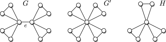
Figure 4: Example to show that $\mathcal{F}$-Edge-Removal is not minor-closed.

Appendix B Disconnected Planar-$\mathcal{F}$-Deletion has not finite integer index

We proceed to prove that if $\mathcal{F}$ is a family of graphs containing some disconnected graph $H$ (planar or non-planar), then the $\mathcal{F}$-Deletion problem has not finite integer index (FII) in general.

We shall use the equivalent definition of FII as suggested for graph optimization problems, see [23]. For a graph problem $o$-$\Pi$, the equivalence relation $\sim_{o\text{-}\Pi,t}$ on $t$-boundaried graphs is defined as follows. Let $G_{1}$ and $G_{2}$ be two $t$-boundaried graphs. We define $G_{1}\sim_{\Pi,t}G_{2}$ if and only if there exists an integer $i$ such that for any $t$-boundaried graph $H$, it holds $\pi(G_{1}\oplus H)=\pi(G_{2}\oplus H)+i$, where $\pi(G)$ denotes the optimal value of problem $o$-$\Pi$ on graph $G$. We claim that $G_{1}\sim_{\Pi,t}G_{2}$ if and only if $G_{1}\equiv_{\Pi,t}G_{2}$ (recall Definition 8 of canonical equivalence), where $\Pi$ is the parameterized version of $o$-$\Pi$ with the solution size as a parameter. Suppose $G_{1}\sim_{\Pi,t}G_{2}$ and let $\pi(G_{1}\oplus H)=\pi(G_{2}\oplus H)+i$. Then

$$(G_{1}\oplus H,k)\in\Pi\ \rightleftharpoons\ \pi(G_{1}\oplus H)\leqslant k\ \rightleftharpoons\ \pi(G_{2}\oplus H)\leqslant k-i(G_{2}\oplus H,k-i)\in\Pi,$$

and thus the forward implication holds. The opposite direction is easy to see.

Let $F_{1}$ and $F_{2}$ be two incomparable graphs with respect to the minor relation, and let $F$ be the disjoint union of $F_{1}$ and $F_{2}$. For instance, if we want $F$ to be planar, we can take $F_{1}=K_{4}$ and $F_{2}=K_{2,3}$. We set $\mathcal{F}=\{F\}$. Let $\Pi$ be the non-parameterized version of $\mathcal{F}$-Vertex Deletion.

For $i\geqslant 1$, let $G_{i}$ be the 1-boundaried graph consisting of the boundary vertex $v$ together with $i$ disjoint copies of $F_{1}$, and for each such copy, we add and edge between $v$ and an arbitrary vertex of $F_{1}$. Similarly, for $j\geqslant 1$, let $H_{j}$ be the 1-boundaried graph consisting of the boundary vertex $u$ together with $j$ disjoint copies of $F_{2}$, and for each such copy, we add and edge between $u$ and an arbitrary vertex of $F_{2}$.

By construction, if $i,j\geqslant 1$, it holds $\pi(G_{i}\oplus H_{j})=\min\{i,j\}$. Then, if we take $1\leqslant n<m$,

$$\pi(G_{n}\oplus H_{n-1})-\pi(G_{m}\oplus H_{n-1}) = (n-1)-(n-1)\ =\ 0,$$

$$\pi(G_{n}\oplus H_{m})-\pi(G_{m}\oplus H_{m}) = n-m\ <\ 0.$$

Therefore, $G_{n}$ and $G_{m}$ do not belong to the same equivalence class of $\sim_{\Pi,1}$ whenever $1\leqslant n<m$, so $\sim_{\Pi,1}$ has infinitely many equivalence classes, and thus $\Pi$ has not FII.

In particular, the above example shows that if $\mathcal{F}$ may contain some disconnected planar graph $H$, then Planar-$\mathcal{F}$-Deletion has not FII in general.

Appendix C MSO formula for topological minor containment

For a fixed graph $H$ we describe and MSO₁-formula $\Phi_{H}$ over the usual structure consisting of the universe $V(G)$ and a binary symmetric relation adj modeling $E(G)$ such that $G\models\Phi_{H}$ iff $H\preceq_{\mathit{tm}}\!G$.

$$\Phi_{H}(G) := \exists x_{v_{1}}\dots\exists x_{v_{r}}\exists D_{e_{1}}\dots\exists D_{e_{\ell}}$$

$$\Big{(}\,\enskip\bigwedge_{{\mathclap{1\leqslant i<j\leqslant r}}}x_{v_{i}}\neq x_{v_{j}}\wedge\bigwedge_{{\mathclap{\stackrel{{\scriptstyle 1\leqslant i\leqslant r}}{{1\leqslant j\leqslant\ell}}}}}x_{v_{i}}\not\in D_{e_{j}}\wedge\bigwedge_{\smash{\mathclap{1\leqslant i<j\leqslant r}}}\text{{\sc dis}}(D_{e_{i}},D_{e_{j}})\wedge\bigwedge_{\mathclap{\stackrel{{\scriptstyle 1\leqslant j\leqslant\ell}}{{e_{j}=v_{i}v_{k}}}}}\text{{\sc conn}}(x_{v_{i}},D_{e_{j}},x_{v_{k}})\,\Big{)}$$

$$\text{with}~{}\text{{\sc dis}}(X,Y) := \forall x(x\in X\rightarrow x\not\in Y)$$

$$\text{and}~{}\text{{\sc conn}}(u,X,v) := \exists w(\textsc{adj}(u,w)\wedge w\in X)\wedge\exists w(\textsc{adj}(v,w)\wedge w\in X)$$

$$\wedge\forall A\forall B((A\subseteq X\wedge B\subseteq X\wedge\text{{\sc dis}}(A,B))\rightarrow\exists a\exists b(a\in A\wedge b\in B\wedge\textsc{adj}(a,b)))$$

The subformula $\text{{\sc conn}}(u,X,v)$ expresses that $u,v$ are adjacent to $X$ and that $G[X]$ is connected, which implies that there exists a path from $u$ to $v$ in $G[X\cup\left\{u,v\right\}]$. By negation we can now express that $G$ does not contain $H$ as a topological minor, i.e. $G\models\neg\Phi_{H}$ iff $G$ is $H$-topological-minor-free.

References

- [1] K. A. Abrahamson and M. R. Fellows. Finite automata, bounded treewidth, and well-quasiordering. In Proc. of Graph Structure Theory, Contemporary Mathematics 147, pages 539–564. American Mathematical Society, 1991.
- [2] I. Adler, F. Dorn, F. V. Fomin, I. Sau, and D. M. Thilikos. Faster parameterized algorithms for minor containment. Theoretical Computer Science, 412(50):7018–7028, 2011.
- [3] J. Alber, M. R. Fellows, and R. Niedermeier. Polynomial-time data reduction for Dominating Set. Journal of the ACM, 51:363–384, 2004.
- [4] J. Battle, F. Harary, Y. Kadama, and J. Youngs. Additivity of the genus of a graph. Bulletin of the American Mathematical Society, 68:565–568, 1962.
- [5] H. L. Bodlaender. Dynamic programming on graphs with bounded treewidth. In Proc. of 15th ICALP, number 317 in LNCS, pages 105–118. Springer, 1988.
- [6] H. L. Bodlaender. A linear time algorithm for finding tree-decompositions of small treewidth. SIAM Journal on Computing, 25:1305–1317, 1996.
- [7] H. L. Bodlaender, F. V. Fomin, D. Lokshtanov, E. Penninkx, S. Saurabh, and D. M. Thilikos. (Meta) Kernelization. In Proc. of 50th FOCS, pages 629–638. IEEE Computer Society, 2009.
- [8] H. L. Bodlaender and E. Penninkx. A linear kernel for Planar Feedback Vertex Set. In Proc. of 3rd IWPEC, number 5018 in LNCS, pages 160–171. Springer, 2008.
- [9] H. L. Bodlaender, E. Penninkx, and R. B. Tan. A linear kernel for the -Disjoint Cycle problem on planar graphs. In Proc. of 19th ISAAC, number 5369 in LNCS, pages 306–317. Springer, 2008.
- [10] H. L. Bodlaender, S. Thomassé, and A. Yeo. Kernel bounds for disjoint cycles and disjoint paths. In Proc. of 17th ESA, number 5757 in LNCS, pages 635–646. Springer, 2009.
- [11] H. L. Bodlaender and B. van Antwerpen-de Fluiter. Reduction algorithms for graphs of small treewidth. Information and Computation, 167(2):86–119, 2001.
- [12] B. Bollobás and A. Thomason. Proof of a conjecture of Mader, Erdős and Hajnal on topological complete subgraphs. European Journal of Combinatorics, 19(8):883–887, 1998.
- [13] R. B. Borie, R. G. Parker, and C. A. Tovey. Automatic Generation of Linear-Time Algorithms from Predicate Calculus Descriptions of Problems on Recursively Constructed Graph Families. Algorithmica, 7(1):555–581, 1992.
- [14] J. R. Büchi. On a Decision Method in Restricted Second-Order Arithmetic. In Proc. of International Congress on Logic, Methodology, and Philosophy of Science, pages 1–11, 1962.
- [15] L. Cai. Fixed-parameter tractability of graph modification problems for hereditary properties. Information Processing Letters, 58:171–176, 1996.
- [16] J. Chen, H. Fernau, I. Kanj, and G. Xia. Parametric duality and kernelization: lower bounds and upper bounds on kernel size. SIAM Journal on Computing, 37:1077–1106, 2007.
- [17] J. Chen, F. V. Fomin, Y. Liu, S. Lu, and Y. Villanger. Improved algorithms for feedback vertex set problems. Journal of Computer and System Sciences, 74(7):1188–1198, 2008.
- [18] B. Courcelle. The Monadic Second-Order Theory of Graphs. I. Recognizable Sets of Finite graphs. Information and Computation, 85:12–75, 1990.
- [19] B. Courcelle and J. Engelfriet. Graph Structure and Monadic Second-Order Logic: A Language Theoretic Approach. Number 138 in Encyclopedia of Mathematics and its Applications. Cambridge University Press, June 2012.
- [20] M. Cygan, J. Nederlof, M. Pilipczuk, M. Pilipczuk, J. M. M. van Rooij, and J. O. Wojtaszczyk. Solving connectivity problems parameterized by treewidth in single exponential time. In Proc. of 52nd FOCS, pages 150–159. IEEE Computer Society, 2011.
- [21] M. Cygan, M. Pilipczuk, M. Pilipczuk, and J. Wojtaszczyk. An improved FPT algorithm and quadratic kernel for pathwidth one vertex deletion. In Proc. of 5th IWPEC, number 6478 in LNCS, pages 95–106. Springer, 2010.
- [22] A. Dawar, M. Grohe, and S. Kreutzer. Locally excluding a minor. In Proc. of 22 LICS, pages 270–279. IEEE Computer Society, 2007.
- [23] B. de Fluiter. Algorithms for Graphs of Small Treewidth. PhD thesis, Utrecht University, 1997.
- [24] F. K. H. A. Dehne, M. R. Fellows, M. A. Langston, F. A. Rosamond, and K. Stevens. An FPT algorithm for the undirected feedback vertex set problem. In Proc. of 11th COCOON, number 3595 in LNCS, pages 859–869. Springer, 2005.
- [25] R. Diestel. Graph Theory. Springer-Verlag, Heidelberg, 4th edition, 2010.
- [26] M. J. Dinneen. Too many minor order obstructions. Journal of Universal Computer Science, 3(11):1199–1206, 1997.
- [27] M. Dom, D. Lokshtanov, and S. Saurabh. Incompressibility through colors and IDs. In Proc. of 36th ICALP, number 5555 in LNCS, pages 378–389. Springer, 2009.
- [28] F. Dorn, F. V. Fomin, and D. M. Thilikos. Catalan structures and dynamic programming in -minor-free graphs. In Proc. of 19th SODA, pages 631–640. SIAM, 2008.
- [29] R. G. Downey and M. R. Fellows. Parameterized Complexity. Springer-Verlag, 1999.
- [30] M. R. Fellows and M. A. Langston. Nonconstructive tools for proving polynomial-time decidability. Journal of the ACM, 35:727–739, 1988.
- [31] J. Flum and M. Grohe. Parameterized Complexity Theory. Springer-Verlag, 2006.
- [32] F. V. Fomin, B. M. P. Jansen, and M. Pilipczuk. Preprocessing Subgraph and Minor Problems: When Does a Small Vertex Cover Help? CoRR, abs/1206.4912, 2012.
- [33] F. V. Fomin, D. Lokshtanov, N. Misra, G. Philip, and S. Saurabh. Hitting forbidden minors: Approximation and kernelization. In Proc. of 28th STACS, volume 9 of LIPIcs, pages 189–200. Schloss Dagstuhl–Leibniz-Zentrum für Informatik, 2011.
- [34] F. V. Fomin, D. Lokshtanov, N. Misra, and S. Saurabh. Nearly optimal FPT algorithms for Planar--Deletion. Unpublished manuscript, 2011.
- [35] F. V. Fomin, D. Lokshtanov, N. Misra, and S. Saurabh. Planar -Deletion: Approximation and Optimal FPT Algorithms. To appear in Proc. of 53rd FOCS. Available at CoRR, abs/1204.4230, 2012.
- [36] F. V. Fomin, D. Lokshtanov, N. Misra, and S. Saurabh. Planar- Deletion: Kernelization and obstruction bounds. Unpublished manuscript, 2012.
- [37] F. V. Fomin, D. Lokshtanov, S. Saurabh, and D. M. Thilikos. Bidimensionality and kernels. In Proc. of 21st SODA, pages 503–510. SIAM, 2010.
- [38] F. V. Fomin, D. Lokshtanov, S. Saurabh, and D. M. Thilikos. Linear kernels for (Connected) Dominating Set on -minor-free graphs. In Proc. of 23rd SODA, pages 82–93. SIAM, 2012.
- [39] F. V. Fomin, S. Oum, and D. M. Thilikos. Rank-width and tree-width of -minor-free graphs. European Journal of Combinatorics, 31(7):1617–1628, 2010.
- [40] M. Frick and M. Grohe. The complexity of first-order and monadic second-order logic revisited. Annals of Pure and Applied Logic, 130(1–3):3–31, 2004.
- [41] M. Grohe and D. Marx. Structure theorem and isomorphism test for graphs with excluded topological subgraphs. CoRR, abs/1111.1109, 2011.
- [42] J. Guo, J. Gramm, F. Hüffner, R. Niedermeier, and S. Wernicke. Compression-based fixed-parameter algorithms for feedback vertex set and edge bipartization. Journal of Computing and System Sciences, 72(8):1386–1396, 2006.
- [43] J. Guo and R. Niedermeier. Linear problem kernels for NP-hard problems on planar graphs. In Proc. of 34th ICALP, number 4596 in LNCS, pages 375–386. Springer, 2007.
- [44] J. Guo, R. Niedermeier, and S. Wernicke. Fixed-parameter tractability results for full-degree spanning tree and its dual. Networks, 56(2):116–130, 2010.
- [45] G. Joret, C. Paul, I. Sau, S. Saurabh, and S. Thomassé. Hitting and harvesting pumpkins. In Proc. of 19th ESA, number 6942 in LNCS, pages 394–407. Springer, 2011.
- [46] I. A. Kanj, M. J. Pelsmajer, M. Schaefer, and G. Xia. On the Induced Matching problem. Journal of Computer and System Sciences, 77(6):1058–1070, 2011.
- [47] K. Kawarabayashi. Planarity allowing few error vertices in linear time. In Proc. of 50th FOCS, pages 639–648. IEEE Computer Society, 2009.
- [48] E. J. Kim, C. Paul, and G. Philip. A single-exponential FPT-algorithm for -minor cover problem. In Proc. of 13th SWAT, number 7357 in LNCS. Springer, 2012. To appear.
- [49] T. Kloks. Treewidth, Computations and Approximations. Number 842 in LNCS. Springer, 1994.
- [50] J. Komlós and E. Szemerédi. Topological cliques in graphs II. Combinatorics, Probability and Computing, 5(01):79–90, 1996.
- [51] S. Kreutzer. Algorithmic meta-theorems. Electronic Colloquium on Computational Complexity, 16:147, 2009.
- [52] S. Kreutzer and S. Tazari. On brambles, grid-like minors, and parameterized intractability of monadic second-order logic. In Proc. of 21st SODA, pages 354–364. SIAM, 2010.
- [53] J. M. Lewis and M. Yannakakis. The node-deletion problem for hereditary properties is NP-complete. Journal of Computer and System Sciences, 20(2):219–230, 1980.
- [54] D. Lokshtanov. Wheel-free deletion is -hard. In Proc. of 3rd IWPEC, number 5018 in LNCS, pages 141–147. Springer, 2008.
- [55] D. Lokshtanov, D. Marx, and S. Saurabh. Slightly superexponential parameterized problems. In Proc. of 22nd SODA, pages 760–776. SIAM, 2011.
- [56] D. Lokshtanov, M. Mnich, and S. Saurabh. A linear kernel for Planar Connected Dominating Set. Theoretical Computer Science, 412(23):2536–2543, 2011.
- [57] D. Lokshtanov, S. Saurabh, and S. Sikdar. Simpler parameterized algorithm for OCT. In Proc. of 20th IWOCA, number 5874 in LNCS, pages 380–384. Springer, 2009.
- [58] D. Marx. Chordal Deletion is fixed-parameter tractable. Algorithmica, 57(4):747–768, 2010.
- [59] D. Marx and I. Schlotter. Obtaining a planar graph by vertex deletion. Algorithmica, 62(3–4):807–822, 2012.
- [60] B. Mohar. An obstruction to embedding graphs on surfaces. Discrete Mathematics, 78(1–2):135–142, 1989.
- [61] H. Moser and S. Sikdar. The parameterized complexity of the Induced Matching problem. Discrete Applied Mathematics, 157(4):715–727, 2009.
- [62] Anil Nerode. Linear Automaton Transformations. Proceedings of the American Mathematical Society, 9:541–544, 1958.
- [63] J. Nešetřil and P. Ossona de Mendez. On nowhere dense graphs. European Journal of Combinatorics, 32(4):600–617, 2011.
- [64] R. Niedermeier. Invitation to Fixed-Parameter Algorithms. Oxford University Press, 2006.
- [65] G. Philip, V. Raman, and Y. Villanger. A quartic kernel for Pathwidth-One Vertex Deletion. In Proc. of 36th WG, number 6410 in LNCS, pages 196–207. Springer, 2010.
- [66] B. A. Reed, K. Smith, and A. Vetta. Finding odd cycle transversals. Operations Research Letters, 32(4):299–301, 2004.
- [67] N. Robertson and P. D. Seymour. Graph minors II. Algorithmic aspects of tree-width. Journal of Algorithms, 7:309–322, 1986.
- [68] N. Robertson and P. D. Seymour. Graph minors V. Excluding a planar graph. Journal of Combinatorial Theory, Series B, 41:92–114, 1986.
- [69] N. Robertson and P. D. Seymour. Graph minors X. Obstructions to tree-decomposition. Journal of Combinatorial Theory, Series B, 52:153–190, 1991.
- [70] N. Robertson and P. D. Seymour. Graph minors XIII. The disjoint paths problem. Journal of Combinatorial Theory, Series B, 63:65–110, 1995.
- [71] J. Rué, I. Sau, and D. M. Thilikos. Dynamic programming for graphs on surfaces. CoRR, abs/1104.2486, 2011. To appear in ACM Transactions on Algorithms.
- [72] A. Thomason. The extremal function for complete minors. Journal of Combinatorial Theory, Series B, 81(2):318–338, 2001.
- [73] M. Yannakakis and F. Gavril. Edge dominating sets in graphs. SIAM Journal of Applied Mathematics, 38(3):364–372, 1980.